Universidade do Minho
Escola de Engenharia
Cristiano Rafael da Silva Sousa
Efficient sequential and parallel versions of
MST-solvers for multi-core CPU-chips and
GPUs
Universidade do Minho
Dissertação de Mestrado
Escola de Engenharia
Departamento de Informática
Cristiano Rafael da Silva Sousa
Efficient sequential and parallel versions of
MST-solvers for multi-core CPU-chips and
GPUs
Mestrado em Engenharia Informática
Trabalho realizado sob orientação de
Alberto José Proença
Acknowledgements
Ao meu orientador, Alberto Proença, que desde o meu primeiro ano da Licenciatura sempre me inspirou pelo seu rigor e brio académico, e pela orientação, tanto durante a dissertação como a nível pessoal. Ao meu coorientador, Artur Mariano, pela oportunidade desta dissertação, pelo seu acompanhamento, e por durante este ano ter sido muito mais para mim do que um coorientador, deixo um grande obrigado.
Aos Professores que mais me marcaram durante o meu percurso na Universidade do Minho: Alberto José Proença, José Nuno Oliveira, Jorge Sousa Pinto, Luís Paulo Santos, Manuel Alcino Cunha, António Luís Sousa, António Ramires Fernandes, Rui Mendes, Maria João Frade, Luís Silva Dias e Ana Cordeiro.
I would also like to thank Rupesh Nasre, who was my advisor during my internship at the University of Texas at Austin, for his excellent guidance during the internship, for the availability and willingness to help even after the internship, and for helping me shape the next few years of my professional life.
À Família que criei nestes cinco anos na Universidade deixo um abraço sentido. Os nomes são em demasia para serem enumerados, mas eles sabem quem são, e sabem que guardam todos um lugar especial no meu coração. Tudo que eu hoje sou, devo a eles.
Quero também deixar um agradecimento especial à Catarina Azevedo, que me apoiou e acompanhou de perto durantes estes últimos meses difíceis. Sem ela, esta dissertação não teria sido possível.
Acima de tudo, quero agradecer aos meus pais, irmã e irmão, que, apesar de estarem muito longe de mim, sempre me apoiaram e motivaram, e a quem eu sempre quis fazer orgulhosos. Para o meu pequeno irmão espero ter sido uma inspiração.
Agradeço a todos os meus amigos e familiares pela compreensão dada à minha ausência durante este ano. Dedico esta tese aos meus Irmãos e familiares que partiram deste mundo.
Em memória do meu tio e padrinho
In memory of my uncle and godfather
José António Oliveira de Sousa
05/12/1963 - 03/07/2013
...
Em memória da minha avó
In memory of my grandmother
Olívia de Brito Mota
27/06/1936 - 22/01/2015
...
Em memória do meu tio
In memory of my uncle
Joaquim Pinto Penha Cerqueira
04/08/1959 - 06/10/2014
...
E, em memória dos meus Irmãos
And, in memory of my Brothers
João Pedro Gonçalves Rei de Abreu Vieira
17/10/1995 - 23/04/2014
Vasco Alexandre Ferreira Rodrigues
12/03/1995 - 23/04/2014
Nuno Miguel de Araújo Caldeira Ramalho
Abstract
The Minimum Spanning Tree (MST) problem is a well known graph problem that plays an important role in various scientific fields. Graph algorithms are known to be irregular, namely due to the unpredictable memory access patterns and workload distribution among the graph vertices. These problems place ad-ditional challenges on novel parallel computing systems, namely those that resort to a mix of shared and distributed memory paradigms and to heterogeneous computing environment with attached computing ac-celerators, such as many-core CPU-chips and GPU devices. This dissertation addresses these challenges, as to develop efficient implementations of MST-solvers.
Sequential implementations of the three key MST algorithms - Borůvka’s, Kruskal’s and Prim’s algo-rithm - have been implemented, tested and compared in terms of performance. Parallel implementations of Prim’s and Borůvka’s algorithms were also implemented and tested using the same suite of widely used road-network graphs. This comparative analysis included a first-hand comprehensive empirical comparison of several disclosed state of the art third-party CPU and GPU implementations of MST-solvers.
A parallel algorithmic variant of Borůvka’s algorithm was devised, which exhibited speedups that out-performed all other tested competitors. The functionality of this variant is shown to be easily ported to other shared and distributed memory systems, including heterogeneous systems with GPU devices, without plac-ing constraints on the graph size or hurtplac-ing performance.
Resumo
Versões sequenciais e paralelas eficientes de algoritmos de
árvores de extensão mínima para CPUs e GPUs
O problema da árvore de extensão mínima (MST) é um problema de grafos muito conhecido e tem um papel importante em várias áreas científicas. Os algoritmos de grafos são conhecidos por serem irregulares, nomeadamente devido aos padrões de acesso à memória imprevisíveis, e à distribuição de trabalho pelos vértices do grafo. Estes problemas impoem um maior desafio nas novas plataformas de computação paralela, em particular aquelas que recorrem à mistura de memoria partilhada e distribuída, e a ambientes heterogéneos com aceleradores, como os many-core CPUs e dispositivos GPU. Esta dissertação aborda estes desafios, a fim de desenvolver implementações eficientes de MST-solvers.
Os três principais algoritmos de MST - Borůvka, Kruskal e Prim- foram implementados em sequencial, testadas e comparadas em termos de performance. Implementações paralelas dos algoritmos de Prim e Borůvka também foram implementadas e testadas usando o mesmo conjunto de grafos de estradas rodoviárias. Esta análise comparativa inclui uma comparação empírica de primeira-mão de vários
MST-solversde terceiros.
Foi desenvolvida uma variante algorítmica paralela do algoritmo de Borůvka, que mostrou ganhos de desempenho que superam a concorrência. É mostrado que a funcionalidade desta variante é facilmente portada, sem restringir o tamanho dos grafos ou prejudicar o desempenho, para outros sistemas de me-mória partilhada e distribuída, aonde se incluem sistemas heterogéneos com dispositivos GPU.
Contents
Contents xi
List of Figures xv
List of Tables xvii
List of Algorithms xix
1 Introduction 1
1.1 The Minimum Spanning Tree problem . . . 1
1.2 Challenges and Motivation . . . 2
1.3 Goals and Contributions . . . 3
1.4 Dissertation Structure . . . 3
2 Heterogeneous Computing Platforms 5 2.1 Multi-core architectures . . . 6
2.1.1 Libraries . . . 7
2.2 Many-core architectures . . . 9
2.2.1 Graphic Processing Units (GPUs) . . . 9
3 Minimum Spanning Tree Solvers 13 3.1 Sequential Minimum Spanning Tree Algorithms . . . 13
3.1.1 Borůvka’s Algorithm . . . 14
3.1.2 Kruskal’s Algorithm . . . 16
3.1.3 Prim’s Algorithm . . . 18
3.2 State of the Art of Sequential and Parallel Implementations . . . 21
3.2.1 SMP Systems and Multi-Core CPU-Chips . . . 21
CONTENTS
3.2.3 GPUs . . . 22
3.2.4 Conclusions . . . 24
4 Parallel Algorithms and Implementations 25 4.1 Graph representation . . . 25
4.2 Lock-Free Adjacency List . . . 27
4.3 Multiple Instance Prim . . . 28
4.3.1 Collision Treatment . . . 29
4.3.2 Partitioned . . . 31
4.3.3 Conclusions . . . 34
4.4 A Generic Borůvka’s Algorithm . . . 35
4.4.1 Algorithm . . . 35 4.4.2 Implementation Details . . . 39 5 Performance Evaluation 41 5.1 Experimental Environment . . . 41 5.2 Data sets . . . 42 5.2.1 Real-life graphs . . . 43 5.2.2 Synthetic graphs . . . 43
5.3 Description of the Implementations . . . 44
5.3.1 Dissertation Implementations . . . 44
5.3.2 Third-Party Implementations . . . 45
5.4 Experimental Results . . . 45
5.5 Critical Analysis . . . 53
6 Conclusions & Future Work 57 6.1 Conclusions . . . 57
6.2 Future Work . . . 58
Bibliography 59
A Generic Borůvka’s Algorithm Pseudo-Code 63
Acronyms
API Application Programming Interface BGL Boost Graph Library
CPU Central Processing Unit CSR Compressed Sparse Row
CUDA Compute Unified Device Architecture CUDPP CUDA Data Parallel Primitives Library EREW Exclusive Read Exclusive Write
FLOPS/s Floating Point Operations per Second FPGA Field-programmable gate array
FSB Front-Side Bus
GPGPU General Purpose Graphics Processing Unit GPU Graphics Processing Unit
HPC High Performance Computing HT HyperTransport
ACRONYMS
MIC Many Integrated Core MPI Message Passing Interface MST Minimum Spanning Tree NUMA Non-Uniform Memory Access OpenCL Open Computing Language
PAPI Performance Application Programming Interface PCIe PCI express
PRAM Parallel Random Access Machine QPI QuickPath Interconnect
R-MAT Recursive Matrix
SIMD Single Instruction Multiple Data SIMT Single Instruction Multiple Thread SM Streaming Multiprocessor
SMP Symmetric multiprocessing SPMD Single Program Multiple Data STM Software Transactional Memory TBB Threading Building Blocks UMA Uniform Memory Access VLSI Very-Large-Scale Integration
List of Figures
1.1 Example graph. . . 1
2.1 Multi-core architectures. . . 6
2.2 Distributed memory system.. . . 7
2.3 Representation of NVIDIA GK110 Kepler (courtesy of NVIDIA) . . . 11
3.1 Borůvka’s algorithm. . . 15
3.2 Kruskal’s algorithm. . . 17
3.3 Prim’s algorithm. . . 19
4.1 Representations of the example graph in Figure 1.1. . . 26
4.2 Example of multi instanced Prim . . . 29
4.3 Simple example of an incorrectly added edge. . . 31
4.4 Complex example of an incorrectly added edge. . . 33
4.5 Cycle creation with 3 partitions. . . 33
4.6 Find minimum edge per vertex. . . 36
4.7 Remove mirrored edges. . . 36
4.8 Initiaize and propagate colors. . . 37
4.9 Create new vertex ids.. . . 37
4.10 Count, assign, and insert new edges. . . 38
5.1 Measured execution times of the sequential implementations for all road-network graphs. 46 5.2 Scalability for USA road-network graph. . . 46
5.3 Execution time breakdown forprim_union.. . . 47
5.4 (%) vertices processed per thread bytm_mst_ptfor execution with 2 threads on USA graph. 48 5.5 Average load imbalance per iteration forGenBoruvka OMPfor the USA road-network graph. 50 5.6 L3 cache miss rate per iteration forGenBoruvka OMPfor USA road-network graph. . . . 52
LIST OF FIGURES
5.8 Measured execution times for all road-network graphs . . . 54
5.9 Measurements for NE road-network graph.. . . 55
5.10 Measurements for PT road-network graph. . . 56
List of Tables
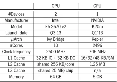
5.1 System characteristics. . . 42
5.2 Road-network graphs used in benchmarks. . . 43
5.3 Speedup (S) and Efficiency (E) forGenBoruvka OMPandGenBoruvka GPUfor 3 graphs with respect toGenBoruvka OMPimplementation with a single thread. . . 49
List of Algorithms
1 Borůvka’s algorithm . . . 16
2 Kruskal’s algorithm . . . 17
3 Prim’s algorithm . . . 20
4 Prim’s algorithm using a priority queue . . . 20
5 Parallel Borůvka variant . . . 35
6 Parallel, distributed memory, Borůvka variant . . . 40
7 Find minimum edge per vertex . . . 63
8 Remove mirrored edges kernel . . . 64
9 Initialize colors . . . 64
10 Propagate colors kernel . . . 64
11 Create new vertex ids . . . 64
12 Count new edges . . . 65
Chapter 1
Introduction
1.1 The Minimum Spanning Tree problem
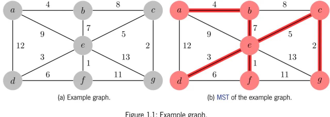
Given a connected, undirected, weighted graph G(V, E), where V is the set of vertices and E the set of edges, theMinimum Spanning Tree (MST)of G is the sub-graph T that spans all vertices of G and has
|V | − 1 edges, such that no cycles are formed and the total weight is minimized. If all edge weights are
distinct then the graph’sMSTis unique, otherwise severalMSTsare possible. An example graph and its correspondingMSTis shown in Figure1.1.
TheMSTproblem is a well known graph problem and plays an important role in various scientific fields, such as in theVery-Large-Scale Integration (VLSI)circuit layout, in road, electrical and computer networks and in the approximation of the traveling salesman problem. Since 1926, when it was seen firsthand, the
. . a . b . c . d . e . f . g . 4 . 8 .12 . 9 . 7 . 5 . 3 . 6 . 1 . 2 . 13 . 11
(a) Example graph.
. . a . b . c . d . e . f . g . 4 . 8 .12 . 9 . 7 . 5 . 3 . 6 . 1 . 2 . 13 . 11 . a . b . e . f . d . c . g
(b)MSTof the example graph.
CHAPTER 1. INTRODUCTION
MST problem had undergone an extensive study on both sequential and parallel implementations.
This class of algorithms is known as irregular, i.e., both the workload and memory access patterns cannot be predicted at compile time, as they depend on the graph structure. Efforts are nowadays reserved to map these irregular algorithms onto parallel computing platforms.
1.2 Challenges and Motivation
Algorithms with regular memory accesses, such as matrix multiplication and linear system solvers, have undergone extensive studies. Highly efficient implementations have been developed, for various computing platforms and for a wide variety of these algorithms. This class of algorithms no longer poses a real challenge for researches.
Graphs are increasingly being used to represent social-, road- and computer-networks, but also in the medical field with genome sequencing and electroencephalographies. Algorithms that process graphs are much more complex and challenging to parallelize due to their inherent irregularity. As such, graph algo-rithms are becoming an attractive option not only to solve real-life problems, but also to benchmark the quality, performance, and productivity of the development frameworks to deploy, efficiently, portability of applications across distinct heterogeneous computing platforms.
With the advent of new computing platforms - such asGraphic Processing Units (GPUs)- and program-ming paradigms - such as shared and distributed memory - the algorithms no longer are the sole focus of research, when trying to extract performance from their implementations. Each paradigm has their own characteristics, and programmers are forced to understand the underlying architecture and technical details, if they are to develop efficient implementations.
Aside from figuring out ways to parallelize the algorithm, the partitioning of the workload and associated data must be taken into consideration. How are the parallel tasks and associated data distributed among the threads, processes and computing devices? How does one leverage this with inter-task communications, data locality in shared memory systems, and the data transfer overhead in distributed memory systems? When the application is efficiently deployed for one platform, is the same algorithm, and corresponding par-allel code, efficiently distributed among the available computing resources, on other computing platforms, without further tuning? These are some of the challenges that are nowadays reserved for parallelizing algorithms.
1.3. GOALS AND CONTRIBUTIONS
1.3 Goals and Contributions
This dissertation aims to research and extend the state of the art ofMST-solvers, while also assessing both sequential and parallel versions ofMST-solvers, for multi-coreCentral Processing Unit (CPU)-chips and
GPUs. The goal is to better understand MST-solver suitability to parallel architectures, and find ways to improve it. In particular, efficient parallel version for bothCPUsandGPUs, should be implemented. As a final goal of this dissertation work, a new parallel version of anMST-solver is expected to be devised.
Throughout this dissertation, various existing and novel MST-solver algorithms are devised and imple-mented, from which a generic Borůvka’s algorithm stands out for its portability across computing devices and high performance. A compilation of the existing state of the art ofMST-solvers, and a comprehensive comparison with these solvers and the solvers developed in the context of this dissertation, are included.
The work on the generic Borůvka’s algorithm resulted in a scientific paper that was submitted and accepted at an top tier conference: the 23rd Parallel, Distributed and Network-based Processing (PDP 2015). The accepted paper can be found in AppendixB.
1.4 Dissertation Structure
The rest of this dissertation is presented with the following chapter structure:
Ch.
2
Heterogeneous Computing Platforms
This chapter overviews the state of the art of computing platforms, focusing on multi-coreCPU-chips in both shared and distributed memory programming models and on many-core devices, with a special emphasis onGPUdevices. It also presents some relevant libraries used on these programming platforms, namely those used in the context of this dissertation.
CHAPTER 1. INTRODUCTION
Ch.
3
Minimum Spanning Tree Solvers
This chapter introduces the key algorithms and implementations that have been developed so far to compute the MST. It presents and details three seminal MST-solvers: Borůvka’s, Kruskal’s and Prim’s algorithms. The last section overviews the literature on existing sequential and parallel implementations.
Ch.
4
Parallel Algorithms and Implementations
This chapter presents the new parallel MST-solver implementations developed in the context of this dissertation, and introduces the data structures used to represent graphs, and which are used for represen-tation in the parallel implemenrepresen-tations. It also presents parallelization and implemenrepresen-tations details of the multiple instance Prim’s algorithm, as described in Chapter 3, addressing collision resolution strategies, and partitioning approaches. Lastly, a parallel, platform-independent, algorithmic variant of Borůvka’s algorithm is presented, addressing the key issues to a platform independent variant.
Ch.
5
Performance Evaluation
This chapter describes the experimental environment, including a detailed description of the computing platforms, external libraries used and graphs that were used for testing purposes. It presents the exper-imental study conducted in the context of this dissertation, including a comparative analysis of all the implementations that were developed in the context of this dissertation, and a critical analysis between the best implementation developed in this dissertation, with third-party MST-solvers
Ch.
6
Conclusions & Future Work
This chapter concludes the dissertation, presenting an overview of the results obtained with the devel-oped implementations and suggesting lines of research to further investigate the more relevant outcome of this work.
Chapter 2
Heterogeneous Computing Platforms
This chapter overviews the state of the art of computing platforms, focusing on multi-core
CPU-chips in both shared and distributed memory programming models and on many-core devices, with a special emphasis onGPU devices. It also presents some relevant libraries used on these programming platforms, namely those used in the context of this dissertation.
With scientific problems of the most diverse areas expanding their research, more people are resorting to computer applications to solve their problems. However, the time needed to solve these problems put a strain on the size of the data and the complexity of the application. To meet the consumers’ demand,CPU
chips became faster and more complex. However, the ever growing search for more computing power even-tually faced power consumption and heat dissipation problems. The strategy adopted by major hardware companies was to simplify the cores, and pack multiple cores on a single chip. Previously, programmers did not need to worry with parallelism. Existing implicit parallelism such as pipeline supersclarity and out-of-order execution is handled by the compiler and the chip hardware, and multi-threaded execution involved only the parallel execution of different processes. To take advantage of the multi-core processor devices, a new programming model surfaced that allows explicit parallel code to be written within the application.
Algorithms that exhibited regular memory access patterns became a popular target for vectorization (Single Instruction Multiple Data (SIMD)), allowing the same instruction to be applied to a set of data. To address the growing amount of data, devices that target massive data parallelism were developed. The general term associated to these devices isaccelerators.
CHAPTER 2. HETEROGENEOUS COMPUTING PLATFORMS
The termheterogeneous computing platformhas been thrown around frequently with different meanings. In this dissertation we will assume that a heterogeneous computing platform is a single computing node with one or more multi-coreCPU-chips with attached accelerator devices. In turn, multiple heterogeneous nodes can be interconnected to form a computer cluster.
2.1 Multi-core architectures
Up until recently, most of the focus on parallel algorithms has been targeted to multi-coreCPU-chips. The shared memory model, where different threads share the same memory space, has been the primary target for parallel implementations. In the shared memory model, theUniform Memory Access (UMA)and
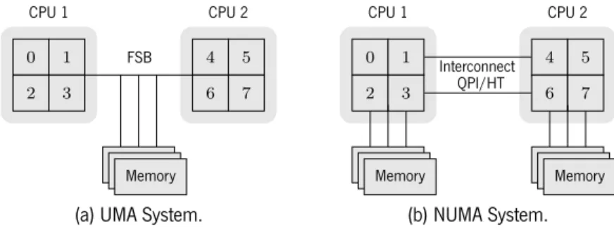
Non-Uniform Memory Access (NUMA)memory paradigms can be distinguished.UMAis more common, all threads have an uniform access time to the memory banks, whileNUMArefers to a memory layout where memory access latency depends on the location of the running thread and the memory region it is trying to access. TheNUMAparadigm is currently present in single computing nodes with more than oneCPU-chip, and the non-uniform latency is due to the fact that currentCPU-chips include on-chip the memory controllers. As a result, different memory banks are connected to distinctCPUs. Cross memory bank access is possible due to proprietary interconnects between theCPU-chips, such as the IntelQuickPath Interconnect (QPI)or AMDHyperTransport (HT). This interconnect replaces theFront-Side Bus (FSB)used inUMAsystems. Time is being spent to figure out ways to take advantage of these systems, and how thread and memory affinity affects the application performance. However, performance scalability is limited to the number of cores and
CPUs a single computing node can harbor. Figure2.1illustrates the difference betweenUMA andNUMA
systems. . . 0 . 1 . 2 . 3 . 4 . 5 . 6 . 7 . Memory . Memory . Memory . CPU 1 . CPU 2 . FSB
(a) UMA System.
. . 0 . 1 . 2 . 3 . 4 . 5 . 6 . 7 . Memory . Memory . Memory . Memory . Memory . Memory . CPU 1 . CPU 2 . Interconnect . QPI/HT (b) NUMA System.
Figure 2.1: Multi-core architectures.
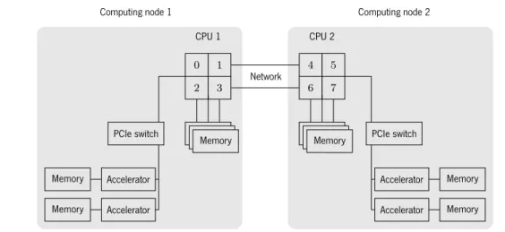
In the distributed memory model, each process works in their own private memory space. The private memory spaces is due to either the programming model employed, or by being physically separated, which is
2.1. MULTI-CORE ARCHITECTURES . . 0 . 1 . 2 . 3 . 4 . 5 . 6 . 7 . Memory . Memory . Memory . Memory . Memory . Memory . CPU 1 . CPU 2 . Computing node 1 . Computing node 2 . Network . PCIe switch . Accelerator . Memory . Accelerator . Memory . PCIe switch . Accelerator . Memory . Accelerator . Memory
Figure 2.2: Distributed memory system.
the case when working with accelerators or in a multi-node environment. Note that each of these computing nodes are heterogeneous platforms, i.e., they can have multiple CPUs with attached accelerators. The sharing of data is achieved by inter-process communication, which has an added overhead. Scalability is limited to the the amount of communication. Figure2.2shows a distributed system with twoUMAcomputing nodes, each with two accelerators. The interfaces that connects theCPUwith its memory, the accelerator with its memory,PCI express (PCIe), which connects the CPUto the accelerator, and the network, which interconnects the computing nodes, all operate at different transfer rates. The various memory regions are not shared, which can create bottlenecks if communication is not dealt with properly.
2.1.1 Libraries
In the context of multi-core architectures, several libraries have been developed to aid the development of efficient parallel applications. The libraries used in this dissertation are overviewed below.
OpenMP
OpenMP is a high levelApplication Programming Interface (API)for developing parallel application on shared memory systems, offering a simple way to parallelize applications, using compiler directives for work sharing constructs, synchronization and reduction to a single variable. Furthermore, various schedulers are available to assign loop iterations to each thread.
CHAPTER 2. HETEROGENEOUS COMPUTING PLATFORMS
IntelThreading Building Blocks(TBB)
IntelThreading Building Blocks (TBB)is a task based, C++ template library and is somewhat similar to OpenMP, in the sense that it offers various work sharing constructs such as for, reduce, and scan. However,
TBBis more low level, in comparison to OpenMP, as parallelization is achieved using template classes, and offering concurrent containers, pipelines, parallel sort and mutexes. Scheduling is done at a task level, which are dynamically allocated to each core, and work stealing is used to ensure efficient use of the available resources.
pThreads
When more control is need in the development of parallel applications, one must resort to a more low level library. pThreads is the POSIX standard for threads, and offers full control on the creation and joining of threads. Furthermore, it also implements low level synchronization primitives such as mutexes, condition variables and barriers, leaving the responsibility of thread management entirely to the user. When using pThreads, complications, such as deadlocks, may arise. However, it also offers much more control, which is often necessary to parallelize complex algorithms.
OpenMPI
OpenMPI is an open sourceMessage Passing Interface (MPI)library for developing distributed memory applications and offers anAPIwith a wide range of optimized primitives, such as barriers, broadcast, gather, scatter, scan and reduce, all of which implement various variants, such as synchronous, asynchronous and variable length message sizes. OpenMPI works over ethernet protocols, but also over proprietary interconnect networks such as Myrinet and Infiniband, while transparently working over shared memory when the processes are running on the same computing node.
Together with OpenMP, this can be used to develop hybrid applications to run on clusters, using OpenMPI to parallelize the application among computing nodes, and, in turn, OpenMP to parallelize each process, effectively obtaining a hybrid shared and distributed memory application.
2.2. MANY-CORE ARCHITECTURES
Performance Application Programming Interface(PAPI)
ThePerformance Application Programming Interface (PAPI)is a portable interface that allows the user to access and collect low level performance counters. The available counters depends on the underlying
CPU. UsingPAPI, an application’s miss rates for all cache levels, load balance, floating point operations per second, operational intensity, estimate bandwidth used, and many other metrics can be measured. This allows one to identify and address bottlenecks, and make grounded assertions on the limited performance of applications.
2.2 Many-core architectures
The many-core architecture devices, oraccelerators, was the industry response to massive data parallel algorithms. These accelerators are off-chip devices with tens to thousands of cores and their own memory space. Active memory transfer between the main memory and the accelerator’s memory is possible. However, the latency is high and transfer times may have a significant impact on performance, so these must be taken into account when building efficient applications for these devices. Furthermore, the private memory space is rather small compared to the main memory, limiting the possible input size and forcing frequent memory transfers. Often programmers stray away from accelerators, namely when their algorithms do not map well onto them and performance lacks due to memory transfers, completely overtaking execution time.
Several devices are currently available and popular, the most notable being theGeneral Purpose Graphics Processing Unit (GPGPU), the Field-programmable gate array (FPGA) and the IntelMany Integrated Core (MIC)family, currently represented by the Xeon Phi.
2.2.1
Graphic Processing Units
(
GPUs
)
Previously,GPUswere devices dedicated to processing and creating images to be shown on a graphics display. Since 2006, theGPU is becoming a more general computing device, targeted to massive data parallelism. These newGPGPUshave hundreds, to thousands of very simple cores. The new programming model employed forced programmers to adapt their algorithms and understand the underlying architecture.
CHAPTER 2. HETEROGENEOUS COMPUTING PLATFORMS
Two well known frameworks for programming on theGPUsis theOpen Computing Language (OpenCL)
and NVIDIA’s Compute Unified Device Architecture (CUDA), the largest open and proprietary frameworks, respectively. In this dissertation, the latter is used.
At the hardware level, the GPUis composed by severalStreaming Multiprocessors (SMs)(changed in to SMX with the Kepler architecture), which, in turn, are composed by several execution units, known as
CUDA cores. In the Kepler architecture, each SMX has 192 CUDAcores, each basically containing one single precision floating point execution unit, and an integer execution unit. Furthermore, the SMXs also contain additional functional units: double precision floating point units and load/store units
ACUDAkernel is a piece of code that every thread is going to execute, as a parallel task, on theGPU. The threads are grouped into blocks of user-specified size. The collection of all blocks of a kernel is called a grid Each block is assigned to anSMand broken down into warps of 32 threads for execution. All threads inside the same warp execute the same instruction at a given time. From this, it is clear that the CUDA
model uses both theSIMDandSingle Instruction Multiple Thread (SIMT)models at warp level, andSingle Program Multiple Data (SPMD)at kernel level. The number of blocks, threads and warps that can reside in eachSMis limited and depends on the specific architecture.
Each thread has access to a set of registers that is managed by the hardware, and an L1 and L2 cache with 64 KB and 1.5 MB, respectively, for the Kepler architecture. All threads in the same block also have access to a fast shared memory region that is managed by the user. The total size available for L1 cache and shared memory is distributed among them, but can be configured by the user in predefined combination of sizes. Lastly, all blocks have access to the global memory and texture memory. Although the global memory is much larger in size, it is relatively slow compared to the shared memory, while the texture memory is read-only, optimized for 2D spatial locality.
Unlike on theCPU, where long memory accesses are hidden by the use of a large memory hierarchy, the GPU overcomes the long memory accesses by scheduling other warps while data is accessed from memory. This is possible because context switching on theGPUis very cheap compared to theCPU.
Figure 2.3 shows the architecture of a GPU from the Kepler family, which has a massive amount of
CUDA cores. Each new architecture does not just increase in the number of CUDAcores and SMs, but also offer new functionalities, such as support for double precision floating point operations, full IEEE754 compliant, introduced in 2010 with the Fermi architecture, Dynamic Parallelism, i.e., nested kernel calls, with the Kepler architecture in 2012, Unified Memory in 2014, with the Maxwell architecture, abstracting
2.2. MANY-CORE ARCHITECTURES
Figure 2.3: Representation of NVIDIA GK110 Kepler (courtesy of NVIDIA)
the view of host and device memory for the user, and stacked DRAM, which is planned for the future with the Volta architecture.
Libraries
With the wide spread use ofGPUsas computing devices, new opportunities opened up regarding parallel algorithms and data structures.CUDA Data Parallel Primitives Library (CUDPP)1andModernGPU (MGPU)2
are examples of libraries that implement a series of data-parallel primitives, such as scan, reduce, bulk insert and remove, sort, and their segmented variants, which are used as building blocks for many parallel algorithms for theGPU. Furthermore, many other libraries are available, such as cuBLAS, CUDA imple-mentation of the BLAS library, cuFFT, for Fast Fourier transforms, and Thrust, which implements various templates similar to the C++ Standard Template Library, while also offering some data-parallel primitives.
While previously the kernels implemented by these libraries could only be launched by the CPU, with the support for Dynamic Parallelism theGPU, threads can now launch kernels without the intervention of theCPU, which opens open a wide variety for new features.
1http://cudpp.github.io/
Chapter 3
Minimum Spanning Tree Solvers
This chapter introduces the key algorithms and implementations that have been developed so far to compute the MST. It presents and details three seminalMST-solvers: Borůvka’s,
Kruskal’s and Prim’s algorithms. The last section overviews the literature on existing
se-quential and parallel implementations.
3.1 Sequential Minimum Spanning Tree Algorithms
Given a connected, undirected, weighted graph G(V, E), where V is the set of vertices and E the set of edges, theMSTof G is the sub-graph T that spans all vertices of G and has|V | − 1 edges, such that no cycles are formed and the total weight is minimized. If all edge weights are distinct then the graph’sMST
is unique, otherwise severalMSTsare possible. An example graph and its correspondingMSTis shown in Figure1.1.
The first known algorithm to solve the MST problem is given by Borůvka [Borůvka, 1926a]. In this paper a long and mathematically complex definition of the algorithm is given. Although being the oldest algorithm, it is also the most interesting from aHigh Performance Computing (HPC)point of view: being inherently parallel, it has been the focus of substantial research and parallel implementations. The original paper was published before the appearance of graph theory, hence the complex definition of the proposed algorithm. In [Borůvka, 1926b] Borůvka gives a more contemporary definition1.
CHAPTER 3. MINIMUM SPANNING TREE SOLVERS
In contrast, Kruskal’s algorithm [Kruskal, 1956] is inherently sequential, and thus is not seen as often in the literature regarding parallel implementations. In addition to the original algorithm, Kruskal presents another algorithm that can be seen as a dual to the original, and is later rediscovered as mentioned in [Graham and Hell, 1985].
The third well knownMSTalgorithm is usually credited to Prim [Prim, 1957], even though the same algorithm was discovered decades before [Jarník, 1930]. Both Prim’s and Kruskal’s algorithm are con-sidered to be a particular case of a more generic algorithm that Kruskal himself presents, which will be discussed in Section3.1.2.
Sequential implementations of these three algorithms are quite straightforward, and most of the analysis done is either on the data structure that stores the graph, a different interpretation of the algorithm using intermediate data structures to store relevant information, or both. In [Moret and Shapiro, 1994] an extensive empirical analysis is done using various sorting algorithms and priority queues for Kruskal’s and Prim’s, respectively. The authors state that asymptotic worst case analysis is inadequate since the input graphs need to have a very uncommon structure to actually hit the worst case bound, and in practice, it is not likely that this would happen often. Furthermore, the authors state that asymptotically worse algorithms algorithms perform better in practice.
In a parallel setting, Prim’s algorithm is more suited for parallelization when compared to Kruskal’s algorithm. However, the inherent sequential growing behavior of Prim’s algorithm imposes limitations that require overly complex procedures, which require heavy use of fine-grained synchronization that substantially reduces the possible speedups, as detailed in Section3.2.
3.1.1 Borůvka’s Algorithm
In the 1920s, Borůvka was asked to find the most economic solution to construct an electrical power grid. The proposed algorithm, described in [Borůvka, 1926a], first initializes each vertex as a connected component with a single element. A connected component is a subset of the graph, where any two ver-tices are connected to each other by a path, and no vertex is connected to a vertex of another component. Afterwards, the algorithm selects, for each component, the shortest edge that connects it to another com-ponent. The components that were connected by this selected edge are joined together, thus joining two components into a new one. This process is repeated until all the vertices are joined within the same, single component. The union of the edges selected at each iteration form theMST. A graphical description
3.1. SEQUENTIAL MINIMUM SPANNING TREE ALGORITHMS
of Borůvka’s algorithm can be found in Figure3.1.
Efficient implementations can be obtained using a disjoint-set structure. A disjoint-set allows to keep track of different elements (vertices) across non-overlapping subsets (connected components). The pseudo-code for this algorithm is shown in Algorithm1.
Alternatively, the end-point vertices of each selected edge can be contracted into a single super-vertex, explicitly removing all the edges that connect vertices inside the same super-vertex, as shown in Figure3.1. If multiple edges connect the same super-vertices, only the lightest is kept. With this strategy, edges that can never be part of theMSTare quickly excluded. However, the average edge degree of each super-vertex can grow quickly if duplicated edges are not filtered out. This behavior is shown in Figure3.1c.
. . a . b . c . d . e . f . g . 4 . 8 .12 . 9 . 7 . 5 . 3 . 6 . 1 . 2 . 13 . 11
(a) Initial graph.
.. a... b c d e f g Connected Components . . a . b . c . d . e . f . g . 4 . 8 .12 . 9 . 7 . 5 . 3 . 6 . 1 . 2 . 13 . 11 . a . b . d . e . f . c . g
(b) Borůvka components iteration 1. . . ab . cg . def . 9 . 12 . 7 . 8 . 13 . 11 . 5 . ab . def . cg
(c) Borůvka contraction iteration 1.
. . ab... cg def Connected Components . . a . b . c . d . e . f . g . 4 . 8 .12 . 9 . 7 . 5 . 3 . 6 . 1 . 2 . 13 . 11 . a . b . d . e . f . c . g
(d) Borůvka components iteration 2. ....
. ∞
(e) Borůvka contraction iteration 2.
.
.
abcdef g.
Connected Components
CHAPTER 3. MINIMUM SPANNING TREE SOLVERS
Algorithm 1 Borůvka’s algorithm
Input: Undirected, connected and weighted graph G(V, E) Output: T is MST of G
1: T := G(V,∅)
2:
3: while T has more than one component do
4: S :=∅
5: for each connected component C∈ T do
6: let e(u, v)∈ EGand̸∈ ET be the lightest edge such that u∈ C and v ̸∈ C
7: S := S∪ {(u, v)}
8: T := T∪ S
3.1.2 Kruskal’s Algorithm
While Borůvka’s algorithm is inherently parallel, Kruskal’s algorithm, shown in Algorithm2, is sequen-tial: all vertices are initialized as a component with a single element. The list of edges is then sorted by increasing weight and processed one by one. If an edge connects two different components, the edge is added to the MST and the components are merged, otherwise the edge is discarded. The algorithm processes all edges of G. However, if the graph is connected, the algorithm can stop as soon as one com-ponent remains or |V | − 1 edges are added to theMST. A graphical description of Kruskal’s algorithm can be found in Figure3.2.
In his original paper, Kruskal presented three constructions of his algorithm, which are shown next:
Construction A. Perform the following step as many times as possible: among the edges of Gnot yet chosen, choose the shortest edge which does not form any loops with those edges already chosen. Clearly the set of edges eventually chosen must form a spanning tree of G, and in fact it forms a shortest spanning tree. Construction B. Let V be an arbitrary but fixed (nonempty) subset of the vertices of G. Then perform the following step as many times as possible: Among the edges of Gwhich are not yet chosen but which are connected either to a vertex of V or to an edge already chosen, pick the shortest edge which does not form any loops with the edges already chosen. Clearly the set of edges eventually chosen forms a spanning tree of G, and in fact it forms a shortest spanning tree. In case V is the set of all vertices of G, then Construction B reduces to Construction A.
Construction A’. This method is in some sense dual to A. Perform the following step as many times as possible: Among the edges not yet chosen, choose the longest edge whose removal will not disconnect them. Clearly the set of edges not eventually chosen forms a spanning tree of G, and in fact it forms a shortest spanning tree.
3.1. SEQUENTIAL MINIMUM SPANNING TREE ALGORITHMS . . a . b . c . d . e . f . g . 4 . 8 .12 . 9 . 7 . 5 . 3 . 6 . 1 . 2 . 13 . 11
(a) Initial graph
. . a . b . c . d . e . f . g . 4 . 8 .12 . 9 . 7 . 5 . 3 . 6 . 1 . 2 . 13 . 11 . e . f (b) Kruskal iteration 1 . . a . b . c . d . e . f . g . 4 . 8 .12 . 9 . 7 . 5 . 3 . 6 . 1 . 2 . 13 . 11 . e . f . c . g (c) Kruskal iteration 2 . . a . b . c . d . e . f . g . 4 . 8 .12 . 9 . 7 . 5 . 3 . 6 . 1 . 2 . 13 . 11 . e . f . d . c . g (d) Kruskal iteration 3 . . a . b . c . d . e . f . g . 4 . 8 .12 . 9 . 7 . 5 . 3 . 6 . 1 . 2 . 13 . 11 . e . f . d . a . b . c . g
(e) Kruskal iteration 4
. . a . b . c . d . e . f . g . 4 . 8 .12 . 9 . 7 . 5 . 3 . 6 . 1 . 2 . 13 . 11 . e . f . d . a . b . c . g (f) Kruskal iteration 5 . . a . b . c . d . e . f . g . 4 . 8 .12 . 9 . 7 . 5 . 3 . 6 . 1 . 2 . 13 . 11 . e . f . d . a . b . c . g (g) Kruskal iteration 6
Figure 3.2: Kruskal’s algorithm.
Algorithm 2 Kruskal’s algorithm
Input: Undirected, connected and weighted graph G(V, E) Output: T is MST of G
1: T :=∅
2: E′ := EGsorted by ascending weight
3:
4: for each vertex v ∈ V do
5: makeSet(v)
6:
7: for each e(v, w)∈ E′do
8: setV := f indSet(v)
9: setW := f indSet(w)
10: if setV ̸= setW then
11: T := T∪ {(e, v)}
CHAPTER 3. MINIMUM SPANNING TREE SOLVERS
It is clear that construction A is in fact Kruskal’s algorithm. Furthermore, Kruskal points out that construction A is derived from construction B when V is the set of all vertices of G. On the other hand, when V is the set that only contains a single vertex of G, construction B reduces down to Prim’s algorithm. The third construction is also known as the reverse-delete algorithm.
The reverse-delete algorithm considers the graph as a single connected component, and sorts the list of edges by decreasing weight. The edges are then processed one by one: if removing the the edge would disconnect the graph (i.e., the connected component would be split in two), then the edge belongs to the MST, otherwise it can be discarded. Instead of needing to keep track of connected components, this algorithm resorts to graph connectivity checking.
Parallel implementations of Kruskal’s algorithm focus on:
• The sorting of edges, either by parallelization, or by partially sorting the edges, leaving heavier edges to be processed later [Rostrup et al., 2011];
• Divide and conquer approach [Loncar et al., 2013], assigning consecutive vertices to each process and having each one computing theMSTof their assigned vertices.
3.1.3 Prim’s Algorithm
Prim’s algorithm starts on a random vertex and grows the tree from there, adding, on each step, the lightest edge that connects a vertex inside the tree to a vertex outside to the MST. A graphical description of Prim’s algorithm can be found in Figure3.3.
The original algorithm, described in Algorithm3, has a large cost of finding, on each iteration, the lightest edge that connects a vertex inside the tree to a vertex outside the tree. This cost can be reduced by using a priority queue to keep track of the candidate edges. This is the algorithm proposed by [Fredman and Tarjan, 1987] using a Fibonacci heap. The heap needs to implement the following operations:
• insert(k, v)- inserts the keykwith the valuevinto the heap
• decreasekey(k, v)- decreases the existing value ofktovand updates the internals of the heap • deletemin- returns the smallest value and deletes it from the heap
An auxiliary array is needed to store the minimum distance from the growing tree, to each vertex. If this distance is zero, then the vertex is already part of theMST. The array is initialized with a distance of infinity
3.1. SEQUENTIAL MINIMUM SPANNING TREE ALGORITHMS . . a . b . c . d . e . f . g . 4 . 8 .12 . 9 . 7 . 5 . 3 . 6 . 1 . 2 . 13 . 11 . a
(a) Initial graph, starting on vertex a . . a . b . c . d . e . f . g . 4 . 8 .12 . 9 . 7 . 5 . 3 . 6 . 1 . 2 . 13 . 11 . a . b (b) Prim iteration 1 . . a . b . c . d . e . f . g . 4 . 8 .12 . 9 . 7 . 5 . 3 . 6 . 1 . 2 . 13 . 11 . a . b . e (c) Prim iteration 2 . . a . b . c . d . e . f . g . 4 . 8 .12 . 9 . 7 . 5 . 3 . 6 . 1 . 2 . 13 . 11 . a . b . e . f (d) Prim iteration 3 . . a . b . c . d . e . f . g . 4 . 8 .12 . 9 . 7 . 5 . 3 . 6 . 1 . 2 . 13 . 11 . a . b . e . f . d
(e) Prim iteration 4
. . a . b . c . d . e . f . g . 4 . 8 .12 . 9 . 7 . 5 . 3 . 6 . 1 . 2 . 13 . 11 . a . b . e . f . d . c (f) Prim iteration 5 . . a . b . c . d . e . f . g . 4 . 8 .12 . 9 . 7 . 5 . 3 . 6 . 1 . 2 . 13 . 11 . a . b . e . f . d . c . g (g) Prim iteration 6
Figure 3.3: Prim’s algorithm.
(with exception of the starting vertex), to denote that all vertices are currently unreachable. The algorithm starts on a random vertex and either inserts each edge into the queue, or decreases it, if the end-point of the edge was previously unreachable or a new minimum weight is found, respectively. The heap internally reorders the elements to keep weights sorted in increasing order. The next edge to be added is the edge that is stored on the top of the heap. This process is repeated until all vertices are visited.
[Moret and Shapiro, 1994] perform an empirical analysis using various heaps, including Fibonacci heaps, but obtain better performance using pairing heaps. A drawback of this algorithm is that if the graph is dense, the queue can grow quickly, and the computational cost to keep the heap ordered becomes too high. The pseudo-code for Prim’s algorithm using a priority queue can be found in Figure4. Parallel implementations of Prim’s algorithm focus on (described in further detail in Section4.3):
• Parallelizing the searching and updating of the lightest edge [Wang et al., 2011,Loncar et al., 2013,
CHAPTER 3. MINIMUM SPANNING TREE SOLVERS
Algorithm 3 Prim’s algorithm
Input: Undirected, connected and weighted graph G(V, E) Output: T (V, E) is MST of G
1: T :=∅
2: let w∈ VGbe a random starting vertex
3: VT := VT ∪ w
4:
5: while VT ̸= VGdo
6: let e(u, v)∈ EGbe the lightest edge such that u∈ VT and v ̸∈ VT
7: T := T∪ {(u, v)}
Algorithm 4 Prim’s algorithm using a priority queue
Input: Undirected, connected and weighted graph G(V, E) Output: T (V, E) is MST of G
1: T :=∅
2: let w∈ VGbe a random starting vertex
3: VT = VT ∪ w
4:
5: for each vertex v∈ VGdo
6: dist[v] :=∞
7: dist[w] := 0
8:
9: for each edge e(w, t)∈ EGand t∈ VGand t̸∈ VT do
10: if weight(e) < dist[t] then
11: if dist[t] ==∞ then 12: insert(t, weight(e)) 13: else 14: decrease(t, weight(e)) 15: dist[t] := weight(e) 16:
17: while queue not empty do
18: e(v, w) := deletemin()
19:
20: if dist[w]̸= 0 then
21: T := T ∪ (v, w)
22: dist[w] := 0
23: for each edge e(w, t)∈ EGand t∈ VGand t̸∈ VT do
24: if weight(e) < dist[t] then
25: if dist[t] ==∞ then
26: insert(t, weight(e))
27: else
28: decrease(t, weight(e))
3.2. STATE OF THE ART OF SEQUENTIAL AND PARALLEL IMPLEMENTATIONS
• Running multiple instances of Prim with different starting vertices [Bader and Cong, 2004, Kang and Bader, 2009,Setia et al., 2009].
3.2 State of the Art of Sequential and Parallel Implementations
The state of the art of both sequential and parallel implementations of the variousMST-solvers is quite extensive. This next section overviews, organized by architecture, the literature and existing parallel al-gorithms. Previous literature compilations of sequential algorithms can be found in [Graham and Hell, 1985,Mareš, 2008]. Some of the implementations presented in this section are used in the comparative analysis performed in Section5.5, as such, these implementations are assigned an unique name for future reference.
3.2.1 SMP Systems and Multi-Core CPU-Chips
A parallel Borůvka implementation for shared memorySymmetric multiprocessing (SMP)systems was presented in [Bader and Cong, 2004]. The authors implemented Borůvka’s graph contraction variant, and experimented with several adjacency list representations. They also present a new data structure, the flexible adjacency list, that is more suited for graph contraction on theCPU. Furthermore, a new parallel algorithm is presented as a combination of Prim’s and Borůvka’s. This algorithm grows multiple concur-rent instances of Prim’s algorithm from diffeconcur-rent starting vertices. When one Prim instance collides with another, it restarts from a different vertex. When all the vertices have been visited, the algorithm performs one iteration of Borůvka’s and restarts with multiple instances of Prim’s algorithm. A very conservative lock-free mechanism is employed to handle possible collisions, thus incurring additional, excessive over-head.
The same authors presented in [Cong and Bader, 2005] an algorithmic variant of Borůvka’s that uses colors to denote super-vertices, from here on referred to asCong2005. There are two implementations of this variant, one with platform-specific assembly instructions, which cannot be used for comparisons purposes, and one withpThreadmutexes.
In contrast to [Bader and Cong, 2004], [Setia et al., 2009] handles the collisions by merging the pair of collided threads, having one starting from a new initial vertex and the other continuing the work of the
CHAPTER 3. MINIMUM SPANNING TREE SOLVERS
mergedMSTs, making it a pure Prim implementation. This is achieved using POSIX signals. Although, the approach seems interesting, little experimentation is done, and the data set size is in the order of 103, while
several data sets, whose sizes are several orders of magnitude higher, can be found in practice.
A similar approach is presented in [Kang and Bader, 2009], implemented on aSoftware Transactional Memory (STM)system. However, instead of relying on signals or locking mechanisms, the underlyingSTM
system is expected to handle all data races. In addition to the high overhead incurred bySTMsystems, they are recent and not widely available.
TheGaloisframework, presented in [Pingali et al., 2011], is a system that automatically executes serial code onCPU-chips, in parallel. This framework includes a set of benchmarks, one of which being Borůvka’s algorithm. Executing any of the available benchmarks involves the use of the underlying framework, which is complex.
3.2.2 Distributed Memory Systems
A parallel Kruskal implementation on a distributed memory system usingMPIis described in [Loncar et al., 2013]. The authors use an adjacency matrix to represent the graph, allowing them to easily assign consecutive sets of vertices to each process. Each process computes the localMST, and then each pair of processes merges their local MSTs by applying Kruskal on the union of the two MSTs. This process is repeated until only one process remains. Furthermore, the authors also present a distributed memory algorithm for Prim that uses the same partitioning strategy to assign vertices to processes. In this approach, each process selects the minimum weight edge that connects a vertex that is assigned to the process, to theMST, followed by a global min reduction to the root process, that selects and adds the global minimum edge to theMST. This process is repeated until all vertices are in theMST. Due to the high memory usage of the adjacency matrix representation, the analysis is limited to graphs with up to 105vertices. Nevertheless,
further analysis is done using different graph densities with up to 109edges.
3.2.3 GPUs
While reviewing the literature, the first parallel implementations ofMST-solvers, for theGPU, appear in [Harish et al., 2009] and [Vineet et al., 2009], implementing Borůvka’s color and explicit graph contraction approaches, respectively. Both of these implementations are implemented using theCUDAprogramming
3.2. STATE OF THE ART OF SEQUENTIAL AND PARALLEL IMPLEMENTATIONS
model.
[Harish et al., 2009], from here on referred to asHarish2009, is based on theExclusive Read Exclusive Write (EREW) Parallel Random Access Machine (PRAM) algorithm presented in [Johnson and Metaxas, 1992], using color propagation to identify connected components and explicitly removing cycles. Speedups were obtained in comparison to aCPUversion presented in the paper.
The algorithm presented in [Vineet et al., 2009] is implemented as a stack of parallel primitives using
CUDPP. While the authors report it outperformsHarish2009, it has some limitations: it packs vertex ids and weights into 32 bits, reserving 22 to 24 bits (configurable, at compile time) for vertex ids, and 8 to 10 for edge weights, which limits the number of vertices and edge weights of input graphs. As a result, the user has to change the weights of the edges on the graph, both if the graph is large or has high edge weights. Furthermore, it was not possible to reproduce these results, and these restrictions limit the comparison against all the other implementations. As such, this implementation is not included in the analysis performed in Section5.5.
A parallel variant of Kruskal’s algorithm was proposed in [Rostrup et al., 2011], focusing on the memory usage on theGPU. The variant proposed splits the edges by weight into partitions such that the maximum edge weight of a given partition is less than or equal to the minimum edge weight of any subsequent partition. The algorithm considers lighter edges before the heavier ones by processing one partition at a time, which results in a smaller memory footprint on theGPU. Unfortunately, it was not possible to obtain access to this implementation. Furthermore, since their most efficient implementation also employs a bit-packing mechanism similar to [Vineet et al., 2009] it is not include it the critical analysis, for the same reason described above.
Another GPU implementation of a parallel variant of Prim’s algorithm was presented in [Wang et al., 2011]. The two inner loops, i.e. finding the minimum edge and updating the candidate set, were parallelized with data-parallel primitives. The authors reported limited speedups with respect to aCPUimplementation provided by theBoost Graph Library (BGL)2. However, beside the fact that it was not possible to obtain this
implementation, the most recent version of BGL (1.56.0) did not seem to deliver the correct results. The same algorithm was implemented on embedded systems andFPGAsin 2013 [Mariano et al., 2013], but comparisons with these specialized devices are out of the scope of this paper.
A similar implementation to Harish2009was presented in [Nasre et al., 2013], from here on referred
CHAPTER 3. MINIMUM SPANNING TREE SOLVERS
to as Nasre2013. This implementation uses disjoint sets to denote connected components. The authors obtained no speedup in comparison withGalois.
3.2.4 Conclusions
It stands out from the literature that there is a clear trade-off between the effort that is required to implement the parallel algorithms, and the actual performance obtained. The best performing algorithms are considered hard to implement. Furthermore, several implementations introduce limitations in order to boost performance (e.g. reserved bits in [Vineet et al., 2009, Rostrup et al., 2011]). An exception is the implementation presented in [Kang and Bader, 2009], where super-linear speedups on aSTMsystem are achieved with little effort.
Due to its importance, several parallel algorithms were devised to work onPRAMabstract shared memory machines [Chong et al., 2001,Johnson and Metaxas, 1992,Pettie and Ramachandran, 2002]. However, this dissertation focuses on the empirical assessment of MST-solvers and, thereby, these algorithms are out of the scope. Yet, some of the implementations presented in the papers cited in this section are based onPRAMalgorithmic descriptions.
Chapter 4
Parallel Algorithms and Implementations
This chapter presents the new parallelMST-solver implementations developed in the context of this dissertation, and introduces the data structures used to represent graphs, and which are used for representation in the parallel implementations. It also presents parallelization and implementations details of the multiple instancePrim’s algorithm, as described in Chap-ter3, addressing collision resolution strategies, and partitioning approaches. Lastly, a parallel, platform-independent, algorithmic variant ofBorůvka’s algorithm is presented, addressing the key issues to a platform independent variant.
4.1 Graph representation
The choice of data structures for graph representation is very important, as it has a direct impact on performance and can influence algorithm and implementation decisions.
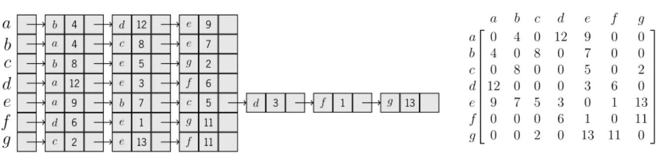
The most common representation seen in the literature is the adjacency list. The graph is represented as an array where each vertex is mapped to an index. Each entry of the array points to a list of destination vertex and weight pairs, representing the edges. This list is usually implemented as a linked-list, allowing the easy manipulation of the graph structure. Alternatively, by using arrays, a more cache friendly approach can be obtained, in detriment of easy of manipulation.
[Bader and Cong, 2004] introduces an extension to the adjacency list representation specifically for Borůvka’s graph contraction algorithm on the CPU: each index can point to multiple lists of incidents
CHAPTER 4. PARALLEL ALGORITHMS AND IMPLEMENTATIONS .. . . b.. 4.. .. d.. 12.. .. e.. 9.. .. . . . . a.. 4.. .. c.. 8.. .. e.. 7.. .. . . . b.. 8.. .. e.. 5.. .. g.. 2.. .. . . . a.. 12.. .. e.. 3.. .. f.. 6.. .. . . . a.. 9.. .. b.. 7.. .. c.. 5.. .. d.. 3.. .. f.. 1.. .. g.. 13.. .. . . . d.. 6.. .. e.. 1.. .. g.. 11.. .. . . . c.. 2.. .. e.. 13.. .. f.. 11.. .. . . a . b . c . d . e . f . g
(a) Adjacency list representation.
a b c d e f g a 0 4 0 12 9 0 0 b 4 0 8 0 7 0 0 c 0 8 0 0 5 0 2 d 12 0 0 0 3 6 0 e 9 7 5 3 0 1 13 f 0 0 0 6 1 0 11 g 0 0 2 0 13 11 0
(b) Adjacency matrix representation.
. . b . d . e . a . c . e . b . e . g . a . e . f . a . b . c . d . f . g . d . e . g . c . e . f . 4 . 12 . 9 . 4 . 8 . 7 . 8 . 5 . 2 . 12 . 3 . 6 . 9 . 7 . 5 . 3 . 1 . 13 . 6 . 1 . 11 . 2 . 13 . 11 . 0 . 1 . 2 . 3 . 4 . 5 . 6 . 7 . 8 . 9 . 10 . 11 . 12 . 13 . 14 . 15 . 16 . 17 . 18 . 19 . 20 . 21 . 22 . 23 . 0 . 3 . 6 . 9 . 12 . 18 . 21 . 3 . 3 . 3 . 3 . 6 . 3 . 3 . a . b . c . d . e . f . g . edge . edge_dst. edge_wt . vertex . first_edge . outdegree (c)CSRrepresentation.
Figure 4.1: Representations of the example graph in Figure1.1.
edges, making it much easier to merge vertice’s edge lists.
The traditional adjacency matrix representation is still widely used. The graph is represented by a matrix
of|V | × |V |, where a value greater than zero in a position (i, j) represents an edge from i to j with the
specified weight. The downside of the adjacency matrix is the large memory requirement. Furthermore, the adjacency matrix stores the information of non-existing edges, making it cumbersome to iterate on the edges, especially for sparse graphs.
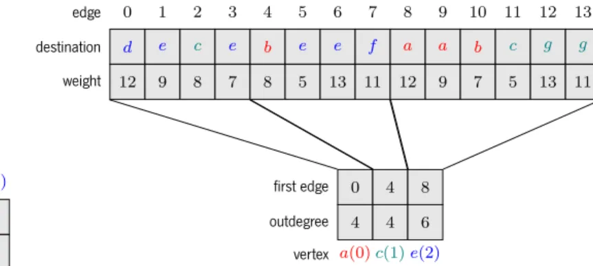
A compromise between the adjacency list and adjacency matrix is theCSRformat and is often seen in the literature as the representation of choice for graph algorithms on theGPU. In this format the graph is represented by four arrays:
• edge_dst- an array of size|E|, which maps each edge to its destination; • edge_wt- an array of size|E|, which maps each edge to its weight; • first_edge- an array of size|V |, which maps each vertex to its first edge;
4.2. LOCK-FREE ADJACENCY LIST
To represent undirected graphs, all edges are duplicated to cover both directions. In the case of the adjacency matrix, the matrix will be symmetric. Figure4.1shows the representations for these three data structures of the example graph in Figure1.1.
In algorithms where the graph structure might change, the usage of adjacency lists is the more attractive approach, asCSRdoes not offer an easy way to alter the graph structure. This comes at a performance cost, since adjacency lists are usually implemented using linked-lists, whileCSRis a more cache friendly approach. However, in Section 4.4 a technique is presented that allows the CSR format to be used in Borůvka’s graph contraction variant.
In this dissertation, theCSRformat will be used to represent the graph, as a way to ensure fairness in the comparison ofCPUand GPUimplementations, and to increase any potential portability of cross-platform algorithms.
4.2 Lock-Free Adjacency List
In some of the algorithms that will be presented in this chapter, there is the need for an efficient way to build theMST. With Prim’s algorithm, one usually resorts an father array: given an arbitrary vertexi, father[i]is the predecessor ofi. The predecessor of the starting vertex is usually the null vertex id, such as-1. Such an array, in a multi-threaded setting, shared among all threads, is not possible, as each vertex can only have a single father, and multiple threads could change the father of a given vertex, resulting in lost edges.
Since the adjacency list is more adequate for building graphs, it can be here instead, as long as adjust-ments are made to make it capable of safe concurrent access. In essence, an adjacency list is an array of linked lists. Implementing a concurrent adjacency list without locks is not possible. However, the only concurrent operation that is needed for this particular adjacency list is insertion at the head of the list, which can be achieved using a single atomic operation.
GNU GCC provides a built-in atomic exchange function, as shown in Listing4.1, which writes the contents of*valinto*ptr, and to original value of*ptrinto*ret.
void __atomic_exchange(type *ptr, type *val, type *ret, int memmodel);
CHAPTER 4. PARALLEL ALGORITHMS AND IMPLEMENTATIONS
Using this function, the insertion of an edge to the head of a linked list can be easily achieved, as shown in Listing4.2. TheEdgestructure is a linked list of edges, and each entry has 3 fields: destination vertex id, edge weight, and a pointer to the next element in the list. TheAdj_List*is an array of the type described above. The operation described in Listing4.2sets the head of the linked list of the specifiedsourcevertex to the newly created edge, while setting the next element of this new edge to the old head of the linked list. void insert_edge(Adj_List *list, unsigned src, unsigned dst, unsigned wt){
Edge *new_edge = (Edge*)malloc(sizeof(Edge)); new_edge->dst = dst;
new_edge->wt = wt;
// Performs the equivalent to this, atomically: // new_edge->next = list[src];
// list[src] = new_edge;
__atomic_exchange(&(list[src]), &new_edge, &(new_edge->next), __ATOMIC_SEQ_CST); }
Listing 4.2: Atomic insertion of an edge into the linked list.
4.3 Multiple Instance Prim
Subsection3.1.3introduced two distinct approaches for parallelizing Prim’s algorithm. In this section, a more in-depth analysis is presented on the multiple instance Prim approach, exploring opportunities for parallelism and identifying limitations. Furthermore, a novel approach, which relies on graph partitioning to assign vertices to each thread, is presented.
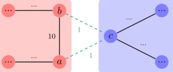
Prim’s algorithm behaves sequentially from its starting vertex, making it possible to run multiple in-stances, in parallel, of Prim growing from different starting vertices [Bader and Cong, 2004, Kang and Bader, 2009,Setia et al., 2009], as illustrated in Figure4.2. As long as the growing trees never touch one other (otherwise known as collisions), they can proceed without interruption. It is state in [Bader and Cong, 2004], that if an instance of Prim is started on every vertex, the algorithm behaves like Borůvka.
In order to maintain the correctness of theMST, whenever a Prim instance tries to add a vertex that belongs to another instance, a collision will occur, and must be handled accordingly. In the provided example, thebluetree will try to add vertex b to its own tree. However, this vertex is marked as belonging to theredtree. The way collisions are treated has a major impact on performance and code complexity.