Assessing riparian vegetation structure and the influence of land use using landscape metrics and geostatistical tools

Contents lists available atScienceDirect

Landscape and Urban Planning

Assessing riparian vegetation structure and the influence of land use using

landscape metrics and geostatistical tools

Maria R. Fernandes

, Francisca C. Aguiar, Maria T. Ferreira

a r t i c l e i n f o

Article history:

Received 22 February 2010

Received in revised form 12 August 2010 Accepted 1 November 2010

Available online 26 November 2010 Keywords: Riparian landscapes Land cover Human influence Spatial patterns Buffer Autocorrelation

a b s t r a c t

Riparian areas are among the most threatened habitats in the world, due to human activities and land use in adjacent areas. In this study we sought to identify landscape metrics for describing the spatial patterns of riparian vegetation affected by land use. We also hypothesize that land use in the immediate vicinity of the riparian area (considered as a 30-m buffer) can have a greater effect on the structure of riparian vegetation than that in an enlarged buffer (i.e. 200 m). The study was conducted in the highly humanized River Tagus watershed (Central Portugal; Western Iberia), along over 80 km of river stretches. Riparian vegetation and land use data were obtained from high-resolution digital images (RGB-NIR 0.5 m× 0.5 m, spring 2005). Patch analyst was used to calculate landscape metrics related to the spatial configuration, isolation, inter-connectivity, and distribution of patches of three riparian cover classes (tree, shrub, and herbaceous). We quantified and accounted for the global and local spatial autocorrelation of data. Data treatment included redundancy analysis and geostatistic methods. Results showed that only a combined interpretation of various landscape metrics can consistently describe the spatial patterns of riparian veg-etation. Riparian vegetation near agricultural areas (irrigation crops, rice fields, orchards, and vineyards), presented a low number of much smaller riparian tree patches with less complex shapes, and a low interspersion of the patch distribution. We found that proximal land use affects the structure of riparian vegetation more than distal land use – an important consideration for the establishment of streamside protection buffers.

© 2010 Elsevier B.V. All rights reserved.

1. Introduction

Riparian zones are responsible for many ecological functions considered crucial to the preservation of river ecological conditions (Forman, 1995; Naiman and Décamps, 1997); they are, however, severely altered due to adjacent human activity and land use, espe-cially in Mediterranean areas (Corbacho et al., 2003; Décamps et al., 1988; Gallego-Fernández et al., 1999; Hooke, 2006; von Schiller et al., 2008). Numerous studies have observed that the composition and spatial patterns of riparian vegetation can be significantly influ-enced by land use (Aguiar and Ferreira, 2005; Allan, 2004; Ferreira et al., 2005; Inoue and Nakagoshi, 2001), but few studies relate the influence of land use at increasing distances from the fluvial sys-tems in rivers and riparian ecosyssys-tems (but seeBott et al., 2006; Bunn and Davies, 2000; McIntyre and Hobbs, 1999).

Stream management and restoration programs have broadly recognized the urgent need to develop methodologies for eval-uating ecological river quality from multiple perspectives. Some

∗ Corresponding author. Tel.: +351 213653380; fax: +351 213653338. E-mail addresses:mrfernandes@isa.utl.pt,rosario.pereira.fernandes@gmail.com (M.R. Fernandes).

studies have focused on floristic composition (Looy et al., 2008), structural and functional attributes, such as the longitudinal and lateral continuity of riparian vegetation (González-del-Tánago and Garcia-Jalón, 2006), percentage of canopy cover, canopy continu-ity, and tree clearing (Aguiar et al., 2009; Johansen and Phinn, 2006), but all of them require intensive field surveys. Other meth-ods are fast and visually based, but do not involve quantification (Dixon et al., 2006; Ward et al., 2003). In other cases, the ripar-ian zone is mapped in a fixed buffer using remotely sensed image data (Congalton et al., 2002; Schuft et al., 1999; Yang, 2007), but the mismatch between the established riparian buffer and the existent riparian zone usually cause errors in the estimation of veg-etation cover. Efficient and quantitative remote measurements of the structure of riparian vegetation are thus needed in watershed studies in order to provide on-the-ground management guidelines for these ecosystems. Image-based methods, satellite images or airborne digital images, become increasingly more cost-effective than field assessments when a higher level of detail is neces-sary (Johansen and Phinn, 2006). Moreover, high spatial resolution imagery (<5 m_{× 5 m pixels) is essential for mapping riparian} veg-etation, due to the limited width of riparian zones and the high spatial variability (Congalton et al., 2002; Davis et al., 2002; Muller, 1997).

0169-2046/$ – see front matter © 2010 Elsevier B.V. All rights reserved. doi:10.1016/j.landurbplan.2010.11.001

Table 1

Structural categories, summary description, acronyms, units and range of landscape metrics; formulae and detailed calculation fromMcGarigal and Marks (1994). Main ecological implications based mainly onForman and Godron (1981)andForman (1995), and applications of landscape metrics to the riparian vegetation.

Structural category Landscape metrics Acronym Units and range Description Main ecological implications

Applications for riparian woods Area/density Number of Patches NP None [1,∞] Basic statistics of the

spatial configuration

Productivity, biogeochemical cycling and species dynamics

Simple indicators of riparian fragmentation Mean Patch Size MPS Square meters

[0,∞] Patch Size Coefficient of Variation PSCV Percentage [0,∞]

Variability in the size of patches

Biological diversity Heterogeneity in the structure of riparian vegetation

Shape Mean Shape Index MSI None [1,∞] Complexity of shapes.

Approaches 1 for shapes with simple perimeters.

Interactions with the adjacent matrix–edge effects Spatial configuration of riparian vegetation, in terms of complexity of riparian patches

Area/edge Mean Fractal

Dimension Index

MPFD None [1,2] Fractal dimension: ratio of perimeter per unit area. Increases as patches become more irregular

Lateral connectivity

Isolation/proximity Mean

Nearest-Neighbor Distance

MNN Meters [0,∞] Minimum distance between patches of the same class, based on the shortest distance between their edges

Flows of energy and biomass and biological diversity–connectivity effects Isolation of riparian patches, inter-connectivity Mean Proximity Index

MPI None [0,∞] Increases as the patches of the corresponding patch type become less isolated and less fragmented.

Ecological neighborhood Degree of isolation and fragmentation of riparian patches

Habitat and refugia discontinuity Contagion/interspersion Interspersion and

Juxtaposition Index

IJI Percentage

[0,100]

Proximity of patches in each class. High values correspond to proportionate distribution of patch type adjacencies Equitability between patches–community dynamics Distribution of riparian patches

Persistence and resilience of communities

The spatial patterns of riparian vegetation can influence eco-logical processes, such as flows of biomass, energy and nutrients, biological diversity and species dynamics (Rex and Malanson, 1990,Turner, 1989). Patches – homogenous areas differing from their surroundings in origin and dynamics – are the fundamen-tal units of landscapes (Forman and Godron, 1981; Wiens, 1976). Helpful tools, such as landscape metrics using Geographical Infor-mation System (GIS) techniques, can characterize the structure of riparian vegetation (Apan et al., 2002). Landscape metrics are numeric descriptors that quantify patch configuration and the spa-tial relationships among patches, such as distribution, isolation and interspersion, and can consequently be used as expressions of ecological processes (Table 1). For instance, the Mean Shape Index – a configuration landscape metric which relates the patch area and its perimeter – can be used to evaluate the edge effect. Convoluted shapes indicate large boundaries, expressing high interactions with the adjacent matrix (Forman, 1995). Reduced connectivity and fragmental patterns indicated by Mean Prox-imity Index and Mean Nearest-Neighbor Distance, particularly in woody vegetation, represent poorer stream ecological conditions (Schuft et al., 1999). Also, the structure of riparian vegetation, the longitudinal continuity of vegetation patches, their aggregation, configuration, expansion limits, and distribution in the riparian zone, can reveal the level of human disturbance and can be used as an indicator of the status of the riparian zone (Johansen et al., 2007).

The traditional statistical approaches to exploring the spatial distribution of vegetation across a landscape generally ignore the

spatial dependence of the data and assume the independence of the samples (Miller et al., 2007). However, one of the basic principles of both geographic and ecological theory is the direct relation-ship between proximity and similarity (Tobler, 1979). The elements that are closer to one another in an ecosystem tend to be influ-enced by the same processes and tend to present a greater degree of likeness (Legendre and Fortin, 1989) – a phenomenon called spatial autocorrelation. Spatial autocorrelation measures the cor-relation of a variable with itself through space, that means the lack of independence between pairs of observation at given distances in space (Legendre, 1993). Disregarding the spatial component in an ecological analysis can lead to erroneous results, since it is a source of bias in most ecological studies. The present study quan-tifies and accounts for the global and local spatial autocorrelation of the data. We mapped riparian patches and land use using air-borne digital images (RGB-NIR spatial resolution 0.5 m× 0.5 m) of impaired landscapes in order to address the following questions:

- Can landscape metrics be used to characterize the structure of riparian vegetation?

- What landscape metrics are most suitable for detecting alter-ations in spatial patterns of riparian vegetation due to land use pressure?

- Does the land use in the immediate vicinity of the riparian zone have more influence on the spatial structure of riparian vegeta-tion than the distal land use?

Fig. 1. Iberian Peninsula, showing the River Tagus watershed (Portuguese part), and the location of the four studied watersheds.

2. Methods

2.1. Site description

The study was conducted on four tributaries along the left margin of the River Tagus (Chouto, Margem, Muge and Sôr) (Fig. 1), all with similar climate and geomorphology. The studied stretches are mostly spread over calcareous Mesozoic formations and have a Mediterranean climate, with a high seasonal vari-ability of rainfall patterns. According to the Atlas do Ambiente (http://www.iambiente.pt/atlas/), the annual runoff ranges from 200 to 300 mm, with an annual average rainfall of 600–800 mm and an annual average temperature of 15–17.5◦C. The land use in the study area is very heterogeneous, including small-scale agri-culture, including orchards, vineyards, maize, pine and eucalyptus forests, Mediterranean shrublands, cork oaklands, and scattered human settlements.

2.2. Field sampling and hydrogeomorphology

Floristic surveys were carried out during the summer of 2004. Sampling sites (n = 15) were 200 m long sections of the river-bank at approximately 3 km intervals along the studied fluvial stretches. We recorded riparian woody species, tree and shrubs, and estimated percentage canopy cover using five classes: (1)<10%,

(2)_{≥10–25%, (3)≥ 25–50%, (4) ≥50–75% and (5) ≥75%. We also} recorded the total number of herbaceous species, and identified the most abundant ones (more than 5% cover).

The hydrogeomorphological characteristics of the streams – namely valley morphology, channel width, dominant substrates of riverbanks, and land use in the floodplain – were obtained from both field observations and GIS layers.

2.3. Structure of the riparian vegetation and land use assessment A GIS was used to store and organize the data obtained from the on-screen photo interpretation of 1:5000 airborne digital images (RGB-NIR spatial resolution 0.5 m× 0.5 m; ortho-rectified and mosaicked, flyover date spring 2005). We studied 21 km of the River Sôr, 33 km of the River Muge, 16 km of the River Margem, and 13 km of the River Chouto.

The riparian zone is defined as the area from the edge of the stream bank to the external visible line of the canopy where an abrupt change in vegetation height, type and amount occurs (Johansen and Phinn, 2006).

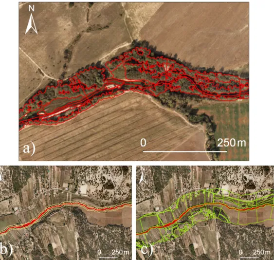
We first divided the river reaches under study into 250 m long sections (sampling units). The lateral limits of the riparian zone were then manually digitalized for both riverbanks (Fig. 2a). Polygons of homogeneous strata of riparian vegetation – riparian patches – were delineated and classified into riparian vegetation

Fig. 2. Illustration of: (a) sampling units and riparian patches, perpendicular lines divide contiguous sampling units, River Sôr; (b) 30 m land use buffer, River Muge; and (c)

200 m land use buffer, River Muge. IGP.

cover classes, within each sampling unit: (i) trees; (ii) shrubs; and (iii) herbaceous. This was done using visual screening of image fea-tures, namely the spatial variation in pixel intensity pattern and the local contrast (gray level differences). Tree cover class had a higher variability in these textural features than the other classes, with the herbaceous class being the most homogenous of all. Areas with shadow were removed from the inner part of riparian patches to capture the overall complexity of their shapes.

Landscape metrics related with the spatial configuration, iso-lation, inter-connectivity, and distribution of riparian vegetation were calculated within each sampling unit for each riparian cover class using the patch analyst – vector format (ArcGis9) extension. Spearman Rank correlations (R) were initially used to evaluate the relationships between the landscape metrics available in the soft-ware. The correlated metrics (|R| > 0.8; p < 0.01) were eliminated to avoid redundancy in the data.Table 1describes the selected land-scape metrics, namely the Number of Patches, Mean Patch Size, Patch Size Coefficient of Variation, Mean Shape Index, Mean Fractal Dimension Index, Mean Nearest-Neighbor Distance, Mean Proxim-ity Index, Interspersion and Juxtaposition Index, as well as their main ecological implications and contribution to the characteriza-tion of the structure of the riparian vegetacharacteriza-tion.

A connectivity distance of 5 m was applied to the Mean Prox-imity Index calculation, as used by Schuft et al. (1999) in the characterization of riparian-stream networks.

Two buffers (30 m and 200 m) were used to evaluate the influ-ence on the riparian vegetation structure of proximal and distal

land use (Fig. 2). Fifty sampling units scattered across the study area were used to identify the existing land uses; for this we used on-screen photo interpretation, along with information from 1:25,000 scale military maps from the Portuguese Army Geographic Institute (www.igeoe.pt). Four land use classes ordered by increasing phys-ical and ecologphys-ical impact in the riparian areas were considered: (1) agroforestry, including oak and cork-oak woodlands, natural pastures, scrublands, fallow ground, extensive crops, and mixed woodland; (2) forestry, including plantations of pine and eucalyp-tus; (3) agriculture, including irrigation crops, rice fields, orchards, and vineyards; and (4) urban, including settlements and industrial areas. The agroforestry class is dominated by the “montados”, a traditional agrosilvopastoral system characterized by long agricul-tural rotations and closed nutrient cycles without fertilizers and pesticides (Plieninger and Wilbrand, 2004). The main ecological consequences of this land use type include the removal of bank vegetation and a decreasing rate of natural regeneration; the other land uses in the study area present manifold and more severe phys-ical and ecologphys-ical consequences for riparian areas and inhabitant communities than the agroforestry class (Table 2).

Patches of land use were delimited for each buffer within each sampling unit. Land use classes were evaluated in terms of percent-age of area occupied, after grouping the patches of the same class. Roads were also taken into account and quantified in length (km) for each sampling unit and land use buffer.

During the summer of 2007, field observations were made in about 25% of the total study area in order to validate the photo

Table 2

Main direct physical effects and potential ecological consequences of the land uses for the riparian areas in the study area.

Land use class Main direct physical effects on the riparian area Potential ecological consequences for the riparian vegetation Agroforestry Bank vegetation removal by grazing Removal of riparian vegetation removed and hampering of natural

regeneration

Forestry Replacement of the riparian woods by forest plantations Reduction of the structural and biological diversity of the riparian woods

Increase in runoff, sediment load and bank erosion by timber extraction

Fragmentation of riparian woods Loss of habitat complexity

Agriculture Superficial water extraction and groundwater pumping Water stress, increased mortality, decreased growth rate and crown volumes of riparian vegetation

Replacement of the riparian woods by agricultural land and irrigation channels

Fragmentation of riparian woods

Inputs of nutrients and pesticides Alteration of the nutrient cycling and imbalance of the inhabitant biological communities

Introduction and excessive growth of exotic species Urban (including

roads)

Increase in runoff and sediments by the impervious surfaces Riparian vegetation stress Riparian habitat reallocation by linearization and channelization

for flood control

Fragmentation of riparian woods Replacement of the riparian habitat by access roads and urban

infrastructures

Pollution and unsuitable conditions for the establishment of riparian vegetation

Alteration of the nutrient cycling and contamination of riparian habitat by pollutants

Introduction of exotic species

interpretation, to confirm the correct allocation of riparian and land use cover classes.

2.4. Spatial autocorrelation assessment

Moran’s I statistics (Moran, 1950) were used to estimate gen-eral patterns of spatial dependency. Moran’s I is frequently used in geostatistical and ecological studies (Fortin et al., 2002; Segurado et al., 2006), and is obtained by dividing the spatial covariation by the total variation of a given attribute. Global Moran’s I evaluates whether the pattern expressed is clustered, dispersed, or random. When the z score indicates statistical significance, a Moran’s I value near +1.0 indicates clustering, while a value near−1.0 indicates dis-persion, and 0 or near to 0 represents no spatial autocorrelation, that means a random pattern.

We calculated Global Moran’s I using three different configu-rations of distance matrices: (i) the “inverse distance criterion”, which includes all the sampling units and gives a lower weight with increasing distances from a given sampling unit; (ii) the “threshold distance”, which only includes the sampling units within a dis-tance of 1000 m; and (iii) the “first continuity order”, which only includes the sampling units that share boundaries, the left and right contiguous sampling units.

A semivariogram function (Cressie, 1991; Wackernagel, 2003; Webster and Oliver, 2007) was applied to the riparian vegetation data, for the four streams, in order to calculate the spatial inde-pendence distance between sampling units. A variogram function is a mathematical description that relates the variance (or dissim-ilarity) of samples from a given attribute with the distance that separates them (Isaacs and Srivastava, 1989). Because nearby sam-ples tend to have similar attribute values, low variance among samples is expected in the semivariogram. The variance increases asymptotically to the limit value, as the distances between samples increase. Samples that are separated by distances below this limit are spatially autocorrelated, whereas samples that are farther apart are independent, because the expected variance is not significantly different from the asymptotic value. The distance value between samples at which spatial autocorrelation is considered insignificant is named “range” (Oline and Grant, 2002).

We also calculated the Local Moran’s I (Anselin, 1995) – a measure of contagion that includes the effect of the spatial neigh-borhood (Keitt et al., 2002; Segurado and Araújo, 2004). The Local

Moran’s I have a spatial autocorrelation value for each sampling unit, rather than the single value of the Global Moran’s I.

The spatial dependence of the land use variables was not eval-uated, because ensuring the spatial independence of the biological variable means that unbiased correlations between dependent and independent variables are guaranteed (Lennon, 2000).

2.5. Influence of land use on the structure of riparian vegetation Constrained ordination procedures were performed in CANOCO version 4.5 (ter Braak and Smilauer, 2002) to determine the influ-ence of land use on the structure of the riparian vegetation (n = 330 sampling units). The gradient lengths of the landscape metrics datasets were evaluated with Detrended Correspondence Analy-sis. As the gradient lengths were lower than 4 standard deviation units (Leps and Smilauer, 2003) thus indicating a linear response, Redundancy Analysis (RDA) was used.

The effect of the spatial component in our data was analysed using two approaches: (1) by incorporating the spatial component into the landscape metrics dataset; and (2) by removing the spatial autocorrelation. For the first approach, RDA runs were performed: (i) using just land use variables; (ii) using land use variables and the Local Moran’s I matrix as co-variable (i.e. spatial variables); and (iii) using the spatial and the land use variables together.

For the second approach, we performed RDA using spatially independent sampling units. The distance between sampling units was defined by the “range” values obtained by the application of a semivariogram function to the landscape metrics (see Section 2.4). The subsampling method was defined to maximize the sam-ple size, and avoided the duplication of any sampling unit. More precisely, the independent subsamples were obtained by systemat-ically using an sampling unit that was separated from the following one by the “range” value: for instance, the first subsample begins with the inclusion of sampling unit1, the second subsample begins in sampling unit2, and so forth.

In both approaches the landscape metric datasets for the three riparian cover classes were centred and standardized and the cor-relation matrix was used to make them comparable. RDA runs were performed with forward selection of land use variables, and unre-stricted Monte Carlo permutation tests for each one. A cut-off point of 0.10 was adopted. Variance inflation factors were examined to detect co-linearity between the land use variables. The total

vari-Table 3

Minimum and maximum values of landscape metrics; average (± SD) for each riparian cover class (n = 330 sampling units). Acronyms for landscape metrics are given in Table 1. Dominant riparian taxa, observed percentage cover class in parentheses, average species richness± SD for the tree, shrub and herbaceous cover classes (n = 15 field surveys).

Riparian cover classes

Tree Shrub Herbaceous

Landscape metrics NP 1.00–14.00 (3.43± 2.29) 1.00–11.00 (2.23± 1.62) 1.00–8.00 (1.92± 1.12) MPS 21.67–11268.02 (1000.57± 1387.17) 5.41–4770.42 (413.94± 626.97) 6.73–2183.67 (420.70± 501.30) PSCV 6.60–211.81 (84.29± 41.10) 2.67–151.54 (63.20± 34.03) 9.01–128.58 (57.57± 30.49) MSI 1.03–5.47 (2.00± 0.76) 1.08–4.15 (1.79± 0.57) 1.16–5.70 (2.12± 0.93) MPFD 1.47–2.13 (1.69± 0.11) 1.46–2.67 (1.73± 0.17) 1.45–2.69 (1.78± 0.17) MNN 0.37–171.70 (15.10± 23.94) 0.80–210.70 (34.49± 45.13) 1.80–134.50 (28.35± 29.29) MPI 2.43–4584.94 (379.34± 651.59) 1.12–539.37 (81.96± 126.11) 2.26–114.37 (25.35± 28.15) IJI 0–22.66 (10.00± 5.37) 1.27–24.99 (11.63± 4.89) 0–19.97(8.91± 5.71) Floristic composition

Dominant taxa (cover class)

Salix salviifolia (3) Sambucus nigra (2) Juncus sp.

Salix atrocinerea (3) Rubus ulmifolius (1) Scirpus holoschoenus

Fraxinus angustifolia (3) Crataegus monogyna (1) Cyperus longus

Populus nigra (2) Tamarix africana (1) Agrostis stolonifera

Alnus glutinosa (2) Frangula alnus (1) Mentha suaveolens

Salix alba (1) Holcus lanatus

Average species richness (± SD) 4± 1.3 1.2± 1 25± 6.5

ance – also called ‘total inertia’ – explained by each combination was obtained by the sum of all canonical unconstrained eigenvalues (ter Braak and Smilauer, 2002).

Multiple linear regressions were performed to evaluate the rela-tionship between the various types of land use and the landscape metrics. To identify the land use classes that contributed most to explaining the structure of the riparian vegetation, we used for-ward selection procedures and counted the number of significant regressions (p < 0.05) per land use class and land use buffer, for each landscape metric. STATISTICA software version 6.0 (StatSoft Inc., 2001) was used for the regression analyses.

In addition, we compared the expected and the observed responses of the landscape metrics to land use. Bibliographic sources, such asAguiar et al. (2000),Aguiar and Ferreira (2005), Guirado et al. (2007), Schuft et al. (1999), Shandas and Alberti (2009),Timm et al. (2004),Wu et al. (2000), and expert judgment were used to suggest the behaviour, positive or negative relation-ships, of the landscape metrics influenced by land use.

3. Results

3.1. Riparian composition and hydrogeomorphology

Stretches of the Margem and the Chouto and the upstream section of the Sôr are of medium valley width. The riparian for-mations are dominated by willows, namely Salix salviifolia and Salix atrocinerea. The deep soils of the downstream section of the Margem support riparian woods dominated by ashes (Fraxinus angustifolia) and alders (Alnus glutinosa). The shrub strata is domi-nated by hawthorns (Crataegus monogyna), black elders (Sambucus nigra), and alder buckthorns (Frangula alnus). Tamarix africana was found in the most near-natural upstream section of the River Sôr. A patch mosaic of small-scale agriculture including orchards, vine-yards and maize, and scattered human settlements dominated the landscape of these valleys.

The Rivers Muge and Sôr presented a relatively larger valley and channel width than the previous rivers, and their downstream sections often presented sand bars. Riparian woods were mainly composed of willows, and occasionally ashes and hawthorn. Iso-lated groups of black poplar (Populus nigra) were also found in the middle section of the Sôr. The most degraded areas were frequently composed of a sole shrub strata of Salix sp., surrounded by sedges of bramble ticket (Rubus ulmifolius) Eroded embankments with fine substrates were frequently invaded by the giant reed (Arundo

donax). Large regular patches of rice, maize and other irrigation crops dominated the landscape near the riparian zone.

The natural regeneration of ashes and willows was frequently observed in the inner banks.

Forests of Mediterranean shrublands, cork oaklands, and pine and eucalyptus forests were widespread on the floodplain. 3.2. Structure of riparian vegetation

The study area encompassed 330 sampling units, which resulted in the delimitation of 3900 patches of riparian vegetation.

Table 3summarizes the overall characteristics of the structure of the riparian vegetation using landscape metrics and the dominant taxa found for each cover class. The tree cover class was mostly composed of willows, ashes and alders. This class was the most abundant, and presented the largest riparian patches (Mean Patch Size values) when compared to the other riparian cover classes, although a higher variability of the patch size (Patch Size Coef-ficient of Variation values) was also found. The highest number of tree cover patches (Number of Patches values) was found in the upstream sampling units of the River Sôr, whereas lower val-ues occurred close to urban areas and small farms, or associated with areas with large widths of riparian vegetation, at least more than 30 m. Landscape metrics associated with the connectivity – namely the Mean Nearest-Neighbor Distance and the Mean Prox-imity Index – provide evidence of a higher connectivity of tree cover class in comparison to the other riparian cover classes. The high Mean Fractal Dimension Index values found for this ripar-ian cover class corresponded to complex shapes with meandering forms, associated with large riparian widths. We even found a small number of riparian tree patches with Mean Fractal Dimension Index values that exceeded the maximum value usually referred to in the literature (seeTable 1).

Riparian shrub strata frequently included black elder, hawthorn and dyer’s buckthorn. Patches of shrubs were smaller than the tree patches, but presented less fragmentation.

Under the canopies, the vegetation was dominated by a commu-nity of grasses, reeds, rushes and other vascular species associated with wet environments.

Where the herbaceous cover class was concerned, higher Mean Patch Size (MPS) values occurred near irrigation crops or associ-ated with temporary sand deposits; also, higher Mean Shape Index (MSI) values were associated with elongated shapes, which were a frequent characteristic of this riparian cover class.

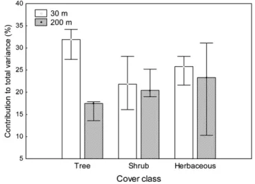
Fig. 3. RDA results expressed by the contribution of land use variables to explaining

the total variance of riparian cover classes, using three approaches: (1) solely land use variables, (2) land use variables and spatial co-variables, and (3) land use and spatial variables, with the 30 m and 200 m land use buffers (330 sampling units).

All riparian cover classes presented low Interspersion and Juxta-position Index values, meaning that the riparian patches were not proportionately distributed in the study area.

The classification by on-screen photo interpretation agreed with the field observations. The few differences that were found were related to recent local disturbances, such as vegetation removal due to sand extraction.

3.3. Spatial autocorrelation assessment

The results of the Global Moran’s I and its statistical significance for the three configurations of the distance matrix indicated the presence of spatial autocorrelation in most of the landscape metrics across the studied area (Appendix 1). The Mean Proximity Index had a spatial random pattern, except for the shrub cover class; nor did the Mean Nearest-Neighbor Distance reveal a significant clustered pattern for any of the riparian cover classes. No clear dispersed patterns were found. We observed clear differences in the spatial patterns for the riparian cover classes using the various configura-tions of the distance matrix, which indicates the existence of local spatial autocorrelation patterns. In addition, when the restriction of the sampling unit neighborhood was applied to the tree cover class, with a threshold distance and first continuity order approaches, we observed a higher spatial autocorrelation value than using the inverse distance criteria, which included all the sampling units. This means that the tree cover class had a higher spatial dependence at a local level than at the global level.

The application of a semivariogram function to the landscape metrics for the four streams resulted in an estimation of the “range” value that varied between 2395 m and 2963 m. In order to ensure that sampling units were spatially independent, we therefore used the value of 3000 m between sampling units. The subsampling resulted in 9 combinations (n = 28) of different sampling units (see Section2.5for detailed subsampling method).

3.4. Influence of land use on the structure of riparian vegetation Fig. 3shows the results of the contribution of the land use vari-ables to the total variance of the structure of the riparian vegetation obtained from the RDA runs for the three approaches.

On the whole, the explained variance using the proximal land use (30 m land use buffer) presented consistently higher values than that using the distal land use (200 m land use buffer). This

Fig. 4. Average, minimum and maximum RDA results expressed by the contribution

of land use variables to explaining the total variance of riparian cover classes, using spatial independent sampling units (28 sampling units per subsample) for the 30 m and 200 m land use buffers.

pattern was also observed for stream sections with slightly differ-ent valley morphologies, namely the Margem/Chouto and Muge/ Sôr.

Another consistent pattern that emerges in the overall RDA anal-yses was the decrease in the explained variance upon removal of the spatial component (Local Moran’s I as co-variable). The explained variance that results from using the spatial and the land use vari-ables together, ranged from 20.1% to 33.4%. These results indicate that the structure of the riparian vegetation is more dependent on its spatial component than on the land use variables from either buffer. This means that part of the variance of the riparian vegeta-tion is explained by neighboring values. We also observed higher total variance for the tree cover class than for the other riparian cover classes.

Fig. 4illustrates the contribution of land use variables, prox-imal and distal land use buffers, to an explanation of the total variance of the riparian cover classes, using combinations of spa-tially independent sampling units (9 subsamples; 28 sampling units per subsample). We observed a high increase of the total variance when compared with the previous approach, where we used non-independent sampling units (Fig. 3). Likewise, the proximal land use buffer had a greater influence on the overall riparian cover classes than the distal land use buffer. This trend was especially evident for the tree cover class. For the herbaceous cover class, a high variability was detected in relation to the results of the 9 RDAs we performed.

3.5. Influence of land use classes on the tree cover class

We used the tree cover class to evaluate the influence of the different land use classes, since it was best represented in the study area and displayed the highest percentage of variance explained by land use variables, compared to the other cover classes (Figs. 3 and 4).

Using both early findings from the literature and expert judge-ment, we suggested a negative relationship between most of the landscape metric values and the tree cover class when influenced by human land use, except in the case of the Mean Nearest-Neighbor Distance, and Number of Patches (Table 4). We therefore expected that increasing land use pressure would result in a high num-ber of patches (expressed by Numnum-ber of Patches), and smaller patches (expressed by Mean Patch size) with less complex shapes (expressed by low Mean Fractal Dimension Index values, and low

Table 4

Expected and observed responses of landscape metrics to the increasing areas occupied by each land use (↑-positive relation; ↓-negative relation) for the tree cover class. Number of significant multiple regression analyses (p < 0.05) of landscape metrics and land use variables (30 m and 200 m land use buffers) using spatial independent sampling units (9 subsamples; 28 sampling units per subsample). Acronyms for landscape metrics are given inTable 1.

Landscape metrics Expected response Observed response

Agroforestry Forestry Agriculture Urban Roads

30 m 200 m 30 m 200 m 30 m 200 m 30 m 200 m 30 m 200 m NP ↑ ↑ 1 ↓ 5 ↓ 1 ↓ 1 MPS ↓ ↓ 3 ↓ 7 PSCV ↓ ↓ 1 ↓1 ↓ 1 ↓ 4 ↓ 1 ↑ 1 MSI ↓ ↓ 2 ↓ 6 ↓ 1 MPFD ↓ ↓ 1 ↓ 1 ↓ 1 ↓ 3 ↓ 1 ↓ 1 MNN ↑ ↑ 2 ↓ 1 ↑1 ↑ 1 ↑ 1 ↑ 1 MPI ↓ ↑ 1 ↓ 1 ↓ 2 ↓ 1 ↓ 1 ↑ 1 IJI ↓ ↓ 2 ↑1 ↓ 7 ↓ 1 ↓ 1 ↓ 2 ↑ 1

Mean Shape Index values), but more isolated patches (high Mean Nearest-Neighbor Distance values and low Mean Proximity Index values). We also expected more homogeneous riparian patches, (expressed by lower Patch Size Coefficient of Variation values), and low interspersion of the patch distribution (expressed by low Inter-spersion and Juxtaposition Index values) along a gradient of land use pressure.

In general, the observed responses of the landscape metrics were concordant with the expected ones (Table 4). Agricul-ture presented the highest number of significant regressions (p-value < 0.05) with virtually all the landscape metrics, the excep-tion being the fragmentaexcep-tion metrics Mean Nearest-Neighbor Distance and Mean Proximity Index. We observed a low number of much smaller riparian tree patches, with less jagged shapes, and a low interspersion of the patch distribution with increasing agri-cultural areas in the land use buffer – mainly in the 30 m buffer. For the other land uses the general patterns of degradation were similar to those found for agriculture, though supported by a low number of significant responses. We also observed an increase in

the degradation pattern across the land use pressure gradient, from agroforestry to urban land use (Fig. 5).

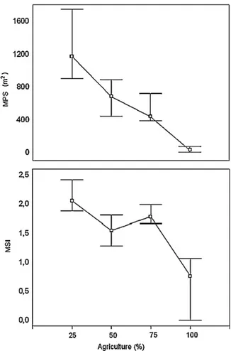
We selected two landscape metrics with a high number of sig-nificant regressions with the agriculture in the 30 m land use buffer, to illustrate the response of the landscape metrics to the increase of the agricultural area (Fig. 6). The Mean Patch Size presented lower values and low variability with the increasing agricultural area. The same pattern was observed for the Mean Shape Index, albeit with higher variability with increasing agricultural areas.

4. Discussion

4.1. Structure of the riparian vegetation

Numerous studies on the ecology and management of riparian zones seek to relate human disturbances in the surrounding land-scapes with degradation of riparian vegetation (Baker et al., 2007; Malanson and Cramer, 1999). The use of field-based methods over large riparian areas is very time-consuming and often results in the

Fig. 5. Values of the landscape metrics for the tree cover class with adjacent land use of: (a) agriculture, River Chouto; (b) agroforestry, River Chouto; and (c) forestry and

Fig. 6. Median, 25, and 75 quartiles for the Mean Patch Size (MPS) and Mean Shape

Index (MSI) for the tree cover class with the increase of the agricultural areas in the 30 m buffer (9 subsamples; 28 sampling units per subsample).

loss of the overall perception of the landscape, making it difficult to propose management guidelines, like forestation of degraded areas, stock management, establishment of riparian buffers, con-trol of invasive plants, or to help managers prioritize the places to restore, improve, or protect. Landscape metrics, such as Mean Patch Size, Mean Nearest-Neighbor Distance, or Mean Proximity Index, can be used as proxies of riparian width, longitudinal continuity and fragmentation (Johansen and Phinn, 2006), and therefore indi-cate the status of the riparian vegetation. The present study uses a set of landscape metrics and proposes a combined approach in order to characterize the structure of the riparian vegetation. It is widely recognized that combining landscape metrics from the same category, such as the Number of Patches and Mean Patch Size (Apan et al., 2002), is necessary for there to be a reliable evaluation of the structure of riparian vegetation.

In addition to confirming this, the present study points to the advantage of a complementary approach using landscape metrics from diverse categories. For instance, the joint use of area/density and shape metrics, such as the Number of Patches and Mean Shape Index, and metrics of connectivity (e.g. Mean Nearest-Neighbor Dis-tance, Mean Proximity Index), helps characterize the structure of riparian vegetation. This was the case with wide well-preserved riparian vegetation stretches, which consistently displayed large connected tree patches with complex shapes, whereas herbaceous vegetation was characterized by elongated and connected patches with simple shapes. These findings can also help to identify highly degraded riparian zones, such as those in Portugal’s coastal water-sheds, which are invaded by the alien species Arundo donax L. (giant reed). The giant reed forms dense, monotypic stands, and thus high connected patches, but with simple stretched shapes, which can be

identified using a combination of landscape metrics like the Mean Nearest-Neighbor Distance, Mean Proximity Index, Mean Shape Index and Number of Patches. However, knowledge of the hydroge-omorphological background of watercourses is still indispensable, since the narrow riparian zones that are naturally found in first-order streams mimic the degraded riparian vegetation, with small linear patches and low inter-connectivity.

The shrub and herbaceous cover classes were naturally under-estimated, due to the superimposition of canopies. However, distinguishing between the tree and shrub cover classes is feasible using the type of high-resolution images to which we had access. Most studies using remote sensing have only considered the ripar-ian woody vegetation, shrubs and trees (Apan et al., 2002; Schuft et al., 1999). Whereas for more detailed assessments, it is neces-sary to characterize the canopy and subcanopy surface topography, and other remote sensing techniques, such as the LIDAR sensors, broad beam, full return with high sampling rates (Goetz, 2006), are recommended.

4.2. Spatial autocorrelation assessment

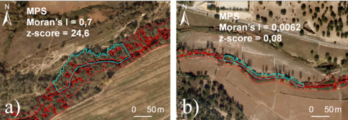
This work also points to the importance of quantifying and taking into account the spatial component of the data, which is particularly relevant in riparian vegetation studies, due to its linear nature. In the present study most of the landscape metrics revealed a high global spatial autocorrelation, and also local patterns of spatial dependence. By mapping the Local Moran’s I it is possi-ble to identify the sampling units with highest spatial dependence (Fig. 7a) and spatial independence (Fig. 7b), per landscape met-ric, which can provide site-specific information for management of degraded areas. Exceptionally, the connectivity metric Mean Proximity Index showed a spatially random pattern for the tree cover class; however, this could be explained by the selection of the connectivity threshold (5 m), rather than by spatial indepen-dence of data distribution. The spatial autocorrelation patterns we observed can be explained by historical factors (Dormann, 2007; Segurado et al., 2006), or biotic factors (Legendre, 1993), or envi-ronmental variables (Legendre and Fortin, 1989). This study also suggests a spatial autocorrelation evaluation procedure for the influence of the surrounding land use in the riparian structure, using two approaches: incorporation of the spatial component; and the use of spatially independent Sampling Units. The former procedure revealed a high dependency of the data on the spatial component, and a decrease in the extent to which land use vari-ables helped explain the total variance of the structure of riparian vegetation. The second approach, by removing the spatial autocor-relation, led to a significant increase in the variance explained by land use, although we inevitably lost biological information due to subsampling.

4.3. Influence of land use in the structure of the riparian vegetation

In general, there was an agreement between the expected and the observed responses of the landscape metrics due to the influ-ence of land use. The present study clearly showed that riparian tree patches affected by nearby agricultural areas are characterized by a low number of small patches, whereas in the riparian areas of Cedar River, USA,Timm et al. (2004)observed degraded riparian areas with numerous small patches. For management purposes, a clear referential of well-preserved riparian vegetation in the region is therefore needed in order to define the near-natural spatial pat-terns and to further identify possible changes due to land use. This result can be also due to different magnitudes of land use pressure; thus low numbers of small patches in our area can be indicative of a highly degraded landscape. In contrast to our results,Apan et al. (2002)did not observe differences in patch configurations

Fig. 7. Morans’ I and z-score for the Mean Patch Size (MPS) for the tree cover class. Illustration of: (a) high spatial dependence (River Sôr); and (b) spatial independence

(River Muge).

(namely Mean Shape Index and Mean Fractal Dimension Index val-ues), possibly due to the coarse resolution of the mapping resources (Baker et al., 2007). The low representation of the remaining land use classes in the study area did not make it possible to achieve a consistent pattern in the relationships between the land uses and the structure of riparian vegetation. Nevertheless, the values of the landscape metrics point towards the degradation of the riparian vegetation along the land use pressure gradient, from agroforestry to urban land uses.

This study found that the proximal land use has a greater effect on the structure of the riparian vegetation than distal land use, as has been suggested by studies in other geographic areas (Bott et al., 2006; Bunn and Davies, 2000; von Schiller et al., 2008) and by a precursor study in the River Tagus watershed byFerreira et al. (2005). The latter stated that the “proximity and extension of land use patches interplay to influence the degree of changes in the riparian areas”. In fact, an increment of around 14% of explained variance was achieved at the 30 m land use buffer, compared to the distal land use buffer. Even so, a large part of the variability in the structure of the riparian vegetation remained unexplained. Natural disturbances, such as fire, and the flash-flow hydrologi-cal regime typihydrologi-cal of Mediterranean rivers, as well as site-specific human disturbances, such as tree clearing, sand extraction, and channel re-profiling, can help to explain part of the structure of riparian vegetation (McIntyre and Hobbs, 1999). The composition of riparian vegetation, especially the tree and shrub cover classes, could also partially explain the variability of the spatial patterns of riparian vegetation, and it is essential to detect non-native vege-tation patches. We therefore advocate a comprehensive approach to the evaluation of the conservation status of riparian vegetation, which should be based on the interpretation of a set of landscape metrics and supported by a posteriori on-ground vegetation survey methods.

5. Conclusions and implications for riparian management

The structure of riparian vegetation can give essential clues for riparian management, and its assessment through landscape metrics can help prioritize where to restore, enhance, or protect riparian zones. Below we present the main findings of the present study and their implications for riparian management:

5.1. Spatial patterns of riparian vegetation can be consistently described with a combination of landscape metrics from various categories

Although it is important to use various configuration, isolation, fragmentation and distribution-based landscape metrics to assess

degradation in detail, the ultimate selection of landscape metrics rely on the management or conservation goals in question. In cer-tain situations, only one or two metrics are necessary. For instance, the Mean Proximity Index can be used to restore the longitudinal connectivity of riparian corridors for the movement or dispersal of a given target-species. A threshold distance for the species is defined a priori as the minimum distance between patches required for the use of the riparian area as an ecological corridor. The stretches that need to be restored are identified when the metric value is zero. For a quick identification of fragmented areas, the Mean Nearest-Neighbor Distance combined with the Mean Patch Size can give an idea of the overall degradation. On the other hand, when seeking to identify which riparian areas to protect, we suggest the use of spatial configuration metrics associated with ecological fluxes and species dynamics, such as the Mean Shape Index, Mean Patch Size and Mean Fractal Dimension Index, combined with metrics that evaluate fragmentation. The results of landscape metrics can be easily mapped on a GIS platform, thereby allowing the visualiza-tion of critical areas, and can also be used to monitor the success of the restoration or conservation actions.

High spatial resolution imagery – pixel size less than five metres – is required in order to assess the structure of riparian vegetation, and principally for the spatial configuration metrics Mean Shape Index and Mean Fractal Dimension Index. This resolution is needed to capture the complexity of the shape of riparian patches. Besides spatial resolution, other characteristics of the images must be con-sidered. The radiometric resolution, which is the number of digital levels used to express the data collected by the sensor, should pos-sess a minimum of eight bits (0–255 digital numbers). Otherwise the discrimination of the riparian cover classes by the perception of the grey level scale will be impaired. Where spectral resolution – the width and the number of the spectral bands of the sensor – is concerned, a “true color image” given by the combination of the blue, green and red bands in the visible region is appropriate to the application of this approach, since it does not make use of the numerical information in the bands.

5.2. Proximal land use has a greater effect on the structure of riparian vegetation than distal land use, especially in areas occupied by agriculture

Understanding the importance of the land uses and related human activities in river surroundings can undoubtedly help take practical managerial decisions. In Portugal there are no legislative tools that are specifically designed to limit the human pressures near riparian zones. The width of streamside public areas depends solely on the size of catchment areas. Protection buffers ought to take account of the impact of the different land uses on the river

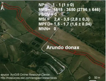
sur-Fig. 8. Invasion of riverbanks by the giant reed; minimum and maximum values of

landscape metrics; average± SD in parentheses for giant reed patches (16 sampling units at River Aveiras, 4 km).

“World User Imagery” from the ArcGIS Resourcer Center (http://www.resources. esri.com/arcgisonlineservices), spatial resolution 1–2 m.

roundings and include measures that restrict access to the riparian area, sand extraction from riverbanks, and clear-cuts of riparian vegetation. Where possible, ecologically sustainable land uses in the proximity of the riparian area, such as the traditional agro-forestry systems, must be encouraged.

5.3. The pattern of degradation of riparian vegetation is characterized by a reduction in the number, size and complexity of riparian tree patches, along with a disproportionate patch distribution within the riparian landscape

One of the main contributions made by the present study was the characterization of the spatial patterns of the structure of ripar-ian vegetation when impacted by land use. However, caution must be observed: (i) when transposing the present results to other regions; it is crucial to define a structural benchmark by assess-ing the patterns of near-natural riparian vegetation which is as unimpaired by human land use and other pressures as possible; (ii) with riparian areas invaded by alien, or composed of forestry species; in general, it is to be expected that connected and large riparian patches will correspond to well-preserved riparian areas, but they can be the result of monospecific stands of non-riparian or non-native species; (iii) with the spatial component of data; spatial autocorrelation can influence the results obtained when assessing effects of land use.

5.4. Additional outcomes of the present study for riparian management

Landscape metrics can be used to identify areas invaded by alien plants, such as those caused by the giant reed. The present approach is being improved for detecting and mapping invaded areas by the use of the spectral reflectance signature of this species. The giant reed form usually simple, large and elongated patches, that extend in continuous and almost monospecific stands along riverbanks (Fig. 8).

The present study also provided evidence that using just the tree cover class to characterize the structural features of woody ripar-ian vegetation does not lead to a substantial loss of information. This has the advantage of being less time-consuming, especially in digitalizing the riparian patches, and also overcomes the problem of underestimated shrubby canopies.

Mapping the spatial autocorrelation of the riparian vegeta-tion can provide addivegeta-tional management informavegeta-tion. Riparian stretches that present autocorrelation can be object of the same management actions. It is to be expected that the vegetation struc-ture along stretches that present spatial dependence will present similar responses to managerial activities, such as the restoration of longitudinal connectivity. The detection of local autocorrelation patterns can help locate site-specific riparian areas with similar patterns in the contiguous adjacencies within the riparian area, and also areas of transition with regard to changes in structural fea-tures, such as the fragmentation or diverse distribution of riparian patches.

Acknowledgements

This study received backing from the project RIPIDURABLE “Gestion Durable de Ripisylves” (INTERREG III-C Sul - 3S0125I), and from the Forest Research Centre, CEF through FEDER/POCI 2010. Maria R. Fernandes and Francisca C. Aguiar were supported by doctoral and post-doctoral scholarships from the Foundation for Science and Technology, Portugal, SFRH/BPD/29333/2006 and SFRH/BD/44707/2008, respectively. We acknowledge the Instituto Geográfico Português (IGP), which provided the airborne digital images through the FIGEE program. Thanks are also due to Pedro Segurado for suggestions concerning methods for estimating the spatial autocorrelation.

Appendix A. Supplementary data

Supplementary data associated with this article can be found, in the online version, atdoi:10.1016/j.landurbplan.2010.11.001.

References

Aguiar, F.C., Ferreira, M.T., 2005. Human-disturbed landscapes: effects on composi-tion and integrity of riparian woody vegetacomposi-tion in the Tagus River basin, Portugal. Environ. Conserv. 32 (1), 30–41.

Aguiar, F.C., Ferreira, M.T., Moreira, I., Albuquerque, A., 2000. Riparian types in Mediterranean basin. Aspects Appl. Biol. 58, 221–232.

Aguiar, F.C., Ferreira, M.T., Albuquerque, A., Rodriguez-Gonzalez, P., Segurado, P., 2009. Structural and functional responses of riparian vegetation to human disturbance: performance and scale-dependence. Fundam. Appl. Limnol. 175, 249–267.

Allan, J.D., 2004. Landscapes and riverscapes: the influence of land use on stream ecosystems. Ann. Rev. Ecol. Syst. 35, 257–284.

Anselin, L., 1995. Local indicators of spatial association-LISA. Geogr. Anal. 27, 93–115. Apan, A.A., Raine, S.R., Paterson, M.S., 2002. Mapping an analysis of changes in the riparian landscape structure of Lockyer Valley catchment Queensland, Australia. Landscape Urban Plan. 59, 43–57.

Baker, M.E., Weller, D.E., Jordan, T.E., 2007. Effects of stream map resolution on mea-sures of riparian buffer distribution and nutrient potential. Landscape Ecol. 27 (7), 973–992.

Bott, T.L., Montgomery, D.S., Newbold, J.D., Arscott, D.B., Dow, C.L., Aufdenkampe, A.K., Jackson, J.K., Kaplan, L.A., 2006. Ecosystem metabolism in streams of the Catskill Mountains (Delaware and Hudson River watersheds) and Lower Hudson Valley. J. N. Am. Benthol. Soc. 25, 1018–1044.

Bunn, S.E., Davies, P.M., 2000. Biological processes in running waters and their impli-cations for the assessment of ecological integrity. Hydrobiologia 442/443, 61–70. Congalton, R.G., Birch, K., Jones, R., Schriever, J., 2002. Evaluating remotely sensed techniques for mapping riparian vegetation. Comput. Electron. Agric. 37, 113–126.

Corbacho, C., Sánchez, J.M., Costillo, E., 2003. Patterns of structural complexity and human disturbance of riparian vegetation in agricultural landscapes of Mediter-ranean area. Agric. Ecosyst. Environ. 95, 495–507.

Cressie, N., 1991. Statistics for Spatial Data. John Wiley and Sons, New York. Davis, P.A., Staid, M.I., Plescia, J.B., Johnson, J.R., 2002. Evaluation of Airborne Image

Data for Mapping Riparian Vegetation within the Grand Canyon. Report of U.S Geological Survey, Arizona.

Décamps, H., Fortune, M., Gazelle, F., Patou, G., 1988. Historical influence of man on the riparian dynamics of fluvial landscape. Landscape Ecol. 1, 163–173. Dixon, I., Douglas, M., Dowe, J., Burrows, D., 2006. Tropical Rapid Appraisal of

Ripar-ian Condition Version 1. River Management Technical Guidelines. No.7 Land and Water Australia, Canberra, Australia.

Dormann, C.F., 2007. Effects of incorporating spatial autocorrelation into the analysis of species distribution data. Global Ecol. Biogeogr. 16, 129–138.

Ferreira, M.T., Aguiar, F.C., Nogueira, C., 2005. Changes in riparian woods over space and time: influence of environment and land use. Forest Ecol. Manage. 212 (1–3), 145–159.

Forman, R.T.T., 1995. Land Mosaics: The Ecology of Landscapes and Regions. Cam-bridge University Press, CamCam-bridge.

Forman, R.T.T., Godron, M., 1981. Patches and structural components for a landscape ecology. Bioscience 31, 733–740.

Fortin, M.-J., Dale, M.R.T., Hoef, J., 2002. Spatial analysis in ecology. Encyclopedia of Environmetrics, 4. John Wiley Sons, Ltd., Chichester, pp. 2051–2058. Gallego-Fernández, J.B., García-Mora, M.R., García-Novo, F., 1999. Small wetlands

lost: a biological conservation hazard in Mediterranean landscapes. Environ. Conserv. 26 (3), 190–199.

Goetz, S.J., 2006. Remote sensing of riparian buffers: past progress and future prospects. J. Am. Water Resour. Assoc. 2, 133–143.

González-del-Tánago, M., Garcia-Jalón, D., 2006. Attributes for assessing the envi-ronmental quality of riparian zones. Limnetica 25 (1–2), 389–402.

Guirado, M., Pino, J., Roda, F., 2007. Comparing the role of site disturbance and landscape properties on understory species richness in fragmented periurban Mediterranean forests. Landscape Ecol. 22, 117–129.

Hooke, J.M., 2006. Human impacts on fluvial systems in the Mediterranean region. Geomorphology 79, 311–335.

Inoue, M., Nakagoshi, M., 2001. The effects of human impact on spatial structure of the riparian vegetation along the Ashida river, Japan. Landscape Urban Plan. 53, 111–121.

Isaacs, E.H., Srivastava, M., 1989. An Introduction to Applied Geostatistics. Oxford University Press, New York, p. 146.

Johansen, K., Phinn, S., 2006. Mapping structural parameters and species composi-tion of riparian vegetacomposi-tion using IKONOS and Landsat ETM+ Data in Australian Tropical Savannahs. Photogramm. Eng. Remote Sens. 72 (1), 71–80.

Johansen, K., Coops, N.C., Gergel, S.E., Stange, Y., 2007. Application of high spatial res-olution satellite imagery for riparian and forest ecosystem classification. Remote Sens. Environ. 110 (1), 29–44.

Keitt, T.H., Bjornstad, O.N., Dixon, P.M., Citron-Pousty, S., 2002. Accounting for spa-tial pattern when modelling organism–environment interactions. Ecography 25, 616–625.

Legendre, P., 1993. Spatial autocorrelation: trouble or new paradigm? Ecology 74, 1659–1673.

Legendre, P., Fortin, M., 1989. Spatial pattern and ecological analysis. Vegetation 80, 107–138.

Lennon, J.J., 2000. Red-shifts and red herrings in geographical ecology. Ecography 23, 101–113.

Leps, J., Smilauer, P., 2003. Multivariate Analysis of Ecological Data using CANOCO. Cambridge University Press, Cambridge, UK.

Looy, K.V., Meire, P., Wasson, J.G., 2008. Including riparian vegetation in the def-inition of morphologic reference conditions for large rivers: a case study for Europe’s western plains. Environ. Manage. 41, 625–639.

Malanson, G.P., Cramer, B.E., 1999. Landscape heterogeneity, connectivity and crit-ical landscapes for conservation. Divers. Distrib. 5, 27–39.

McGarigal, K., Marks, B.J., 1994. FRAGSTATS Spatial Pattern Analysis Program for Quantifying Landscape Structure. Forest Science Department, Oregon State Uni-versity, Corvallis.

McIntyre, S., Hobbs, R.A., 1999. A framework for conceptualizing human effects on landscapes and its relevance to management and research models. Conserv. Biol. 13 (6), 1282–1292.

Miller, J., Franklin, J., Aspinall, R., 2007. Incorporating spatial dependence in predic-tive vegetation models. Ecol. Model. 202, 225–242.

Moran, P.A.P., 1950. Notes on continuous stochastic phenomena. Biometrika 37, 17–23.

Muller, E., 1997. Mapping riparian vegetation along rivers: old concepts and new methods. Aquat. Bot. 58, 411–437.

Naiman, R.J., Décamps, H., 1997. The ecology of interfaces: riparian zones. Ann. Rev Ecol. Syst. 28, 621–658.

Oline, D.K., Grant, M.C., 2002. Scaling patterns of biomass and soil properties: an empirical analysis. Landscape Ecol. 17 (1), 13–26.

Plieninger, T., Wilbrand, C., 2004. Land use, biodiversity conservation, and rural development in the dehesas of Cuatro Lugares, Spain. Agrofor. Syst. 51, 23–34. Rex, K.D., Malanson, G.P., 1990. The fractal shape of riparian patches. Landscape Ecol.

4, 249–258.

Schuft, M.J., Moser, T.J., Wigington, P.J., Stevens, D.L., McAllister, L.S., Chapman, S.S., Ernst, T.L., 1999. Development of landscape metrics for characterizing riparian-stream networks. Photogramm. Eng. Remote Sens. 65 (10), 1157–1167. Segurado, P., Araújo, M.B., 2004. An evaluation of methods for modelling species

distributions. J. Biogeogr. 31, 1555–1568.

Segurado, P., Araújo, M.B., Kunin, E., 2006. Consequences of spatial autocorrelation for niche-based models. J. Appl. Ecol. 43, 433–444.

Shandas, V., Alberti, M., 2009. Exploring the role of vegetation fragmentation on aquatic conditions: linking upland with riparian areas in Puget Sound lowland streams. Landscape Urban Plan. 90, 66–75.

StatSoftm, Inc., 2001. STATISTICA (Data Analysis Software System) ver 6. StatSoft, Inc., www.statsoft.com.

ter Braak, C.J.F., Smilauer, P., 2002. CANOCO Reference Manual and CanoDraw for Windows User’s Guide: Software for Canonical Community Ordination (version 4.5) Ithaca. Microcomputer Power, NY.

Timm, R.K., Small, J.W., Leschine, T.M., Lucchetti, G., 2004. A screening procedure for prioritizing riparian management. Environ. Manage. 33 (1), 151–161. Tobler, W., 1979. Cellular geography. In Miller, J. Franklin J., Aspinall, R., 2007

Incor-porating spatial dependence in predictive vegetation models. Ecol. Model. 202, 225–242.

Turner, M.G., 1989. Landscape ecology: the effect of pattern on process. Annu. Rev Ecol. Syst. 20, 171–197.

von Schiller, D., Martí, E., Riera, J.L., Ribot, M., Marks, J.C., Sabater, F., 2008. Influ-ence of land use on stream ecosystem function in a Mediterranean catchment. Freshwater Biol. 53, 2600–2612.

Wackernagel, H., 2003. Multivariate Geostatistics: An Introduction with Applica-tions, 3rd ed. Springer, Berlin.

Ward, T.A., Tate, K.W., Atwill, E.R., 2003. Visual Assessment of Riparian Health. Rangeland Monitoring Series, Publication 8089, University of California. Webster, R., Oliver, M.A., 2007. Geostatistics for Environmental Scientists, 2nd ed.

John Wiley and Sons.

Wiens, J.A., 1976. Population responses to patchy environments. Annu. Rev. Ecol. Syst. 7, 81–120.

Wu, X.B., Thurow, T.L., Whisenant, S.G., 2000. Fragmentation and changes in hydro-logic function of tiger bush landscapes, south-west Niger. J. Ecol., 790–800. Yang, X., 2007. Integrated of remote sensing and geographic information systems

in riparian vegetation delineation and mapping. Int. J. Remote Sens. 28 (2), 353–370.