* Corresponding author: E-mail: [email protected]
Received: October 20, 2016 Approved: July 12, 2017
How to cite: Alesso CA, Masola MJ, Carrizo ME,
Imhoff SDC. Estimating sample size of soil cone index profiles by
bootstrapping. Rev Bras Cienc
Solo. 2017;41:e0160464.
https://doi.org/10.1590/18069657rbcs20160464
Copyright: This is an open-access article distributed under the terms of the Creative Commons Attribution License, which permits unrestricted use, distribution, and reproduction in any medium, provided that the original author and source are credited.
Estimating Sample Size of Soil Cone
Index Profiles by Bootstrapping
Carlos Agustín Alesso(1)*
, María Josefina Masola(2)
, María Eugenia Carrizo(1) and Silvia Del Carmen Imhoff(2)
(1)
Universidad Nacional del Litoral, Facultad de Ciencias Agrarias, Esperanza, Argentina. (2)
Consejo Nacional de Investigaciones Científicas y Técnicas, Buenos Aires, Argentina.
ABSTRACT: Measurements of the soil cone index are widely used to assess soil resistance
to root penetration (SR) and to monitor the soil compaction status of agricultural fields. However, soil sampling for SR estimation is a rather challenging task in view of the high
spatial and temporal variability of the soil. This study proposed a bootstrapping method
to determine the minimum sample size required to estimate the vertical profile of mean soil cone index (CI) values at different levels of precision and confidence. For this purpose,
CI data from a Typic Argiudoll under no-tillage before and after chiseling was used. A total
of 151 CI profiles were recorded before and after chiseling in a 3,200 m2 (40 × 80 m)
no-tillage area at sampling points distributed on a horizontal 5 × 5 m aligned grid and
from the top layer to 0.40 m depth by in 0.02 m intervals. A modified bootstrap routine
was developed to estimate the sampling distribution of the sample mean and medians
of CI values per layer. The minimum sample size to estimate the vertical profile of mean CI values at different levels of precision and confidence was determined from data of the whole soil profile, including the autocorrelation of CI readings in the vertical direction. Tilling increased the variability of this measurement and thus the sampling efforts to achieve the same level of precision and confidence were different before and after the
procedure. The standard errors of sample medians estimated by bootstrapping were higher than those corresponding to sample means. In addition, to achieve the same
level of precision and confidence, the estimation of the vertical profile of mean CI values
based on sample medians required more observations than based on sample means. This study shows that the viability of the bootstrap approach to determine the implications of
soil variability on the sampling efforts required for an accurate estimation of the vertical distribution of resistance in soils under different managements.
Keywords: sampling, soil resistance, bootstrap procedure, soil variability.
INTRODUCTION
Soil mechanical resistance to root penetration (SR) is a key soil physical property that controls root expansion, and consequently modulates the crop oxygen and water uptake (Letey, 1985). Soil cone index (CI) measurements are widely used to assess SR at field and lab conditions as well (Rooney and Lowery, 2000). Periodic monitoring of the soil compaction status of agricultural fields through CI is an effective way to assess the effects of different management systems and cultural practices on soil structure and
root growth and development (Tavares Filho and Ribon, 2008). However, soil sampling
for the estimation of SR can be challenging, because of the high spatial and temporal
intrinsic variability of this soil property, which often increases the required sampling
effort (Castrignanò et al., 2002; Han et al., 2016). In addition, the extrinsic sources of variation such as anthropogenic activities, machinery traffic, and tillage systems can increase SR variability (Veronese Júnior et al., 2006; Usowicz and Lipiec, 2009). Thus,
the question about how many observations are required for a reliable estimation of the
vertical profile of mean CI values, i.e., the mean CI values per layer, is a key aspect of
the sampling design for soil compaction monitoring.
In the design-based sampling approach, the population of values in the region of interest
is regarded as unknown but fixed, and randomness is introduced by the sampling design.
In this context, the sampling distribution of the estimator is used to assess the uncertainty of the estimated parameters, e.g. the population mean (Gruijter et al., 2006). This uncertainty can be reduced by increasing the sample size until the area is fully covered (Wang et al., 2012). The sample size needed to estimate the population mean of a soil property, depends on the soil variability and the level of precision required. The more
variable a soil property, the higher the sampling efforts required to achieve a desired
level of precision. Whereas the variability of the soil property depends on the intrinsic soil variability, the precision level is set according to the research objectives and available
resources (McBratney and Webster, 1983).
Assuming that the data of the target soil property are independent and were drawn from a population with normal distribution, the minimum sample size needed to estimate the population mean can easily be calculated by the expression (Mulla and McBratney, 2000):
n =
2
t1–α/2 CV
d
Eq. 1
where: n is the minimum number of soil samples (observations), t1-α/2 the t statistic for
the 1-α/2 level of confidence, CV is the coefficient of variation, and d is the acceptable
margin of relative error.
However, this method is unsuited when observations are autocorrelated and the distribution
of the population being sampled is non-normal or has an unknown form (Dane et al., 1986). A lack of normality and spatial dependence are commonly observed for soil properties (Warrick and Van Es, 2002). The classical way of computing the variance estimator may result in an underestimation of variance of the process, if there is significant spatial autocorrelation. To solve this problem, Cressie (1993) established an alternative expression
to compute the variance controlling spatial autocorrelation. On the other hand, the
skewed distributions commonly observed in soil properties may be corrected by applying
transformations such as the logarithmic, and then analyzed by using parametric methods,
provided the assumptions are met (Sokal and Rolhf, 2012). Alternatively, data may be
analyzed on the original scale by using robust estimators such as the sample median,
Information about how many observations are needed to estimate the vertical profile
of mean CI values of an area of interest is limited. For example, Tavares Filho and
Ribon (2008) studied the effect of different tillage systems on the sample needs for the
estimation of CI using an impact penetrometer and reported that at least 15-20 samples are needed to estimate CI at a precision of 10 %. Molin et al. (2012) compared three
penetrometers and studied the CI variation through the profile in depth intervals. These
authors concluded that at least 15 replications are necessary for the estimation of CI with a precision varying from 5 to 15 %, depending on the penetrometer used. These sampling recommendations are based on the decreasing relationship between sample size and standard error of the mean of the target soil layer. Although straightforward, this
approach has two drawbacks: (1) data are analyzed independently per layer, ignoring the spatial structure of the CI measures in the vertical direction (Castrignanò et al., 2002); and (2) the effect of sample size on the estimation accuracy is assessed based on the information contained in only one random sampling (Efron and Tibshirani, 1993).
Bootstrapping is a computer-intensive statistical technique that allows the approximation of the true sampling distribution of a given statistic by means of resampling procedures
by an empirical cumulative distribution function (Efron and Tibshirani, 1993). The resulting
sampling distribution is assumed to be good enough for assessing the precision of an
estimator and construct confidence intervals (Chernick, 2008). Based on this approach, Dane et al. (1986) proposed a modified bootstrap algorithm to estimate sample size for bulk density in a Typic Paleudult. To estimate highly positively skewed hydraulic properties
of a Typic Hapludox, Melo-Filho et al. (2002) compared the sample needs approximated by
the classical formula (Equation 1) and a modified bootstrap algorithm. In these studies,
the bootstrap approach was applied to soil properties separately for each layer. The information provided by soil penetrometers is typically autocorrelated in the vertical
direction, ensuring a modification of the algorithm to integrate the information of the
whole layer explored by the penetrometer.
The objective of this research was to propose a bootstrapping-based method to determine
the sample size required for the estimation of the vertical profile of mean CI values with different levels of precision and confidence. For this purpose, CI data from a Typic
Argiudoll under no-tillage before and after chiseling were used.
MATERIALS AND METHODS
Study site
The study was carried out on a commercial farm in Aurelia (31° 29’ 8.50” S, 61° 27’ 25.88” W, elevation 78 m a.s.l., datum WGS84), Santa Fe province (Argentina). This region is characterized by a flat relief with deep and well-drained silty-clay loam soils consisting of loessic sediments. The soil of the experimental plot was classified as fine-mixed thermic silty-loam Typic Argiudoll Rafaela Series (INTA, 1991). It has an A horizon (0.00-0.22 m), followed by a transitional AB horizon with high clay contents (0.22-0.32 m) and an argillic horizon Bt1 (0.33-0.70 m) underneath (INTA, 1991). The field was used for conventional
tillage cultivation for more than 50 years, converted to no-tillage eight years before the experiment, and is currently used for a wheat-soybean sequence.
Soil sampling
During spring 2014, a field area of 3,200 m2 (40 × 80 m) was tilled with an 11-shank
chisel plow. The fixed shanks were spaced 0.35 m apart operating 0.18-0.20 m deep at
a speed of 7 km h-1. Before and after tillage, CI measurements were performed with a
soil compaction meter (PNT-2000®
, DLG Automação) at sampling points of a 5 × 5 m
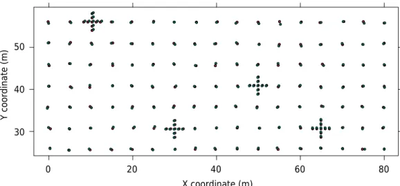
horizon-aligned grid and in the top 0.40 m soil layer in 0.02 m intervals. The spatial
to the original sampling scheme, drawing crosses over four randomly selected points
(Figure 1). In total, 151 vertical CI profiles were recorded with a cone (diameter 1.9 cm, apex angle 30°) (Asabe Standards, 2006) at each sampling time (before and after chiseling). To characterize the mean soil water content (SWC) of the study area, soil cores were extracted from a 0.00-0.40 m layer on a 10 × 10 m grid and SWC was estimated
by the gravimetric method for every 0.10 m interval.
Data analysis
The raw CI data (302 profiles) were pre-processed to eliminate systematic errors of soil
penetrometer measurements. The distribution of CI values was summarized per layer
using descriptive statistics and boxplots. Forty CI profiles were excluded prior to data
analysis because they contained observations that exceeded the three-fold interquartile
range from the first and third quartiles or were regarded as technical artifacts of the soil penetrometer measurements, such as reading failures. Data normality was assessed by the Shapiro-Wilks normality test per layer, and logarithmic transformation was performed
if needed. The spatial autocorrelation of CI readings was examined by computing sample variograms in horizontal and vertical directions. Because of the non-stationarity of CI along the vertical direction, a polynomial model was developed using soil depth as
explanatory variable. The trend coefficients were estimated by the generalized least squares (GLS) method and the sample variogram was computed using GLS residuals
(Webster and Oliver, 2007).
Bootstrap procedure
The estimators of the mean CI values per depth and their sampling distributions for
different sample sizes were obtained with a modified bootstrap procedure as follows:
1. One thousand bootstrap samples of size n were drawn with replacement from the
available CI profiles for each sampling time. The sample sizes ranged from 2 to 130
or 140, depending on whether the sampling time was before or after tillage. Because
of the spatial structure of CI along the vertical direction, each individual CI profile was regarded as resampling unit, so that the spatial autocorrelation was taken into account.
2. For each of the 1,000 bootstrap samples of a given size n, the vertical profiles of sample
median and mean of CI values were obtained by calculating these statistics per layer.
3. Finally, the estimators of the vertical profile of mean CI values and their standard error (SE) were calculated by computing the arithmetic mean and the standard deviation
of the bootstrapped sample median and mean of CI values of each layer.
Y coordinate (m)
50
40
30
X coordinate (m)
0 20 40 60 80
Figure 1. Sampling scheme of cone index (CI). Markers indicate sampling points before (filled
Determination of the minimum sample size
The minimum sample size to estimate the vertical profile of mean CI values with different levels of precision and confidence using the sample mean and median as estimators was determined by a procedure adapted from Dane et al. (1986) and Melo-Filho et al. (2002). The vertical profile of population mean CI values was estimated using the full data and the intervals were calculated with an error margin of ± 10, 20, 30, and 40 %. Then, the confidence level was calculated for each sample size (n) as the proportion (P) of vertical bootstrap profiles of the sample median and mean of CI values within a given
interval. Finally, the minimum sample size was determined by modeling the relation
between P and n using a locally-weighted polynomial function (LOESS) and obtaining the inverse predictions by a linear approximation function. Confidence levels of 0.95,
0.90, and 0.80 were used.
In addition, the minimum sample size was approximated by using the conventional
method based on the confidence interval of the mean (Equation 1). For each sampling
time, the variance of the process was estimated using the information from the most variable layer and the minimum sample size was calculated for the same level of precision
and confidence indicated above.
Data management and the bootstrap routine were carried out using the statistical
programming language R (R Core Team, 2017). Geostatistical analyses were performed
using the gstat package (Pebesma, 2004).
RESULTS AND DISCUSSION
Soil water contents at both sampling times were near field capacity and had low variation in the explored depth range; thus, no correction was applied to CI values (Table 1).
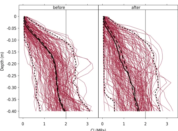
The variability in CI values was high at both sampling times and decreased with depth
(Figure 2). However, the sample CI profiles were more concentrated around the vertical profile of mean CI values before than after tillage (the average CV before and after tillage were 0.45 and 0.64, respectively). Before tillage, CVs >0.35 were observed from the surface to a depth of 0.20 m, whereas after tillage CV exceeded 0.35 in the entire depth range (Table 2). In general, the CVs reported in this study agree with those observed by
Alesso et al. (2017) in a similar soil under no-tillage, but are higher than those found by Özgöz et al. (2007) and Cavalcante et al. (2011), especially in the surface layers.
Before tillage, data from the 0.00 to 0.12 m depth range had right-skewed distributions, whereas after tillage, skewness was observed even to a depth of 0.20 m. However, according to the Shapiro-Wilks test, the distribution of CI values departed from normality only in the upper 7 and 13 layers before and after tillage, respectively. These results showed that surface layers are more variable and that due to the skewness of CI data, the
population mean of CI values in the surface layers would not be adequately estimated by
the sample mean. Similar results were reported by Gubiani et al. (2011), who concluded
that the sample mean represents CI values in compacted better than in chiseled soils,
due to the effect of tillage on soil structure. In this case, data transformation should be
applied to meet the assumptions, or a more robust estimator, such as the sample median, should be used instead of the sample mean. In this study, the logarithmic transformation did not approximate the CI data to a normal distribution. The sample mean and median
did not differ strongly due to the large sample sizes (Table 2 and Figure 2). However, larger differences between the vertical profiles of sample mean and median CI values
would be expected if the samples were smaller.
In the horizontal plane, the CI data showed no spatial structure at both sampling times,
thus each profile could be regarded as an independent sample unit. The lack of spatial
property was below the sampling scale due to the combination of small-scale variations
and measurement errors. In contrast, in the vertical direction (1D), CI showed a strong spatial structure (Figure 3). Similar results were reported by Castrignanò et al. (2002) on a Typic Chromoxerert from southern Italy and by Veronesi et al. (2012) on a Haplic Cambisol in the Czech Republic. In this study, the fitted global trend models before and
after tillage explained 40 and 57 % of the total variability of CI. In both cases, after
trend removal, a spherical model was fitted to the sample variogram and the estimated range showed differences as a result of tillage. Before tillage, the CI measurements
showed auto-correlation to a depth of 0.12 m whereas after tillage, this range of spatial dependence was extended to a depth of 0.16 m. The shorter range may be attributed to the layering produced by the continuous no-tillage system, inducing strong changes in the soil properties in deeper layers, whereas vertical tillage alters the soil structure by loosening the layers and extending the spatial continuity.
Sample size
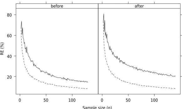
The relation between sample size and the maximum relative error (RE) of the sample median and mean of CI values approximated by bootstrap before and after tillage is
shown in figure 4. In general, the maximum RE of both estimators corresponds to the
Depth (m)
0
-0.05
-0.10
-0.15
Cl (MPa)
before after
-0.20
-0.25
-0.30
-0.35
-0.40
0 1 2 3 0 1 2 3
Figure 2. Spaghetti plots showing the variability of vertical profiles of cone index (CI) in MPa (gray lines) before and after tillage. Black lines represent the mean (solid line), median (dashed line),
and the 2.5th and 97.5th quantiles (dotted lines).
Table 1. Mean ± standard deviation of soil water content in 0.10-m intervals to a depth of 0.40 m, before and after tillage
Soil layer Before tillage After tillage
Soil water content
m g g-1
0.00-0.10 0.302 ± 0.017 0.271 ± 0.013
0.10-0.20 0.291 ± 0.012 0.279 ± 0.011
0.20-0.30 0.292 ± 0.015 0.280 ± 0.012
top 0.10 m of soil where the most variable CI readings were recorded. For both sampling times, the sample median of CI values showed higher RE compared to the sample mean over the entire range of sample size explored. In this study, the tillage increased the variability of CI readings resulting in higher RE of the sample mean or median of CI
values after tillage for a given sample size. Similar results were reported by Özgöz et al.
(2007) who concluded that all three tillage system evaluated (conventional, conservation,
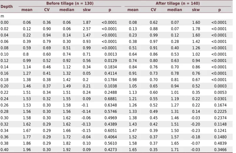
Table 2. Summary statistics of cone index (CI, MPa) recorded before and after tillage in 0.02-m intervals from the soil surface to the
maximum measured depth (0.40 m)
Depth Before tillage (n = 130) After tillage (n = 140)
mean CV median skw p mean CV median skw p
m
0.00 0.06 0.36 0.06 1.87 <0.0001 0.08 0.62 0.07 1.60 <0.0001
0.02 0.12 0.90 0.06 2.57 <0.0001 0.13 0.88 0.07 1.78 <0.0001
0.04 0.22 0.94 0.14 1.47 <0.0001 0.23 0.99 0.12 1.60 <0.0001
0.06 0.39 0.79 0.30 0.93 <0.0001 0.38 0.97 0.28 1.42 <0.0001
0.08 0.59 0.69 0.51 0.99 <0.0001 0.51 0.91 0.40 1.26 <0.0001
0.10 0.8 0.60 0.74 0.71 0.0013 0.64 0.86 0.53 1.02 <0.0001
0.12 0.99 0.52 0.92 0.56 0.0129 0.74 0.80 0.63 0.94 <0.0001
0.14 1.14 0.46 1.12 0.34 0.1834 0.84 0.76 0.70 0.86 <0.0001
0.16 1.27 0.41 1.32 0.05 0.4114 0.91 0.73 0.78 0.76 <0.0001
0.18 1.38 0.38 1.42 0.2 0.1784 0.98 0.70 0.81 0.67 <0.0001
0.20 1.46 0.37 1.49 0.21 0.1038 1.05 0.65 0.94 0.52 0.0003
0.22 1.51 0.34 1.51 0.24 0.2488 1.13 0.60 1.01 0.35 0.0053
0.24 1.53 0.32 1.55 0.09 0.6881 1.21 0.55 1.19 0.22 0.0301
0.26 1.53 0.30 1.58 -0.1 0.6348 1.26 0.52 1.27 0.22 0.1674
0.28 1.56 0.30 1.56 -0.14 0.5746 1.33 0.49 1.31 0.14 0.2225
0.30 1.58 0.30 1.62 -0.06 0.4969 1.38 0.45 1.46 -0.03 0.2374
0.32 1.62 0.29 1.62 -0.13 0.4389 1.43 0.42 1.51 -0.20 0.1148
0.34 1.67 0.29 1.66 -0.15 0.6051 1.47 0.39 1.50 -0.23 0.1241
0.36 1.77 0.29 1.72 -0.04 0.4064 1.52 0.37 1.57 -0.18 0.1480
0.38 1.86 0.29 1.82 0.10 0.5610 1.58 0.37 1.65 -0.07 0.4839
0.40 1.96 0.30 1.92 0.09 0.4273 1.65 0.35 1.71 -0.03 0.3466
CV: coefficient of variation; skw: skewness; and p: p-value of the Shapiro-Wilks normality test.
Cressie’s semivarianc
e
Distance (m) 0.30
0.25
0.20
0.15
0.10
0.05
0.05 0.10 0.15 0.20 0.25 0.05 0.10 0.15 0.20 0.25
before after
and reduced) increased variability of CI values. In addition, the RE associated with the sample median of CI values were greater than the RE of the sample mean because the
latter is a more efficient estimator, i.e. less variance. As a result, the number of samples
needed to achieve the same precision is also greater for the sample median. For example,
a maximum RE of 20 % around the vertical profile of sample mean CI values could be
expected with about 21 samples before tillage, whereas at least 24 observations are needed to achieve the same precision after tillage. In contrast, the same level of precision
around the vertical profile of sample median CI values could be achieved with about 66 observations before tillage, whereas more than 139 are needed after tillage.
The same general pattern of the relationship between sample size and error of the estimator was reported by Molin et al. (2012) and Tavares Filho and Ribon (2008) for Oxisols. However, in those studies the sample size above which no information is gained
by adding extra observations was significantly smaller than the results reported in figure 4. This could be explained by the differences of variability between soils and by the fact
that in those studies the CI data were collected or averaged per layer. The former study
reveals the soil-specific nature of the sample size recommendations, thus the greater the
soil variability, the higher are the sampling requirements. The latter article describes the
smoothing effect of sample support or data processing on the variability (Gubiani et al.,
2011), resulting in a smaller RE for the same sample size.
Although the approach described above is straightforward, it has a major drawback
by using only the information contained in the most variable soil layer and is based on the assumption of normality of the population being sampled. The alternative method proposed in this study is based on a resampling method and integrates the information
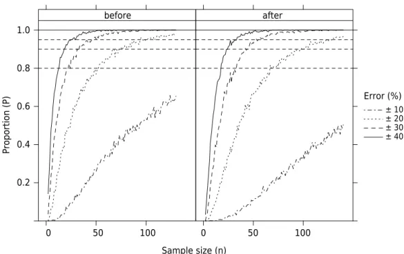
of the whole depth range down to 0.40 m, taking the vertical autocorrelation into account. The proportion of bootstrap vertical profiles of sample median and mean CI values falling within the intervals around the vertical profile of the population of mean
CI values increases with the sample size for all error margin levels, as expected for both estimators (Figure 5). However, for the sample median, none of the curves reached the
line P = 1, neither before nor after tillage. In contrast, for the sample mean, the curves ± 20, 30, and 40 % reached the plateau level within the available maximum sample size (n = 130 and 140) although the sampling sizes were always greater after tillage
RE (%)
80
60
40
20
0 50 100
Sample size (n)
0 50 100
before after
Figure 4. Relation between sample size (n) and the maximum relative error (RE) of the vertical
profile of mean (solid line) and median (dashed line) cone index (CI) values approximated by
(Figure 6). These results show that the sampling distribution of the sample median was
more variable than that of the sample mean. Also, they show the effect of soil tillage on
soil variability because the relationship between sample size and proportion of bootstrap
profiles within confidence intervals tended to be less steep after soil tillage.
In general, the number of sample profiles required for the estimation of the vertical profile
of mean CI values increased with the variability of CI readings and the desired level of
precision and confidence (Table 3). The higher variability of CI observed after tillage resulted in greater sampling requirements for all levels of precision and confidence,
Proportion (P
)
1.0
0.8
0.6
0.4
0.2
Sample size (n)
Error (%)
before after
± 10
0 50 100 0 50 100
± 20 ± 30 ± 40
Figure 5. Proportion of bootstrap vertical profiles of sample median of cone index (CI) values that fall within the ± 10, 20, 30, and 40 % of error around the vertical profile of mean CI values,
before and after tillage.
Proportion (P
)
1.0
0.8
0.6
0.4
0.2
Sample size (n)
Error (%)
before after
± 10
0 50 100 0 50 100
± 20 ± 30 ± 40
Figure 6. Proportion of bootstrap vertical profiles of sample mean of cone index (CI) values that fall within the ± 10, 20, 30, and 40 % of error around the vertical profile of mean CI values, before
independent of the estimator being used. In addition, at the same level of variability of
CI readings, precision and confidence, the sampling requirements are higher when the profile of mean CI values is estimated by the sample medians. For example, to estimate the profile of mean CI values with an error of less than 20 % and a confidence level of 90 %, it would be necessary to take more than 129 and 139 sample profiles before and
after tillage, respectively. In contrast, if the estimators were the sample means, the
sampling requirements would drop to 74 and 97 sample profiles of CI before and after
tillage, respectively. Estimating sampling needs with the conventional method, which assumes normal distribution of the CI data and is based solely on the information of the most variable layer, resulted in smaller sampling sizes. For instance, for the same level
of precision and confidence, 64 and 81 sample profiles would be required before and
after tillage, respectively, according to this method. This discrepancy between methods suggests that bootstrapping is a more robust method to assess true population variation
based on information of the entire profile.
In all cases, the estimated sample sizes (Table 3) exceeded the sampling recommendations reported in other studies (Tavares Filho and Ribon, 2008; Molin et al., 2012; Storck et al., 2016).
For example, the general recommendation of 20 samples would result in an estimation of the
vertical profile of mean CI values with an error near ± 40 %, the 80 % of the times at best,
independently of the estimator or the sampling time. Nevertheless, the precision achieved with 15-20 samples is below than the 10 % threshold suggested by the above authors.
The bootstrap method can be used without requiring knowledge of the distribution of
the sampling population, whereas the conventional sample size determination method
depends on knowledge or assumptions about the distribution (Dane et al., 1986). Moreover,
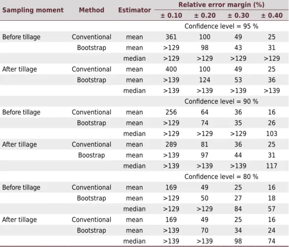
Table 3. Minimum sample sizes needed to estimate the vertical profile of mean cone index (CI) values with different levels of precision and confidence before and after soil tillage determined by conventional and bootstrap methods, using the vertical profile of sample mean and median
values as estimators
Sampling moment Method Estimator Relative error margin (%)
± 0.10 ± 0.20 ± 0.30 ± 0.40
Confidence level = 95 %
Before tillage Conventional mean 361 100 49 25
Bootstrap mean >129 98 43 31
median >129 >129 >129 >129
After tillage Conventional mean 400 100 49 25
Bootstrap mean >139 124 53 36
median >139 >139 >139 >139
Confidence level = 90 %
Before tillage Conventional mean 256 64 36 16
Bootstrap mean >129 74 35 26
median >129 >129 >129 103
After tillage Conventional mean 289 81 36 25
Boostrap mean >139 97 44 31
median >139 >139 >139 117
Confidence level = 80 %
Before tillage Conventional mean 169 49 25 16
Bootstrap mean >129 50 27 18
median >129 >129 84 57
After tillage Conventional mean 169 49 25 16
Bootstrap mean >139 70 34 24
it is readily understood and easy to use, provided the assumptions are met, but depends strongly on how well the variance of the process is approximated (Han et al., 2016). On the other hand, bootstrapping methods are conceptually more complex and require computer software to perform the simulations, but are superior to the parametric methods, for capturing the variability more precisely and estimating the sampling distribution without assumptions. These features allow researchers to deal with distributions other than normal, as is common for soil properties. In particular, the method outlined here considers the
vertical autocorrelation by performing the resampling procedure at the soil profile level.
CONCLUSIONS
The proposed bootstrap approach allows the approximation of the sampling distribution
of the vertical profiles of soil cone index and the determination of the sample size required for the estimation of a vertical profile of mean CI values using different estimators and levels of precision and confidence. Unlike the conventional method,
the proposed approach did not assume any theoretical distribution and uses the
information of the whole soil profile including the vertical autocorrelation of CI
readings, which is a great advantage.
Results of this study demonstrate that the bootstrap approach may be used to determine
the implications of soil variability on the sampling efforts required for an accurate estimation of soil resistance in soils subjected to different soil management practices. However, more research is needed to explore the effect of different soil types, tillage
practices, and penetrometers on the sample needs.
ACKNOWLEDGEMENTS
The authors are grateful to the Facultad de Ciencias Agrarias, Universidad Nacional del Litoral through (Esperanza, Argentina), and Consejo Nacional de Investigaciones
Científicas y Técnicas (CONICET, Santa Fe, Argentina) for financial and operational support of this research by the grant PIP No. 677/Res. D5202. The assistance of Mr. Masola and undergraduate students at UNL-FCA is gratefully acknowledged.
REFERENCES
Alesso CA, Carrizo ME, Imhoff SC. Mapping soil compaction using indicator kriging in Santa Fe province, Argentina. Acta Agron. 2017;66:81-7. https://doi.org/10.15446/acag.v66n1.54775 Asabe Standards. ASAE S313.3: Soil cone penetrometer. St. Joseph: American Society of Agricultural & Biological Engineers; 2006.
Castrignanò A, Maiorana M, Fornaro F, Lopez N. 3D spatial variability of soil strength and its change over time in a durum wheat field in Southern Italy. Soil Till Res. 2002;65:95-108. https://doi.org/10.1016/S0167-1987(01)00288-4
Cavalcante EGS, Alves MC, Souza ZM, Pereira GT. Variabilidade espacial de atributos físicos do solo sob diferentes usos e manejos. Rev Bras Eng Agric Ambient. 2011;15:237-43. https://doi.org/10.1590/S1415-43662011000300003
Chernick MR. Bootstrap methods: a guide for practitioners and researchers. 2nd ed. New Jersey: Wiley-Interscience; 2008.
Gubiani PI, Reichert JM, Reinert DJ, Gelain NS. Implications of the variability in soil penetration resistance for statistical analysis. Rev Bras Cienc Solo. 2011;35:1491-8. https://doi.org/10.1590/S0100-06832011000500003
Han Y, Zhang J, Mattson KG, Zhang W, Weber TA. Sample sizes to control error estimates in determining soil bulk density in California forest soils. Soil Sci Soc Am J. 2016;80:756-64. https://doi.org/10.2136/sssaj2015.12.0422
Instituto Nacional de Tecnología Agropecuaria - INTA. Carta de suelos de la República Argentina: Hojas 3160 - 26 y 25 Esperanza-Pilar. Rafaela: INTA EEA; 1991.
Letey J. Relationship between soil physical properties and crop production. Adv Soil S. 1985;1:277-94. https://doi.org/10.1007/978-1-4612-5046-3_8
McBratney AB, Webster R. How many observations are needed for regional estimation of soil properties? Soil Sci. 1983;135:177-83.
Melo-Filho JF, Libardi PL, Jong Van Lier Q, Corrente JE. Método convencional e “bootstrap” para estimar o número de observações na determinação dos parâmetros da função Ks. Rev Bras Cienc Solo. 2002;26:895-903. https://doi.org/10.1590/S0100-06832002000400006
Molin JP, Dias CTS, Carbonera L. Estudos com penetrometria: novos equipamentos e amostragem correta. Rev Bras Eng Agric Ambient. 2012;16:584-90.
https://doi.org/10.1590/S1415-43662012000500015
Mulla DJ, McBratney AB. Soil spatial variability. In: Sumner ME, editor. Handbook of soil science. Boca Raton: CRC Press; 2000. p.A-321-52.
Özgöz E, Akbaş F, Çetin M, Erşahin S, Günal H. Spatial variability of soil physical properties as affected by different tillage systems. New Zeal J Crop Hort. 2007;35:1-13. https://doi.org/10.1080/01140670709510162
Pebesma EJ. Multivariable geostatistics in S: the gstat package. Comput Geosci. 2004;30:683-91. https://doi.org/10.1016/j.cageo.2004.03.012
R Core Team. R: a language and environment for statistical computing. Vienna: R Foundation for Statistical Computing; 2017.
Rooney DJ, Lowery B. A profile cone penetrometer for mapping soil horizons. Soil Sci Soc Am J. 2000;64:2136-9. https://doi.org/10.2136/sssaj2000.6462136x
Sokal RR, Rohlf FJ. Biometry: the principles and practice of statistics in biological research. 4th ed. New York: WH Freeman; 2012.
Storck L, Kobata SGK, Brum B, Soares AB, Modolo AJ, Assmann TS. Sampling plan for using a motorized penetrometer in soil compaction evaluation. Rev Bras Eng Agríc Ambient. 2016;20:250-5. https://doi.org/10.1590/1807-1929/agriambi.v20n3p250-255
Tavares Filho J, Ribon AA. Resistência do solo à penetração em resposta ao número de amostras e tipo de amostragem. Rev Bras Cienc Solo. 2008;32:487-94. https://doi.org/10.1590/S0100-06832008000200003
Usowicz B, Lipiec J. Spatial distribution of soil penetration resistance as affected by soil compaction: the fractal approach. Ecol Complex. 2009;6:263-71. https://doi.org/10.1016/j.ecocom.2009.05.005 Veronese Júnior V, Carvalho MP, Dafonte J, Freddi OS, Vidal Vázquez E, Ingaramo OE. Spatial variability of soil water content and mechanical resistance of Brazilian ferralsol. Soil Till Res. 2006;85:166-77. https://doi.org/10.1016/j.still.2005.01.018
Veronesi F, Corstanje R, Mayr T. Mapping soil compaction in 3D with depth functions. Soil Till Res. 2012;124:111-8. https://doi.org/10.1016/j.still.2012.05.009
Wang JF, Stein A, Gao BB, Ge Y. A review of spatial sampling. Spat Stat-Neth. 2012;2:1-14. https://doi.org/10.1016/j.spasta.2012.08.001
Warrick AW, Van Es HM. Soil sampling and statistical procedures. In: Dane JH, Topp CG, editors. Methods of soil analysis: Physical methods. 3rd ed. Madison: Soil Science Society of America; 2002. Pt.4. p.1-200.