Barrier option pricing via heston model

(1)

BARRIER OPTION PRICING VIA HESTON MODEL

Igor Kravchenko

A Thesis submitted for the degree

of Master of Finance

Thesis Supervisor:

Prof. João Pedro Nunes, Professor, ISCTE Business School, Department of Finance

(2)

Resumo

O objectivo desta tese é analisar a avaliação de opções de barreira no modelo de [Heston, S.L. (1993)]. Seguindo a abordagem presente em [Griebsch, S.A., and Pilz, K.F. (2012)] é estabelecido um preço para as opções de compra up-and-out via modelo de [Heston, S.L. (1993)]. Vários tópicos introdutórios são incluídos para evidenciar as semelhanças no método e nas técnicas aplicadas. A implementação numérica é feita em Matlab. O preço da opção barriera é calculado através de três métodos diferentes no caso mais simples. Para o caso geral, o algoritmo foi desenvolvido e implementado mas não produziu resultados satisfatórios.

Palavras-Chave: Modelo de Heston, opções barreira, transformada rápida de

(3)

Abstract

The thesis objective is to analyse the valuation of barrier options in the [He-ston, S.L. (1993)] model. Following [Griebsch, S.A., and Pilz, K.F. (2012)] approach up-and-out calls are priced via Heston model. Several introductory topics are included to evidence the similarities in the method and the tech-niques applied. The numerical implementation is done in Matlab. The price for the option is calculated through three di¤erent methods in a simplest case. For the general case, the algorithm was developed and implemented but it did not present satisfactory results.

(4)

1 Introduction

Today, in the middle of the European debt crisis, the theme of complex …nan-cial instruments became an everyday public discussion. The fast developed option pricing methods, started with [Black, F., and Scholes, M. (1973)] model, have grown into complicated structures and became an inseparable part of the market. In this paradigm, the e¢ cient price calculation techniques are highly valued. It is important to understand the di¢ culties presented by these instruments on both theoretical and implementation levels. Here, we will center our attention on the price calculation of one particular exotic option, the barrier option.

[Heston, S.L. (1993)] o¤ers a closed form solution for the pricing of European-style standard options with stochastic volatility. The resulting model became quickly popular amongst the practitioners. In this thesis, mostly based on [Griebsch, S.A., and Pilz, K.F. (2012)], we look at the pric-ing of European-style barrier options under the [Heston, S.L. (1993)] model.

The thesis has the following structure.

Chapter 1 introduces the general concepts of the stochastic calculus and the Black-Sholes market model in particular. We focus in more detail on the …rst hitting time distribution, since it plays an important role in our approach to the pricing of barrier options. In the context of the Black-Sholes model we review how the barrier options are treated and what di¢ culties they present.

(8)

Chapter 2 presents the [Heston, S.L. (1993)] model and, in particular, the famous [Heston, S.L. (1993)] formula for standard call options.

Chapter 3 is dedicated to our main problem: to …nd the valuation for-mula for up-and-out calls under the [Heston, S.L. (1993)] model. We start by conditioning the options pay-o¤ on variance paths and calculating the resulting joint distribution of the maximum to date and the generator of the process. The problem is analysed in three cases, because the model para-meters in‡uence the di¢ culty of the task. In the …rst case, we assume that there is no correlation between the two generator processes involved and the risk free rate is equal to the dividend yield. In the second case, we only maintain the zero correlation assumption and in the third case we study the general situation with no restrictions on the parameters. Next, we proceed to unconditioning. We analyse in detail only the cases 1 and 3. We derive the exact formula for the up-and-out call in the case 1 and an approximated one for the general case 3.

Finally, Chapter 4, is dedicated to the numerical analysis and to imple-mentation issues. We describe some of the techniques used and develop the algorithms for the cases 1 and 3. The numerical tool used was Matlab. We compare the results obtained by the algorithms presented in the Appendix of the thesis.

(9)

1.1 Barrier options

The barrier option (BO) is a path dependent option which becomes either active or extinguished when the underlying asset reaches the “barrier”level. To illustrate this options a little better, we will de…ne an European-style up-and-out call.

The European up-and-out call is an option to buy a certain asset S, at a strike price K and at a time T , if the price of the asset never reaches the barrier B until time T . The …nal pay-o¤ of this option is

VT = 8 > < > : (ST K)+ if sup 0 t T St< B 0 otherwise (1.1)

The previous de…nition includes the following concepts:

European - the option that can only be exercised at the speci…c time T . Other possibilities could be Bermudian (can be exercised on several pre-chosen dates), American (can be exercised at any time), Asian (average price for a pre-chosen period of time), etc.

Up - referring to an upper barrier B. Other possibilities would be down (down barrier) or both barriers (double barrier).

Out - the BO becomes extinct when touching a barrier. Other pos-sibility would be “in”, if option is activated only upon reaching the barrier.

(10)

Call - the option to buy an asset S, at a strike price K. Other possibility would be a put option, i.e. the right to sell an asset S, at a strike price K.

1.2 General assumptions

For the purpose of this thesis, we will consider certain theoretical assumptions regarding the market-trading universe, which are considered to be standard. We try to look at them from a BO point of view:

Every variable has a continuos path, in particular the asset price S. In practice, of course, this is not true. Even if we consider a basis point to be our approximation to continuity, during times of “big news”, market jumps are far from basis point ticks. An important consequence of the continuity assumption is that the probability of any particular price Sp

(or Sp = B) is zero; hence, we can only work with intervals.

The market is unique and liquid enough for any transactions, so in our model we know without ambiguity when the barrier is triggered. In practice these matters have to be carefully de…ned in the contract, namely: underlying asset, underlying market or markets, private or public trades, volume of the trade necessary to be considered a barrier breach, etc.

(11)

1.3 Brownian motion and the Black-Scholes model

With the previous assumptions in mind, we can start to develop a model for the market and later calculate the price for BOs. As ground work to obtain the price for BOs via [Heston, S.L. (1993)] model, we analyse the derivation via the simpler [Black, F., and Scholes, M. (1973)] model …rst. This will allow us to de…ne some necessary notions and correspondent useful results. For this part we have [Shreve, S.E. (2000)] as our main reference.

1.3.1 First passage time distribution

De…nition 1 (Brownian Motion) _{Consider a probability space ( ; F; P).} For each ! 2 , the continuous function W (t), t 0, that satis…es W (0) = 0, depends on ! and for all t0 < t1 < ::: < tn the increments

W (t1) = W (t1) W (t0); W (t2) W (t1); :::; W (tn) W (tn 1)

are independent and normally distributed with: E[W (ti+1) W (ti)] = 0

V ar[W (ti+1) W (ti)] = ti+1 ti

is called Brownian Motion (BM). [Shreve, S.E. (2000)] De…nition 3.3.1. The BM is the center of the stochastic calculus, developed …rst in physics to deal with the randomness of particle movements. One of the main concepts is the “di¤erentiation” of the function whose variable is a BM (or more generally a stochastic process) through the Ito’s Lemma, which is stated in the Appendix as Theorem 1.

(12)

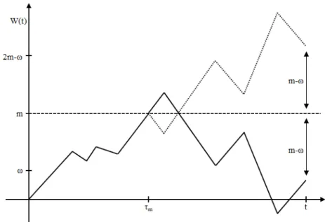
Figure 1.1: Illustration of Re‡ection Principle

The First passage time and maximum distributions

We start by deriving the distribution for the …rst passage time. Consider

m - the …rst passage time through level m for BM W (t).

The Figure 1.1 illustrates the path of W (t) and its re‡ected path f

W (t) = W m^t (Wt W m^t); using the notation a ^ b = inf(a; b).

The BM is symmetrical with respect to the time axis. We know that the path of W (t) crosses level m at m t. For every path that ends

(13)

2m ! = ((m !) + m). This observation gives us the Re‡ection Principle, [Shreve, S.E. (2000)] Theorem 3.7.1.

P( m t; W (t) !) = P(W (t) 2m !): (1.2)

We can use equation (1.2) to calculate the distribution of the …rst passage time . With choice ! = m and assuming m > 0, equation (1.2) becomes:

P( m t; W (t) m) = P(W (t) m):

On the other hand, it is always true that:

P( m t; W (t) m) = P(W (t) m):

Combining both equations:

P( m t) = 2P(W (t) m) = 2 p 2 t 1 Z m e x22tdx;

since, W (t) has normal distribution with E[W (t)] = 0 and V ar[W (t)] = t. Next, we introduce the concept of Maximum to Date:

M (t) = sup

0 s t

W (s): (1.3)

We can rewrite the re‡ection principle (1.2) as:

P(M(t) m; W (t) _{!) = P(W (t)} 2m !); ! m; m > 0: (1.4) From equation (1.4) we can obtain the joint density distribution of (M (t); W (t)), i.e. f(M (t);W (t)) di¤erentiating twice, …rst in order to m and then in order to

!: 1 Z m ! Z 1 f(M (t);W (t))(x; y)dxdy = 1 p 2 t 1 Z 2m ! e z22tdz f(M (t);W (t))(m; !) = 2(2m !) tp2 t e (2m !)2 2t ; (1.5)

(14)

see [Shreve, S.E. (2000)] Theorem 3.7.3. Consider the BM with a drift constant

^

W (t) = t + W (t); 0 t T;

where W (t) is a BM that has zero drift (i.e. it is a martingale) under the orig-inal measure P, de…ned on a probability space ( ; F; P). We de…ne maximum to date for ^W as ^ M (t) = sup 0 s t ^ W (s): (1.6)

To calculate the joint density distribution of ( ^M (T ); ^W (T )) it is necessary to know how to change measures.

Theorem 2 (Girsanov, one-dimension) Let W (t); 0 t T; be a BM on ( ; F; P), and F(t) be a …ltration for this BM. Let (t), 0 t T, be an adapted process. De…ne

Z(t) = exp_f t Z 0 (u)dW (u) 1 2 t Z 0 2_(u)du g; f W (t) = W (t) + t Z 0 (u)du;

and assume that

E[ T Z 0 2_(u)Z2_{(u)du] <} 1

Set Z = Z(T ). Then EZ = 1 and under the probability measure eP given by eP =Z

A

Z(!)dP (!) for all A_{2 F;}

(15)

Proof. For a proof see, for instance, [Shreve, S.E. (2000)] Theorem 5.2.3 or [Øksendal, B. (2002)] Theorem 8.6.3

With the help of Girsanov theorem and equation (1.5) we can calculate the joint density distribution of ( ^M (T ); ^W (T )) as

f_{( ^}_{M (T ); ^}_{W (T ))}(m; !) = 2(2m !) Tp2 T e ! 1 2 2_T 1 2T(2m !) 2 ; ! m; m 0; (1.7) or zero for other values of m and !, see [Shreve, S.E. (2000)] Theorem 7.2.1.

1.3.2 The Black and Scholes (1973) model

The Black-Sholes (BS) …nancial market model created a revolution in option pricing and, consequently, in option trading. It o¤ered a clear pricing method for European-style standard options, making the option trading more trans-parent and understandable. In the BS model, the asset price S(t) follows a geometric BM. The associated stochastic di¤erential equation (SDE) under the physical measure P is

dS = Sdt + SdWS; (1.8)

where is the drift or expected rate return of the asset, is the standard deviation of the rate of return on the asset, and WS _{is a standard BM. We}

can rewrite equation 1.8 using Girsanov theorem 2 with = (r q), where r is the risk free rate and q is dividend yield we arrive at Black-Scholes-Merton equation [Merton, R (1973)]:

(16)

where fW _{is a standard BM under the risk neutral measure Q. The solution} for the SDE (1.9) is

S = S0e fW +((r q)

1

2 2)t: (1.10)

Using Ito’s Lemma, from the Theorem 1 in Appendix for an option V (t; S) we derive:1 dV = Vtdt + VSdS + 1 2VSS 2_S2_dt = (Vt+ (r q)SVS+ 1 2 2_S2_V SS)dt + VS SdfW ; (1.11)

Since e_E[VS SdfWjF(t)] = 0, then

e E[dV jF(t)] = (Vt+ (r q)SVS + 1 2 2_S2_V SS)dt: (1.12)

On the other hand, under (1.12) the risk neutral measure e

E[dV jF(t)] = rV dt: (1.13)

Joining equations (1.12) and (1.13), we derive the Black-Scholes-Merton par-tial di¤erenpar-tial equation (PDE):

Vt+ (r q)SVS +

1 2

2_S2_V

SS = rV: (1.14)

1.3.3 Barrier options under Black-Scholes model

Here we follow [Shreve, S.E. (2000)], chapter 7. 1_{Here the subscript indicates the derivative} @V

(17)

Proposition 3 The price of an up-and-out call at time t, satis…es the PDE equation (1.14) and the boundary conditions

V (t; 0) = 0; 0 t T;

V (t; B) = 0; 0 t T;

and

V (T; S) = (S(t) K)+; 0 S(t) < B; assuming that the option was not knock-out before time t.

We will not proof Proposition 3 directly (i.e. solve the Cauchy problem) but we can verify it later. Instead, we will calculate the price of an up-and-out call by the direct application of the re‡ection principle.

The pay-o¤ of the up-and-out call is given by equation (1.1). Since S(t) is given by equation (1.10), de…ning ^M (T ) as in (1.6) and

^ W (T ) = fW (T ) + r q 2 2 _T; we have: V (T ) = 8 < : (S(T ) K)+ _{= (S(0)e} W (T )^ _{K) if} _{M (T ) < b}_^ 0 if M (T )^ b ; with b = 1log(_S(0)B ), or V (T ) = (S(0)e W (T )^ K)+[1_M^_T_<b] = (S(0)e W (T )^ K)[1_W^_T_{>k; ^}_M_T_<b];

(18)

with k = 1 log(_S(0)K ). Hence, V (0) = b Z k b Z !+ e rT(S(0)e w K)f_{( ^}_{M (T ); ^}_{W (T ))}(m; w)dmdw:

with !+ _{= sup(!; 0). Using the density distribution of ( ^}_{M (T ); ^}_{W (T ))} _given

by equation (1.7), with = r q 2 2 _; then V (0) = b Z k b Z !+ e rT(S(0)e ! K)2(2m !) Tp2 T e ! 1₂ 2T _2T1 (2m !)2_dmd! = b Z k (S(0)e ! K)_p1 2 Te rT + ! 1₂ 2_T 1 2T(2m !) 2 m=b m=!+ d! = S(0)I1 KI2+ S(0)I3 KI4; (1.15)

where Ij is the representation for the four integrals contained in equation

1.15, each of them is of the form 1 p 2 T b Z k e + ! 21 ! 2 dw = e12 2_{T +} [_{N (}b_p T T ) N ( k T p T )]; (1.16) for some and . Introducing

( ; s) = _p1

t[log s + (r 1 2

(19)

and using equation (1.16), Ij can be solved as I1 = N ( +(T; S(0) K )) N ( +(T; S(0) B )) I2 = e rT[N ( (T; S(0) K )) N ( (T; S(0) B ))] I3 = ( S(0) B ) 2r 2 1₍_{N (} +(T; B2 KS(0))) N ( +(T; B S(0))) I4 = e rT( S(0) B ) 2r 2+1₍_{N ( (T;} B 2 KS(0))) N ( (T; B S(0))):

We can check that under the assumptions T > t, 0 S(0) = S B, our so-lution veri…es the Black-Sholes-Merton PDE (1.14) with boundary conditions given by Proposition 3.

2 Heston (1993) model

2.1 Introduction

The stochastic volatility model, given by the equations

dSt = (r q)Sdt +pvtSdWtS; (2.1)

dvt = ( vt)dt + pvtdWtv; (2.2)

and

dW_tSdW_tv = dt: (2.3)

is known as the Heston (1993) model. The typical introduction of any volatil-ity model starts with the explanation of the limitations of the BS model.

(20)

One randomness source is simply not enough. Hence, to satisfy the customer (market), we need to introduce another element of randomness: the stochas-tic process for the variance given by equation (2.2)2. The goal is to make the new model “smile” on the volatility axis, in opposition to the rigid ‡at volatility from the BS model. The third equation establishes the correlation between the two BM’s. The processes involved are: the spot price process St,

the instantaneous volatility vt of logarithmic spot price with initial variance

v0 …xed and the standard BM’s WtS and Wtv. Model parameters are: the

dividend yield q, the risk free rate r, the mean reversion speed of variance , the mean reversion level for the variance , the volatility of the variance and the correlation between two BM’s. To ensure the strictly positive volatility we have to enforce the Feller condition on the parameters

2 > 2:

See, for instance, [Karatzas, I., and Shreve, S. (1991)].

Since the model has two BM’s (random sources) and only one tradable asset St, our market model is incomplete. To complete it, we should have

introduced another tradable asset, like an European call, for example. See [Hull, J. C., and White A. (1987)].

2_{The stochastic equation is known as a CIR (Cox, Ingersoll and Ross) process, see [Cox,}

(21)

2.2 Standard European call option price

The call price at time t under risk neutral measure Q is given by ct(S; K; T ) = e r EQ[(ST K)+]:

where = T t is the time to expiration and K is the strike price, i.e.: ct(S; K; T ) = e r EQ[ST1ST>K] e

r

KEQ[1ST>K]: (2.4) Introducing the logarithmic spot price

xt= log St; (2.5)

the probability of the call expiring in-the-money under risk neutral measure Q is the second term in equation (2.4):

EQ[1ST>K] = Q(ST > K) = Q(log ST > log K) = P2(x; v; ): (2.6) The …rst term in equation (2.4) needs a measure change due to ST term. We

introduce the Radon-Nykodim derivative (see [Shreve, S.E. (2000)]) by Zt =

Steqt

STeqT

er ; and de…ne the probability measure

Qs=

Z

A

er _ZtdQ for all A 2 F(t):

The …rst term on the right-hand side of equation (2.4) becomes e r _EQ[ST1ST>K] = E Q_[e r ST1ST>K] = EQs_[e r _S T1ST>KZt] = Ste q EQs[1ST>K] = ext q Qs(ST > K) = ext q P1(x; v; ): (2.7)

(22)

Considering equations (2.4), (2.6) and (2.7), then

ct(S; K; T ) = ext q P1(x; v; ) e r KP2(x; v; ) (2.8)

We can express the solution (2.8) through the characteristic function of xt,

method used in [Heston, S.L. (1993)]. Later on, we will use the same tech-nique in our barrier option calculations and show it in more detail, so here, we will announce the idea and present the solution from [Heston, S.L. (1993)]. The both probabilities Pj have to satisfy the Heston PDE

Vt+ 1 2vS 2_V SS+ vSVvS + 1 2 2_vV vv rV + (r q)SVS+ ( v)Vv = 0:

We use the Feynman-Kac theorem described in the Appendix 5.2 to calculate the characteristic functions

fj(x; v; T ; u) = EQj[exp(iuxT)jFt];

with Q1 = Qs and Q2 = Q, using the guess

fj(x; v; T ; u) = exp(Cj( ; u) + Dj( ; u)v + iux)

and obtaining the probabilities Pj through the Inversion Theorem 4 by

Pj = 1 2+ 1Z1 0 Re[e iu log K_f j(x; v; u) iu ]du:

The solution for j = 1; 2 is

Cj = (r q)iu + ₂[(bj iu + dj) 2 log( 1 gjedj 1 gj )] Dj = bj iu + dj 2 ( 1 edj 1 gjedj );

(23)

with gj = bj iu + dj bj iu dj dj = q ( iu bj)2 2(2ljiu u2) b1 = b2 = lj = ( 1)1+j 1 2

3 Barrier options via Heston (1993) model

Our objective is to compute the price of an up-and-out call assuming that the market is described by the Heston (1993) model. As in the case of the standard European call, a closed form solution is not known. Hence, we will use the same technique: to represent the solution in an integral form through the characteristic function. We will follow [Griebsch, S.A., and Pilz, K.F. (2012)], starting by the conditioning of the option expected payo¤ on variance paths, eliminating this way one source of randomness. Afterwords, we can calculate the arising conditioned expectation in closed form. At the end, we resolve the conditioning.

(24)

3.1 Conditioning on variance paths

The payo¤ of an up-and-out option is given by (1.1), and its discounted payo¤ is

V0 = e rTEQ[VTjF0]

where, Ft is the …ltration associated with BM’s Ws and Wv, or simply, F0

are initial conditions. We want to condition on a -algebra generated by variance paths up to time T , i.e.

GTv = (fvs : 0 s Tg): (3.1)

The conditioning on the variance paths will eliminate one source of random-ness from the model. The tower property of conditional expectations and the payo¤ formula gives us3

V0 = e rTE[E[VTjGTv]jF0] = e rT_E[E[(ST K)+If sup 0 t T St<BgjG v T]jF0]:

Introducing the notation

Ev=E[(ST K)+If sup 0 t T St<BgjG v T]; (3.2) we rewrite V0 = e rTE[EvjF0]:

(25)

Applying Ito’s lemma to xt, logarithmic spot price, given by (2.5) we have: dxt = @ log S @t dt + @ log S @S dS 1 2 @2_{log S} @S2 dSdS = 0dt + 1 SdS 1 2 1 S2dSdS = (r q)dt +pvdWS 1 2vdt; or in integral form xt = x0+ (r q)t + t Z 0 p vdW_sS 1 2 t Z 0 vsds: (3.3)

We proceed by using the information from equations (2.2) and (2.3). Since WS _{and W}v _{are correlated, we want to isolate W}v _{for more e¤ective}

condi-tioning. Please consider the Cholesky decomposition A = L L where L is a lower triangular matrix and L is its conjugate transpose:

L = 2 41 _p 0 1 2 3 5 L L = 2 41 1 3 5 :

Hence, there is an independent BM W that satis…es dWS = dWv+p1 2_dW:

Then, equation (3.3) becomes

xt = x0+ (r q)t 1 2 t Z 0 vsds + t Z 0 p_v sdWsv+ 2 t Z 0 p_v sdWs; (3.4)

(26)

where 2 =

p

1 2_{. The second equation of the model in the integral form}

is vt = v0+ t t Z 0 vsds + t Z 0 p vsdWsv: Isolating the t R 0 p vdWv

s term and inserting it in the equation (3.4), we obtain:

xt= x0+(r q)t 1 2 t Z 0 vsds+ (vt v0 t+ t Z 0 vsds)+ 2 t Z 0 p vsdWs: (3.5)

Using the abbreviation

(t) = (r q)t 1 2 t Z 0 vsds + (vt v0 t + t Z 0 vsds); equation (3.5) becomes xt = x0+ (t) + 2 t Z 0 p vsdWs:

Logarithmic spot price is the sum of: its initial value, a time-dependent drift (t) and an Itô integral 2

t

R

0

p_v

sdWs. Now the conditioning on the variance

paths (Gv

t de…ned in (3.1)) looks appealing and a new variable4

xv_t = xtjGtv;

has a single random contribution, which arises from

Yt = 2 t Z 0 p vsdWs;

4_{Further, we will use the superscript v to identify variables subjected to conditioning}

(27)

The variable vt cannot be negative. The variable Ythas normal distribution, because in Gv t, vt is non-random, i.e. Yt N (0; 22 2(t)); where 2_{(t) =} t Z 0 vsds: The variable xv

t is also normally distributed

xv_t _{N (} v(t); 2₂ 2(t)); with mean

v_{(t) = x}

0+ v(t):

Note that v_(t) _{is a deterministic continuos function, but nowhere}

di¤eren-tiable (due to vs term), unless = 0.

Next objective is to rewrite the equation (3.2) for Ev, through the new variables

^

Yt = (t) + Yt

^

Mt = supf ^Ys: 0 s tg;

and using the observations

xt= log St= x0+ ^Yt; St= ex0e ^ Yt _{= S} 0e ^ Yt_; sup St < B =) sup S0e ^ Yt _{< B =} ) ^Mt< b = log( B S0 );

(28)

ST K > 0 =) ^YT > k = log( K S0 ); we can rewrite (3.2) as Ev = E[(S0e ^ Yt K)If ^Mt<b; ^Yt>kgjG v T] = Ev[(S0e ^ Yt K)If ^Mt<b; ^Yt>kg]: (3.6) To calculate the expectation Ev _{we need the joint distribution of ( ^}_{Y ; ^}_{M )}

under the probability measure Qv_.

3.1.1 Derivation of the joint density distribution for

(M (T ); Y (T ))

Proposition 1 (Re‡ection Principle) _{Let fY}tgt 0be an Itô process of the

form Yt= t Z 0 (s)dWs (3.7)

with deterministic and Mt = sups tYs for t 0. Then the re‡ection

principle holds,

Q(Mt x; Yt < y) = Q(Yt> 2x y) f or all t 0; x y_ 0:

Therefore,

Qv(Mt x; Yt y) = Qv(Yt 2x y): (3.8)

Proof. For a proof see [Griebsch, S.A., and Pilz, K.F. (2012)], theorem 1.

We can use the previous proposition to calculate the density distribution of (M (T ); Y (T )). Consider Yt de…ned by (3.7). Then,

(29)

Proposition 2 _{For m 6= 0 the random variable} m = infft 0 : Yt mg

has the following distribution

Qv(Mt m) = Qv( m t) = 2 p 2 +1 Z jmj p2 2 2(t) e 12y 2 dy:

Proof. Following [Griebsch, S.A., and Pilz, K.F. (2012)], proposition 1. The proof is a straightforward application of the re‡ection principle. Setting m > 0, x = y = m and using equation (3.8), then

Qv(Mt m; Yt m) = Qv( m t; Yt m) = Qv(Yt m)

Since Y0 = 0, if Yt m, then m t, i.e.

Qv( m t; Yt m) = Qv(Yt m)

Adding the previous two quantities, we get the cumulative distribution of

m: Qv( m t) = Qv( m t; Yt m) + Qv( m t; Yt m) = 2Qv(Yt m) = _p 2 2 ₂ (t) 1 Z m e 1 2 x2 2 2 2(t)dx If m < 0, then m d = _jmj.

Proposition 3 For t > 0 the joint distribution of (Mt; Yt) is given by:

fM;Y(m; w) = 2(2m w) p 2 3 2 3(t) exp( 1 2 (2m w)2 2 2 2(t) ); f or w m; m > 0: (3.9)

(30)

Proof. Following [Griebsch, S.A., and Pilz, K.F. (2012)], proposition 2. Since, Qv(Mt m; Yt w) = Qv(Yt 2m w); and Qv(Mt m; Yt w) = 1 Z m w Z 1

fM;Y(u; s)duds;

by the re‡ection principle and by de…nition, and because

Qv(Yt 2m w) = 1 p 2 ₂ (t) 1 Z 2m w e 1 2 y2 2 2 2(t)dy; then 1 Z m w Z 1

fM;Y(u; s)duds =

1 p 2 ₂ (t) 1 Z 2m w e 1 2 y2 2 2 2(t)dy:

Di¤erentiating twice, …rst with respect to m and then with respect to w leads to equation (3.9).

(31)

3.1.2 Case 1 - interest rate equal to the dividend yield and no correlation (r = q and = 0)

For case 1, where r = q and = 0, we de…ne:

Yt = 2 t Z 0 p_v sdWs= t Z 0 p_v sdWs; (3.10) (t) = 1 2 t Z 0 vsds; (3.11) ^ Yt = (t) + Yt= 1 2 t Z 0 vsds + Yt; (3.12) ^ Mt = supf ^Ys: 0 s tg: (3.13)

We want to calculate f_{M ; ^}^ _Y(m; w) under the Qv measure.

Proposition 4 The joint density of ( ^MT; ^YT) under Qv is given by

f_{M ; ^}^ _Y(m; w) = exp( 1 2w 1 8 2_{(T ))}2(2m w) p 2 3_{(T )} exp( 1 2 (2m w)2 2_{(T )} ); (3.14) f or w m; m > 0:

Proof. We will proceed as following: 1) de…ne measure for which ( ^MT; ^YT)

(32)

the measure Qv. Since ^Y0 = 0 and ^Mt Y^t, ( ^M ; ^Y ) take values on a set

f(m; w) : m 0; w m_{g. Considering equations (3.10)-(3.12), then} dYt = pvtdWt; d ^Yt = d (t) +pvtdWt =pvtd ^Wt; d ^Wt = dWt+ d (t) p_v t = dWt+ (t)dt with (t) = 1 2 p_v t; (3.15) ^ Wt = t Z 0 (s)ds + Wt:

Hence, ^Wt is a BM under Qv with drift (t). Next, we introduce an

expo-nential martingale: ^ Ht = exp( t Z 0 (s)dWs 1 2 t Z 0 2 (s)ds) (3.16) = exp( t Z 0 (s)d ^Ws+ 1 2 t Z 0 2_(s)ds); _(3.17)

where the last equality is due to equation (3.15). We de…ne a new measure ^ Q(A) = Z A ^ HTdQv f or all A2 GTv (3.18)

conditioned on a -algebra generated by variance paths. ^_{Q(A) is well de…ned,} satisfying Novikov’s condition (appendix Theorem 2), in our case:

EQ[exp_f1 2 T Z 0 ( 1 2vs) 2_ds g j GTv] <1;

since +1 is a natural boundary, i.e. cannot be reached. Now we are able to use Girsanov’s theorem 2 to conclude that ^W is a BM with zero drift under

(33)

^

Q and through proposition 3 we know its density distribution. To …nish the proof we have to calculate it in the Qv _measure.

Qv( ^MT m; bYT w) = Ev[I_{f ^}MT m; ^YT wg] = b_E 1 ^ HIf ^MT m; ^YT wg (3.19) = b_E 2 4exp( T Z 0 (s)d ^Ws 1 2 T Z 0 2 (s)ds)If ^MT m; ^YT wg 3 5 = b_E 2 4exp( 1 2 T Z 0 p vsd ^Ws 1 8 T Z 0 vsds)I_{f ^}MT m; ^YT wg 3 5 = w Z 1 m Z 1 exp( 1 2y 1 8 2 (T )) ^f_{M ; ^}^ _Y(x; y)dxdy:

To obtain the density distribution, for set f(m; w) : m 0; w m_{g and zero} for other values, we just have to compute:

@2 @m@wQ v_{( ^}_M T m; bYt w) = = exp( 1 2w 1 8 2_{(T ))}2(2m w) p 2 3_{(T )} exp( 1 2 (2m w)2 2_{(T )} ):

3.1.3 Case 2 - no correlation ( = 0) and arbitrary rates r and q

The analysis of this case will be similar to the previous one, (re)introducing

Yt = 2 t Z 0 p_v sdWs = t Z 0 p_v sdWs; (3.20) (t) = (r q)t 1 2 t Z 0 vsds (3.21)

(34)

and also

^

Yt = Yt+ (t);

d ^Yt = pvtd ^Wt;

d ^Wt = dWt+ (t)dt;

with a new drift (t) de…ned by (s) = @ @s (s) p_v s = r_p q vs 1 2 p vs: (3.22)

The new (t) from equation (3.21) is still di¤erentiable, but the newly de…ned drift (t) (3.22) is not, so we can not use the same technique as in the previous case. We still rely on the change of measure (3.18), but with a di¤erent (t). We have Qv( ^MT m; ^YT w) = bE[ 1 ^ HIf ^MT m; ^YT wg] = b_E[exp( T Z 0 (s)d ^Ws 1 2 T Z 0 2 (s)ds)If ^MT m; ^YT wg] = b_E[exp((r q) T Z 0 1 p_v s d ^Ws 1 2 T Z 0 p vsd ^Wt (3.23) 1 2 T Z 0 2 (s)ds)I_{f ^}MT m; ^YT wg]:

Introducing the random variable ^XT and the function bI(t):

^ XT = T Z 0 1 p_v s d ^Ws bI(t) = 1 2 t Z 0 2_{(s)ds =} 1 2 t Z 0 ((r q) 2 vs (r q) +1 4vs)ds

(35)

equation (3.23) becomes Qv(MT m; YT w) = bE[exp((r q) ^XT 1 2 ^ YT bI(T ))I_{f ^}_M_T _{m; ^}_Y_T _wg]: (3.24) Proceeding similarly to the previous case, we need to calculate the joint distribution ^f_{X; ^}^ _{Y ; ^}_M:Instead of looking for it, we will linearly approximate ^X

by ^Y and rewrite (3.24) as Qv(MT m; YT w) = = Z R Z R 1 Z 0 exp((r q)x 1 2y bI(T ))Ifz m;y wg ^ f_{X; ^}^ _{Y ; ^}_M(x; y; z)dzdydx = Z R 1 Z 0 exp( 1 2y bI(T ))Ifz m;y wg ^ f_{Y ; ^}^ _M(y; z) b E[e(r q) ^XT j ^YT = y; ^MT = z]dzdy: (3.25)

With this approach we can use the density distribution from Proposition 3 for ( ^MT; ^YT).

Proposition 5 The random variable ( ^XT; ^YT) is normally distributed with

0 mean and covariance matrix given by = 0 @ 2inv(T ) T T 2_{(T )} 1 A ; (3.26) where 2 inv(T ) = T Z 0 1 vs ds; 2 (T ) = T Z 0 vsds:

(36)

Proof. We are going to calculate the characteristic function of ( ^XT; ^YT)and

compare it with the bivariate normal distribution: b E[exp(u1X^T + u2Y^T)] = bE[exp( T Z 0 (u1 1 p_v s + u2pvs)d ^Ws)]: We de…ne Z(t) = exp( t Z 0 (u1 1 p_v s + u2pvs)d ^Ws) 1 2 t Z 0 (u1 1 p_v s + u2pvs)2ds:

By Girsanov multi-dimensional theorem (see [Shreve, S.E. (2000)]), Ev_{[Z(T )] =}

1. Under the probability measure de…ned by equation (3.18), the character-istic function of ( ^XT; ^YT) is b E[exp( T Z 0 (u1 1 p_v s + u2pvs)d ^Ws)] = b_E[exp(1 2 T Z 0 (u1 1 p_v s + u2pvs)2ds)] = exp( 1 2(u 2 1 T Z 0 1 vs ds + 2u1u2T + u22 T Z 0 vsds);

which is equal to the characteristic function of the normal distribution with the covariate matrix given by equation (3.26), for further reference see [Øk-sendal, B. (2002)].

In order to linearly approximate ^XT by ^YT, we take

^

XT = k0+ k1Y^T + ";

for some normal distribution ". We have to …nd the constants k0 and k1 such

that b_{E["] = 0 and b}_E["2_] _{is minimal. Hence,}

(37)

and b E["2] = b_{E[( ^}XT k1Y^T)2] = bE[ ^XT2] + k 2 1E[ ^b Y 2 T] 2Cov( ^XT; k1Y^T) = 2_inv(T ) + k2₁ 2(T ) 2T k1 (3.27)

by the Proposition 5. The expected value b_E["2] is minimal for 2k1 2(T ) 2T = 0

k1 =

T

2_{(T )}: (3.28)

Since, the variable ( ^XT; ^YT) is normally distributed, any linear combination

of ^XT and ^YT and, in particular,

" = ^XT k1Y^T

is still normally distributed. Moreover, the variable ( ^YT; ") is normally

dis-tributed, since all the linear combination of ( ^YT; ")are the same as of ( ^XT, ^YT)

[Gut, A. (2009)]. The variance of " is given by (3.27): b E["2] = 2_inv(T ) ₂T (T ): (3.29) also, " is uncorrelated to ^YT: Cov( ^YT; ") = Cov( ^YT; ^XT k1Y^T) = = b_{E[ ^}YT( ^XT k1Y^T)] E[ ^b YT]bE[ ^XT k1Y^T] = b_{E[ ^}YTX^T] k1E[ ^b YT2] 0 = T T = 0;

(38)

We introduce a standard normal variable U , such that " = k2U k2 = s 2 inv(T ) T 2_{(T )};

and U and ^YT are independent. Now, the decomposition of ^XT is complete:

^

XT = k1Y^T + k2U:

The independence between U and ^YT was veri…ed, but to completely solve

the inner expected value from equation (3.25), we need the independence of U from ^M. We will ignore this dependence, since U is the “rest” of the decomposition of ^XT after the ^YT contribution. The variable ^MT is the

supremum of ^YT and should not contribute much. We will proceed as if U

was independent from ^MT and consider it as an approximation.

The expected value from equation (3.25) becomes b E[e(r q) ^XT j ^YT = y; ^MT = z] = bE[e(r q)(k1 ^ YT+k2U ) j ^YT = y; ^MT = z] = e(r q)k1y b E[e(r q)k2U j ^YT = y; ^MT = z] e(r q)k1y b E[e(r q)k2U_]:

The distribution of e(r q)k2U_{, is log-normal and we have:} b

E[e(r q)k2U_{] = e}1₂(r q)2k22_: We can now rewrite equation (3.25) as

Qv( ^MT m; ^YT w) e12k 2 2(r q)2 w Z 1 m Z 0 exp(((r q)k1 1 2)y bI(T )) ^fY ; ^^M(y; z)dzdy:

(39)

The application of Proposition 3 for the density distribution ^f_{Y ; ^}^_M(y; z) and

the di¤erentiation lead to the following result for the case 2 ( = 0 and r_{6= q):}

Proposition 6 In case 2, the density of ( ^MT; ^YT) under Qv is

@ @w@mQ v_{( ^}_M T m; ^YT w) 2(2m w) p 2 3_{(T )} exp(((r q)k1 1 2)w bI(T ) 1 2 (2m w)2 2_{(T )} ); where bI(T ) = 1₂[(r q)2 T 2 2_{(T )} (r q)T + 1 4 2_{(T ))].}

3.1.4 Case 3 - the general case, arbitrary r; q and

We now consider the general case: an arbitrary rates r, q and correlation . In this case, (t) = (r q)t 1 2 t Z 0 vsds + (vt v0 k t + k t Z 0 vsds); (3.30)

and hence, (t) should be

(t)dt = d (t)

2pvt

: (3.31)

The new (t) is not di¤erentiable, due to term vt, which is actually a

real-ization of the Heston (1993) model. As we will show in the next proposition, choosing an approximation of vt, vt, such that vt is di¤erentiable

(40)

will lead to the same result. The …nal formula (for ^f_{Y ; ^}^ _M under Qv) in the

next proposition only depends on the path of vs and boundary values v0,

and vT. The following theorem, gives us the density function conditioned on

variance paths, under the general case.

Theorem 7 Consider, the general model with arbitrary r, q and . Let vt be

a di¤erentiable approximation of vt satisfying conditions (3.32). Then, the

density function of ( ^M ; ^_{Y ) under Q}v _{is given by}

^ f_{M ; ^}^ _Y(m; w) 2(2m w) p 2 3 2 3(T ) exp 1 2 (2m w)2 2 2 2(T ) exp c1k1+ c2₂+ c3k3 2 w b2(T ) ; (3.33) with b2(T ) = 1 2 2 2 [c2₁ T 2 2_{(T )} + c 2 3 (vT v0)2 2_{(T )} + 2c1c3 (vT v0)T 2_{(T )} + c 2 2 2_{(T ) +} +2c1c2T + 2c2c3(vT v0)] c1 = (r q) (3.34) c2 = ( 1 2) (3.35) c3 = : (3.36)

Proof. Following [Griebsch, S.A., and Pilz, K.F. (2012)], theorem 2. Ap-proximating vt by vt, and taking vt0 =

dvt dt, equation (3.31) yields: (t) = 1 2pvt (r q) 1 2vt+ (v 0 t + vt) = 1 2 ((r q) )_p1 vt + 1 2 ( 1 2) p vt+ 1 2 v_t0 p_v t :

(41)

Function (t) is now composed of 3 types of terms, two we encountered already and the new _pv0t

vt. As usual, we de…ne the new measure given by (3.18) where ^Ht is given by equation (3.16). Under this measure ^Yt, has no

drift. The …rst term under expected value on the right-hand side of equation (3.19) is T Z 0 (s)d ^Ws = exp( 1 2 ((r q) ) T Z 0 1 p_v s d ^Ws+ (3.37) +1 2 ( 1 2) T Z 0 p vtd ^Ws+ 1 2 T Z 0 v0 t p_v t d ^Ws): If we (re)introduce ^ Yt = 2 t Z 0 p vsd ^Ws; ^ Xt = 2 t Z 0 1 p_v s d ^Ws; ^ Zt = 2 t Z 0 v_s0 p_v s d ^Ws;

equation (3.37) can be rewritten as

T Z 0 (s)d ^Ws = 1 2 2 ((r q) ) ^XT + 1 2 2 ( 1 2) ^YT + +1₂ 2 ^ ZT = 1₂ 2 (c1X^T + c2Y^T + c3Z^T); (3.38)

(42)

with c1, c2 and c3 de…ned by equations (3.34)-(3.36). As in the previous case,

we want to approximate ^XT and ^ZT by ^YT and some independent normal

variables, i.e. ^ XT = k0 + k1Y^T + "X ^ ZT = k2 + k3Y^T + "Z such that E["X] = E["Z] = 0

E[("X)2] _{and E[("}Z)2] are minimal.

Proposition 8 1) The random variable ( ^XT; ^YT; ^ZT) is normally distributed

with zero mean and a covariance matrix

= 2₂ 2 6 6 6 4 2 inv(T ) T 2II(T ) T 2(T ) ( 0(T ))2 2 II(T ) ( 0(T ))2 2I(T ) 3 7 7 7 5 where I(T ) = v u u u t T Z 0 (v0 s)2 vs ds; II(T ) = v u u u t T Z 0 v0 s vs ds; 0_{(T ) =} v u u u t T Z 0 v0 sds;

(43)

provided that all these integrals exist.

2) The variable ("X_{; "}Z_{) is normally distributed with zero mean and}

covari-ance matrix = 2₂ 2 4 2 inv(T ) k1T 2II(T ) k3T 2 II(T ) k3T 2I(T ) k3( 0(T ))2 3 5 and is independent of ^YT.

Proof. For a proof see [Griebsch, S.A., and Pilz, K.F. (2012)], p 29. Using the …rst result from Proposition 8, we have:

E["X] = 0 = E[[ ^XT k0+ k1Y^T]) k0 = 0; E["Z] = 0 = E[ ^ZT k2+ k3Y^T]) k2 = 0; k0 = k2 = 0; k1 = T 2_{(T )} and k3 = ( 0_{(T ))}2 2_{(T )} = vT v0 2_{(T )} :

For k1 and k3 we minimize the variances as

E[("X)2] = _{E[( ^}XT)2] + k12E[ ^YT] 2k1Cov( ^XT; ^YT) = 22( 2 inv+ k 2 1 2 2k1T ) ) k1 = T 2_{(T )}

E[("Z)2] = _{E[( ^}ZT)2] + k23E[ ^YT] 2k3Cov( ^ZT; ^YT) = 22( 2 I+ k 2 3 2 _2k 3( 0)2) k3 = ( 0_{(T ))}2 2_{(T )} = vT v0 2_{(T )} :

Please note that k3 is well de…ned even without the di¤erentiability of vs.

Equation (3.38) now becomes

T Z 0 (s)d ^Ws= 1 2 2 (c1(k1Y^T + "X) + c2Y^T + c3(k3Y^T + "Z)):

(44)

We introduce bI(T ) as the second term under the expected value on the

right-hand side of equation (3.19):

bI(T ) = 1 2 T Z 0 2_(s)ds = 1 2 2 2 [c2₁ 2_inv(T ) + c2₂ 2(T ) + c2₃ 2_I(T ) + 2c1c2T + 2c1c3 2II(T ) + +2c2c3(vT v0)]: The ( ^MT; ^YT)probability is Qv( ^MT m; ^YT w) = = b_E[(exp(bI(T ) + 1 2 2 (c1X^T + c2Y^T + c3Z^T))I_{f ^}MT m; ^YT wg] = ebI(T )b E[(expf 12 2 (c1(k1Y^T + "X) + c2Y^T+ + c3(k3Y^T + "Z)g)I_{f ^}MT m; ^YT wg] = ebI(T )b E[e c1"X +c2"Z 2 2 ] (3.39) b E[(expf 12 2 (c1k1+ c2+ c3k3) ^YTg)I_{f ^}_M_T _{m; ^}_Y_T _wg];

where the …rst passage arises because bI is deterministic in GTv, the second

follows from Proposition 8, due to the independence of ("X_{; "}Z₎_{from ^}_Y

T, and,

as in the previous case, with a similar argument, we assume that ("X_{; "}Z₎

are independent from ^MT. Introducing

bII = bE[e c1"X +c2"Z 2 2 ] = 1 2 2 2 [c2₁( 2_inv(T ) T 2 2_{(T )}) + c 2 3( 2I(T ) (vT v0)2 2_{(T )} ) + +2c1c3( 2II (vT v0) 2_{(T )} )]

(45)

and b2 = bI(T ) + bII(T ); equation (3.39) becomes Qv( ^MT m; ^YT w) = e b2 w Z 1 m Z 1 e y 2 2 (c1k1+c2+c3k3) ^ f_M^_T_{; ^}_Y_T(x; y)dxdy = e b2 w Z 1 m Z 1 e y 2 2 (c1k1+c2+c3k3) 2(2x y) p 2 3 2 3(T ) exp( 1 2 (2x y)2 2 2 2(T ) )dxdy;

after another application of Proposition 3. The di¤erentiation will lead to equation (3.33).

3.2 Up-and-out call formula

Having computed the density distributions for the three cases, our next ob-jective is to solve the inner expectation from equation (3.6), i.e. the value of up-and-out call, conditioned on variance paths,

Ev = Ev[(S0e ^ Yt

K)If ^Mt<b; ^Yt>kg]:

The density distributions for all three cases can be represented as f_{Y ; ^}^ _M(m; w) 2(2m w) p 2 3 2v2(T ) e 1 2 (2m w)2 2 2v2(T ) +F w+G where F = 8 > > > < > > > : 1 2 case 1 (r q)k1 1₂ case 2 (c1k1+ c2+ c3k3)= 22 case 3 G = 8 > > > < > > > : 1 8v 2_{(T ) case 1} b1(T ) case 2 b2(T ) case 3 :

(46)

Note that the quantities F and G are completely deterministic in GTv, r, q and

ci depend only on model parameters, but ki and bi are additionally functions

of the time-integrated variance v and vT. The formula for case 1 is exact,

but for cases 2 and 3 is approximated.

The limits of integration for the inner expectation Ev are ( ^Yt> k; ^Mt < b) =) fk w b; w+ m bg: Hence, Ev = b Z k b Z w+ (S0ew K)f_{Y ; ^}^_M(m; w)dmdw = b Z k b Z w+ (S0ew K) 2(2m w) p 2 3 2 2(T ) e 1 2 (2m w)2 2 2 2(T ) +F w+G dmdw:

We can integrate with respect to m using the substitution

y = (2m w) 2 2 2 2 2(T ) ; i.e. dy = 2(2m₂ w) 2 2(T ) dm: Yielding, Ev = _p 1 2 ₂ 2 b Z k (S0ew K) exp(F w + G) (2b w)2 2 2₂ 2(T ) Z (2w+ w)2 2 2₂ 2(T ) eydydw = _p 1 2 ₂ (T ) b Z k (S0ew K) exp(F w + G 1 2 (2m w)2 2 2 2(T ) ) m=b m=w+ dw:

(47)

The term eG is independent from w, so we can take it out and separate the inner bracket as Ev = _p 1 2 ₂ (T )e G b Z k (S0ew K) exp(F w 1 2 (2m w)2 2 2 2(T ) ) m=b m=w+ dw = _p S0 2 ₂ (T )e G b Z k exp((F + 1)w 1 2 (2m w)2 2 2 2(T ) ) m=b m=w+ dw (3.40) K p 2 ₂ (T )e G b Z k exp(F w 1 2 (2m w)2 2 2 2(T ) ) m=b m=w+ dw:

Both integrals on the right-hand side of equation (3.40) have the form of a normal distribution (after completing the square), and can be expressed as:

I1;x = exp( 1 2(F + x) 2 2 2 2_{(T ) + G)} " N log( S0 K) + (F + x) 2 2 2(T ) 2 (T ) ! N log( S0 B) + (F + x) 2 2 2(T ) 2 (T ) !# I2;x = exp( 1 2(F + x) 2 2 2 2_{(T ) + G + 2b(F + x))} " N log( B2 S0K) + (F + x) 2 2 2(T ) 2 (T ) ! N log( B S0) + (F + x) 2 2 2(T ) 2 (T ) !# ; for x 2 f0; 1g. Finally, the inner expectation can be expressed as

Ev = S0I1;1(x) KI1;0(x) S0I2;1(x) + KI2;0(x):

The separated formulas are presented in Appendix 5.1. The value of the up-and-out call option in the [Heston, S.L. (1993)] model at time 0 is given by

(48)

The formula is exact for the simple case 1 and an approximation for the cases 2 and 3. It is important to note, for the purposes of unconditioning, that the only path dependent variables “to solve” are 2_{(T )} _{for the case 1 and}

( 2_{(T ); v}

T)for the general case 3. Hence, for the unconditioning we will need

the density distribution of 2_{(T )} _{and (} 2_{(T ); v}

T). We will not show here the

unconditioning for case 2, since it is similar in idea and less complicated than the case 3.

3.3 Resolving the conditioning

Next, we have to solve the conditioning on the variance paths i.e.:

V0 = e rTE[EvjF0]: (3.42)

For this purpose we need the distribution of 2(T ) for case 1 and the distri-bution ( 2_{(T ); v(T ))} _{for case 3. We will proceed in the following steps:}

1. Find the characteristic function PDE 2. Solve PDE (get the characteristic function)

3. Use the inversion theorem to calculate the distribution of 2_{(T )} _or

( 2_{(T ); v(T )), depending on the case under analysis}

(49)

3.3.1 Case 1

We will start with the simpler case 1, with r = q and = 0. We are looking for the characteristic function of 2_{(T ).}

Proposition 9 The characteristic function of 2_{(T ) in case 1 is given by}

2_{(T )}(u) = E[eiu 2_{(T )} ] = exp[A(u)v0+ B(u)]; where A(u) = 2iue de+_{+ e} ; B(u) = ₂( d)T + 2 ₂ log( 2d de+_{+ e} );

with d =p 2 ₂ 2_iu _{and e = 1} _{exp( dT ).}

Proof. To compute the characteristic function, we will …nd the martingale (time invariant) and the PDE associated with it. Afterwords, we solve the resulting PDE through guessing the from of the solution. We de…ne

F (u; t; v) = E[exp(iu

t

Z

0

v(s)ds_jF0];

and a candidate for martingale M (t) = exp(iu

t

Z

0

v(s)ds)F (u; ; vt);

with = T t. The M (t) is martingale

E[M(T )jF0] = E[exp(iu T

Z

0

(50)

Applying Ito’s Lemma to M (t) and using the subscript index as a derivative, i.e. @A_@x = Ax, we have

dM = Mtdt + Mvdv +

1

2Mvvdvdv: (3.43)

To further simplify notation we will use $ = iu

t Z 0 v(s)ds. Therefore, Mt = Fte$+ iuve$F; Mv = Fve$+ F (e$)v = Fve$; Mvv = Fvve$; dvdv = 2vdt:

It is important to note that all F derivatives and F itself are taken at a point (u; ; v). Combining the previous results with equation (3.43),

dM = (Fte$+ iuve$F + ( v)Fve$+ 1 2 2_vF vve$)dt + p vFve$dWv:

Since, M is a martingale, the dt term must be 0. So, our function F satis…es the following PDE:

Fte$+ iuve$F + ( v)Fve$+ 1 2 2_vF vve$ = 0 Ft+ iuvF + ( v)Fv + 1 2 2_vF vv = 0: (3.44)

We guess that the solution can be represented as

F (u; ; v) = exp[A(u; )vt+ B(u; )]:

For this trial function the derivatives are

Ft = (Atv + Bt)F

Fv = AF

(51)

and the equation (3.44) is

(Atv + Bt) + iuv + ( v)A +

1 2

2_vA2 _{= 0:}

Combining v-terms and non-v-terms, since it has to be valid for all v’s, we get the system of equations

At+ iu vA +

1 2

2_A2 _{= 0} _(3.45)

Bt+ A = 0: (3.46)

We can solve the …rst equation and through it solve the second one. The …rst equation (3.45) is a Riccati ordinary di¤erential equation

yt= P + Qy + Ry2;

which is solved by considering the second order auxiliary di¤erential equation for !(t) !tt ( Pt P + Q)!t+ P R! = 0; or !tt p!t+ q! = 0; (3.47)

where solution y(t) is given by

y(t) = !t !

1 R: The solution for the equation (3.47) has the form

!(t) = ae t+ be t;

where the roots and are obtained from the quadratic equation x2_{+ px +}

q = 0: = p + p p2 _4q 2 ; = p p p2 _4q 2 :

(52)

For our case P = iu; Q = ; R = 1 2 2_; and, consequently, p = (Pt P + Q) = Q = q = P R = 1 2iu 2 ; and, introducing, d =p 2 _2iu 2_,

= 1 2( + d); = 1 2( d): Hence, A(u; ) = 1 R( K e + e Ke + e ); (3.48)

with K = a_b. Up until now, we did not mention the boundary conditions on our function F . They are:

F (u; 0; v) = 1_{) A(u; 0)v}0+ B(u; 0) = 0;

for every v0, hence for the trial function, the boundary conditions are

A(u; 0) = 0; (3.49)

B(u; 0) = 0: (3.50)

Combining equations (3.49) and (3.48), then

(53)

Hence, A(u; ) = 1 R e + e e + e = R e + e e + e = R e e 1 + e( ) e + e( ) = R 1 + e d e + e d = R e e + e d = R e d+ d e + e d = (d ) R e ( e + de+₎ = 2uie e + de+;

with e = 1 e d _{. The equation for the function B(u; ) follows from (3.46):}

B = 2uik e e + de+:

Introducing = 2 ui and integrating, then

B(u; ) = Z

0

e

e + de+ + C;

with a constant C. After using the boundary condition (3.50), we …nd that C = 0. To solve the integral we want to rewrite it as

b Z a 1 x (1 x)xdx = [log x + 1 log(1 x)] b a : (3.51)

(54)

With a change of coordinates x = e d , then B(u; ) = Z 0 e e + de+ = e d Z 1 1 x d(1 x) + d(1 + x) 1 x( d)dx = ( d)( + d) e d Z 1 1 x (1 + d d+ x)x dx = d(d + ) e d Z 1 1 x (1 x)xdx; with = d_d+ . Applying equation (3.51),

B(u; ) = d(d + )[log x + 1 log(1 x)]_je₁ d = d(d + )[( d ) 0 + 1 log(1 e d 1 )] = ₂( d) 2 ₂ log(de +_{+ e} 2d ) = ₂( d) + 2 ₂ log( 2d de+_{+ e} ):

We have calculated the characteristic function of 2_{(T ). Next, we use the}

Inversion theorem 4 from the Appendix to calculate the density distribution of 2_{(T ):} d 2_{(T )}(x) = 1 2 Z R e ixu 2_{(T )}(u)du = 1Z R+ e ixu 2_{(T )}(u)du; (3.52)

(55)

since the last integral is symmetric. We combine the previous results with equation (3.41), the value for our up-and-out call is

V0 = e rT

Z

R+

(S0I1;1(x) KI1;0(x) S0I2;1(x)+KI2;0(x)) d 2_{(T )}(x)dx: (3.53)

3.3.2 Case 3

The approach to the general case is similar to the …rst simpler case. We start by looking for the characteristic function of ( 2(T ); vT).

Proposition 10 The characteristic function in case 3 is given by

2_{(T );v(T )}(u; w; v0) = E[e iu

2_{(T ) iwv(T )}

] = exp[A(u; w; T )v0+ B(u; w; T )];

where

A(u; w; ) = 2iue iwe + diwe

+

(w) ;

B(u; w; ) = ₂( d) + 2₂ log( 2d (w));

with d =p 2 ₂ 2_{iu, e = 1} _{exp( d ) and (w) = 2d exp( d ) + ( +}

d 2_iw)e

Proof. (Sketch) We follow [Nunes, J.P.] and [Lamberton, D., and Lapeyre, P. (1996)]. As in previous the case, there is only one stochastic process (v) involved, and we (re)introduce

F (u; w; t; v) = E[exp(iwv) exp(iu

t

Z

0

(56)

and the martingale M (t) = exp(iu t Z 0 v(s)ds)F (u; v; ; v):

The PDE is derived in a similar way to equation (3.44) as Ft+ iuvF + ( v)Fv+

1 2

2_vF

vv = 0; (3.54)

for the new function F . To complete our Cauchy problem, in this case, the terminal conditions are

F (u; w; 0; v) = eiwv: (3.55)

The trial function is

F (u; w; ; v) = exp[A(u; w; )v + B(u; w; )]: (3.56) As in case 1, we can solve the PDE (3.54) with boundary conditions (3.55) for the trial function (3.56). The techniques in this case are similar to the previous one.

The density distribution can be obtained by the Inversion theorem 4 dv2_;v T(x; y) = 1 (2 )2 ZZ R2

(57)

Following [Griebsch, S.A., and Pilz, K.F. (2012)], our aim is to solve analyt-ically one of the integrals above. Applying the solution from the Proposition 10 to (3.57), d 2_;v T(x; y) = 1 (2 )2 ZZ R2

e ixu i!yexp[A(u; w; T )v0+ B(u; w; T )]dwdu

= 1

(2 )2

ZZ

R2

e ixu i!ye2iue iwe(w)+diwe+v0+ 2( d)T + 2 2log( 2d (w))_dwdu = 1 (2 )2 Z R e ixue 2( d)T Z R e iwy( (w) 2d ) 2 2

e2iue iwe(w)+diwe+v0_dwdu: _(3.58)

We want to solve the inner integral relative to w, i.e. = Z R e iwy( (w) 2d ) 2 2 _e

2iue iwe +diwe+

(w) v0_dw: _(3.59)

For the next transformation, we should have in mind the following inverse Laplace transform: 1 2 i +i1 Z i1 eczz 2Lekz 1dz =_L_c1(z 2Lekz 1); (3.60)

with L and k constants. The inverse Laplace transform of the complex func-tion f (s) is the operator de…ned as

Lt1(f (s)) = 1 2 i +i1 Z i1 etsf (s)ds;

for some _{2 R. For f(s) = e}ks 1

s , we have Lt1(f (s)) = 1 2 i +i1 Z i1 etseks 1s ds = (t k) 1 2 I 1(2 p kt);

(58)

where I 1 is modi…ed Bessel function for complex variables of the …rst kind, de…ned as I (z) = (z 2) 1 X n=0 (z₂)2n (n + 1) ( + n + 1);

where (z)is Gamma function as de…ned by [Abramowitz, M., and Stegun, I.A.] and [Lamberton, D., and Lapeyre, P. (1996)]. De…ning

z = (w) 2d = de++ e 2d iw 2_e 2d := n iwn

and noting that dw = _in1dz, the integral (3.59) becomes

= 1 2 ine y nm m+in1_Z m in1 eynze e de+ 2dn v0e 2iue m( e de+) 2dn v0z 1 z 22 _dz: _(3.61) Introducing k = 2iue m( e de +) 2dn v0; L = 2; c = y n;

we can rewrite (3.61) and solve it using (3.60), see [Griebsch, S.A., and Pilz, K.F. (2012)]: 1 2 ine y nme e de+ 2dn v0 m+in1_Z m in1 eczekz 1z 2Ldz = 2d₂ e exp( y de+_{+ e} 2_e ) exp(v0 e de+ 2_e )( y v0 ed )L 12I_{2L 1}( 4d 2_e p yv0e d ):

Combining the previous result with equation (3.58), dv2_;v T(x; y) = 1 2 e L +(v0 y) 2 _(3.62) Z R 2d 2_e e

iux Ld (v0+y)de+_2e ₍ye

d v0 )L 12I_{2L 1}( 4d 2_e p yv0e d )du:

(59)

The value for up-and-out call in the [Heston, S.L. (1993)] model for the general case (case 3) is

V0 e rT ZZ R2 + (S0I1;1(x; y) KI1;0(x; y) S0I2;1(x; y) + (3.63) +KI2;0(x; y))d 2_;v T(x; y)dxdy; where dv2_;v

T(x; y) is given by the equation (3.62) and Ij;k are obtained from Appendix 5.1, case 3.

4 Numerical analysis

4.1 Matlab implementation

The big part of the problem with exotic options pricing is the numerical implementation. We will spend some time announcing the methods and techniques adopted. The implementation was done in Matlab.

4.1.1 The (Log-)Euler discretization and the Monte-Carlo Simu-lation

One of the most frequently used techniques for the pricing of exotic options and, in general, for the BM modeling is the discretization of the equations followed by the Monte-Carlo simulation.

(60)

To simulate the BM we divide time into intervals, and for each interval we assume a normally distributed “jump”

W (t + h) W (t):

A complete path (possibility) is a sequence of “jumps” from the time t0 to

the …nal destination at time T . Using the pseudo-random routines, we can run a large number of simulations (possible paths) and take the average of all the results. This average will be the approximation for the expected value.

We start by discreticising the model equations (2.1), (2.2) and (2.3). Be-ginning with (2.2), for every jump t = T =N, where N is the number of jumps, we have

v(t + t) = v(t) ( v(t)) t + pv(t)Zv

p t;

where Zv has a standard normal distribution and the last term is the

approx-imation of the stochastic integral

t+ t_Z t p v(t)dWv pv(t) t+ t_Z t dWv = pv(t)(W (t + t) W (t)) pv(t)_{N (0;}pt) = pv(t)Zv p t:

The values for v(t) have to be real and positive, which is not guaranteed. The negative values have the probability

Q(v(t) < 0) = Qv(Zv < v(s) + ( v(s)) t p v(s)p t ) = ( v(s) + (_p v(s)) t v(s)p t );

(61)

which tends to zero as t _{! 0 but is still always positive. The easiest way} to deal with this problem is to truncate v(t) to v+_{(t) = sup(v(t); 0)} _{and hope}

the bias introduced is not very signi…cant. This is the most popular approach in practical situations [Andersen, L. (2008)]. The full truncation scheme for the variance equation is

v(t + t) = v(t) ( v+(t)) t + pv+_(t)Z v

p t: The direct discretization of the stock price equation (2.1) leads to

S(t + t) = S(t)(1 + (r q) t +pv(t)ZS

p t);

where ZS is a normal random variable correlated by with Zv. For the

practical implementation in Matlab simulation, we used the Cholesky de-composition: Z1 = Zv; Z2 = Zv + p 1 2_Z 2:

Alternatively, we can use the exact solution

S(t + t) = S(t) exp[ t+ t_Z t ((r q) 1 2v(u))du + t+ t_Z t p v(t)dWS(u)];

and, as stated by [Haastrecht, A., and Pelsser, A. (2008)], “...taking log-arithms and discreticising in an Eulerly fashion, one obtains the following log-Euler scheme”: log S(t + t) = log(S(t)) + ((r q) 1 2v +_{(t)) t +}p_v+_(t)Z S p t; with the same choice of truncation for the negative v(t) values.

(62)

4.1.2 The Fast Fourier Transform (FFT)

The FFT is the algorithm invented by Gauss to e¢ ciently compute the sums of the form F F T (X)l = Y [l] = N 1 X j=0 e 2 iN jlX[j] (4.1)

for any complex input fX[j] 2 C : j = 0; ::; N 1_{g. So why do we need it?} The technique is very commonly used for option pricing, due to its connection to the option pricing schemes when the characteristic function approach is used, see [Carr, P., and Madan, D. (1999)]. During the e¤orts to calculate the oscillatory integrals, it was decided to apply the FFT as the numerical technique. The struggle with Matlab was enlightening, after trying several solutions for oscillatory integrals, this was the method that proved to be robust, and last but not least, it is fun.

4.1.3 The trapezoidal rule and 2D integration

The objective is to calculate numerically RR

R2

f (x; y)dxdy:

Since, we are talking about a numerical calculation, the in…nite limits have to be changed. The integrals appearing in our formulas are fast con-verging, so, we will not be losing much on a limit truncation. Fortunately, the 2D integration or any multi-dimensional integration scheme is much more interesting then a simple integration on a lane. It is possible to choose di¤er-ent shapes for the contour, weights, etc., besides the alternatives in the point selection (random, equally spaced, etc.). Said that, we will pick the simplest

(63)

of them all, the extension of the trapezoidal rule to two dimensions. We will be integrating over the rectangles R = f(x; y) : a x b; c y d_{g, with}

xi = x0+ ih; h = b a m ; i = 0; ::; m yj = y0+ jk; k = d c n ; j = 0; ::; n;

so the interval R will be divided in the same length rectangles f(x; y) 2 [xi; xi+1] [yj; yj+1]g. Besides border points, all other points have the same

weights. ZZ R2 f (x; y)dxdy = T rap2D(f; h; k) = 1 4hk(f (a; c) + f (b; c) + f (a; b) +f (b; d) + 2 m 1_X i=1 f (xi; c) + 2 m 1 X i=1 f (xi; d) + +2 n 1 X j=1 f (a; yj) + 2 n 1 X j=1 f (b; yj) + 4 m 1_X i=1 n 1 X j=1 f (xi; yj)):

The error in this approximation is of magnitude O(h2_{) + O(k}2_{), i.e.}

Err(T rap2D(f; h; k)) = ZZ

R2

f (x; y)dxdy T rap2D(f; h; k) = O(h2) + O(k2):

For the further reference see [Atkinson, K. (1989)].

4.2 Case 1

For case 1 we have to calculate (3.53), with d 2_{(T )} given by (3.52). This simple case provides a good illustration for the oscillatory behavior of the

(64)

integral calculated through FFT. We begin with d 2_{(T )}(x)and afterwords V₀. To make the notation a little bit easier we will change

d 2_{(T )}(x) : = d₁(x) 2_{(T )}(u) : = ₁(u) and de…ne

f (x) = [S0I1;1(x) KI1;0(x) S0I2;1(x) + KI2;0(x)]:

The steps for our algorithm will be:

1. A de…nition of the limits of integration

2. A discretization of the integrals and of the FFT application for d1(x)

3. A calculation of V0

We have to limit the inde…nite integrals to …nite intervals and do it in a way that does not a¤ect the result. Since, well de…ned limits will drastically change the performance of an algorithm, it is worth spending time trying di¤erent inputs. The variables in this case are u and x. We simply de…ne the functions in Matlab and by intelligent observation verify where we need to stop. It is possible to create a routine for this step, however for this case it is not necessary. The d1(x)is an oscillatory integral. Hence, for large u or x,

as oscillations become more frequent, they cancel themselves. The function

1(u) converges to 0 quickly. All the above will in‡uence our choice of the

(65)

(66)

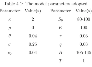
Table 4.1: The model parameters adopted Parameter Value(s) Parameter Value(s)

2 S0 80-100 0 K 100 0.04 r 0.03 0.25 q 0.03 v0 0.04 B 105-145 T 1

For tested parameters (u) near 800 is almost zero (see Figure 4.1), so the choice a = 800 is adequate. For x 2 [ b; b], we have to look at f(x): It is also a well behaved fast converging function. We do not need the negative x values for the calculation of V0, but it is easier to work with them in the

FFT algorithm. From the analysis above we can observe that it would be bene…cial to discreticise the functions unevenly. Unfortunately, this is not compatible with the FFT algorithm. The d1 integral in a discrete form is

d1(x) = 1 2 Z R e ixu ₁(u)du 1 2 a Z a e ixu ₁(u)du 1 2 N 1 X n=0 e ixun 1(u) u; (4.2)

where u is a u step, i.e. un = (n N₂) u for n = 0; ::; N with N intervals

for [ a; a]. The sum (4.2) is almost the same as equation (4.1). All we need to do is to choose wisely the x points:

xp = (p

N

2) x and x u = 2

(67)

for p = 0; ::; N 1. With these choices, X[p] = 1 2 N_X1 n=0 e i(n N2) u(p N 2) 2 N u 1(u) u = 1 2 N_X1 n=0 e 2 iN (np+ N 2 4 N p 2 N n 2 ) 1(u) u: (4.4)

Note that the exponential parcels are:

1. e 2 iN np ! ready for the FFT 2. e 2 iN4 = 1 ! if we choose N = 22k 3. e+ ip = ( 1)p _{! independent of n} 4. e+ in_{= ( 1)}n

Combining all the terms, equation (4.4) becomes X[p] = 1 2 ( 1) p N_X1 n=0 e 2 iN np[( 1)n 1(un)]:

Hence, the application of the FFT to

U [n] = ( 1)n ₁(un)

will give us the sum (integral estimation) at point xp. Note that the second

condition from (4.3) is the trade-o¤ between the number of points N (speed) and the values of x and u (accuracy). These choices have to be well

made and veri…ed or we will get some “impressive” results. For our tested parameters, we choose N = 28 _and

(68)

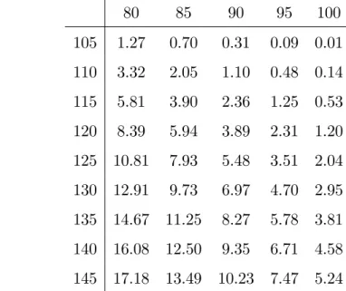
The double barrier option price in this case can be computed by the Liptons eigenfunction expansion method from [Lipton, A. (2001)] presented in Appendix 5.4, with the lower barrier close to zero (L = 0:001) and the upper barrier U = B. The error level was established at 10 13_{. The results}

are presented in the Table 4.2.

Table 4.2: The barrier option price via Liptons eigenfunction expansion, (Spot 80-100, Barrier 105-145) 80 85 90 95 100 105 1.27 0.70 0.31 0.09 0.01 110 3.32 2.05 1.10 0.48 0.14 115 5.81 3.90 2.36 1.25 0.53 120 8.39 5.94 3.89 2.31 1.20 125 10.81 7.93 5.48 3.51 2.04 130 12.91 9.73 6.97 4.70 2.95 135 14.67 11.25 8.27 5.78 3.81 140 16.08 12.50 9.35 6.71 4.58 145 17.18 13.49 10.23 7.47 5.24

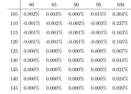
The di¤erences between equation (3.53) and our algorithm in Appendix 5.5 are presented in table 4.3.

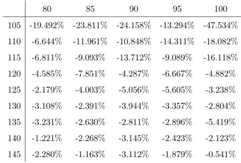
In comparison, the Monte-Carlo simulation from Appendix 5.5 with N = 105 _{and the jump interval} _{t = 1=300} _{is presented in Table 4.4.}

As expected, due to the full truncation algorithm, the Monte-Carlo sim-ulation is less accurate.

(69)

Table 4.3: The di¤erence between case 1 formula and Liptons eigenfunction expansion, (Spot 80-100, Barrier 105-145)

80 85 90 95 100 105 0.002% 0.003% 0.006% 0.015% 0.304% 110 -0.001% -0.002% -0.002% -0.003% 0.237% 115 -0.001% -0.001% -0.001% -0.001% 0.163% 120 -0.001% -0.001% -0.001% -0.001% 0.105% 125 0.000% 0.000% 0.000% 0.000% 0.067% 130 0.000% 0.000% 0.000% 0.000% 0.044% 135 0.000% 0.000% 0.000% 0.000% 0.031% 140 0.000% 0.000% 0.000% 0.000% 0.024% 145 0.000% 0.000% 0.000% 0.000% 0.020%

4.3 Case 3

For the general case, we will be dealing with equations (3.63) and (3.62). In more comfortable notation

V0 e rT ZZ R2 + f3(x; y) d3(x; y)dxdy; (4.5) with f3(x; y) = S0I1;1(x; y) KI1;0(x; y) S0I2;1(x; y) + KI2;0(x; y) d3 = dv2_;v T(x; y) = g(y) Z R

(70)

Table 4.4: The di¤erence between the Monte-Carlo simulation and Liptons eigenfunction expansion, (Spot 80-100, Barrier 105-145)

80 85 90 95 100 105 -19.492% -23.811% -24.158% -13.294% -47.534% 110 -6.644% -11.961% -10.848% -14.311% -18.082% 115 -6.811% -9.093% -13.712% -9.089% -16.118% 120 -4.585% -7.851% -4.287% -6.667% -4.882% 125 -2.179% -4.003% -5.056% -5.605% -3.238% 130 -3.108% -2.391% -3.944% -3.357% -2.804% 135 -3.231% -2.630% -2.811% -2.896% -5.419% 140 -1.221% -2.268% -3.145% -2.423% -2.123% 145 -2.280% -1.163% -3.112% -1.879% -0.541%

where Ij;k is given for case 3, in Appendix 5.1, and

g(y) = 1

2 e

L +(v0 y) 2_;

h(y; u) = e Ld (v0+y)de+_2e ₍ye

d v0 )L 12I 2L 1( 4d 2_e p yv0e d ):

From equation (4.6) for the …xed y we have the same problem as in case 1 for the function d1(x). Hence, we will apply the FFT for each y and create

a (x; y) grid for the integral in (4.5). We can summarize our algorithm as:

1. Fix yp

2. Calculate d3(xi; yp)through the FFT

(71)

4. Combine all the d3(xi; yp) values with f3(xi; yp)and use the 2D

trape-zoidal rule

5. Hope that everything goes well, as planned

Unfortunately the …nal step was very hard to accomplish. The algorithm is hard to calibrate.

(72)

5 Appendix

Theorem 1 Ito’s Lemma or Ito’s Formula. Let dX(t) = dt + dB(t) be an n-dimensional Itô process. Let g : [0; 1[ Rn

! Rp _{be a C}2 _{map. Then}

the process

Y (t; w) = g(t; X(t))

is again the Itô process whose component Yk, is given by

dYk = @gk @t (t; X)dt + X i @gk @Xi (t; X)dXi+ 1 2 X ij @gk @Xi@Xj ; where dBidBj = ijdt and dBidt = dtdBi = 0.

For reference see [Øksendal, B. (2002)].

5.1 The inner expectation formulas

Case 1: r = q and = 0 I1;1 = N log(S0 K) + 1 2 2_{(T )} (T ) ! N log( S0 B) + 1 2 2_{(T )} (T ) ! I1;0 = N log(S0 K) + 1 2 2_{(T )} (T ) ! N log( S0 B) + 1 2 2_{(T )} (T ) ! I2;1 = B S0 " N log( B2 S0K) + 1 2 2_{(T )} (T ) ! N log( B S0) + 1 2 2_{(T )} (T ) !# I2;0 = S0 B " N log( B2 S0K) + 1 2 2_{(T )} (T ) ! N log( B S0) + 1 2 2_{(T )} (T ) !# :

(73)

Case 2: r 6= q and = 0 I1;1 = exp((r q)T ) " N log( S0 K) + (r q)T + 1 2 2_{(T )} (T ) ! N log( S0 B) + (r q)T + 1 2 2_{(T )} (T ) !# I1;0 = " N log( S0 K) + (r q)T 1 2 2_{(T )} (T ) ! N log( S0 B) + (r q)T 1 2 2_{(T )} (T ) !# I2;1 = exp((r q)T ( 2 2_{(T )}log( B S0 ) + 1)) B S0 " N log( B2 S0K) + (r q)T + 1 2 2_{(T )} (T ) ! N log( B S0) + (r q)T + 1 2 2_{(T )} (T ) !# I2;0 = exp((r q)T ( 2 2_{(T )}log( B S0 ) + 1)) S0 B " N log( B2 S0K) + (r q)T 1 2 2_{(T )} (T ) ! N log( B S0) + (r q)T 1 2 2_{(T )} (T ) !# :

Case 3: r 6= q and arbitrary

I1;1 = exp( 1 2 2 2 2_{(T ) + q)} " N log( S0 K) + q + 2 2 2(T ) 2 (T ) ! N log( S0 B) + q + 2 2 2(T )) 2 (T ) !# I1;0 = " N log( S0 K) + q 2 (T ) ! N log( S0 B) + q 2 (T ) !# I2;1 = exp( 1 2 2 2 2_{(T ) + q)(}B S0 ) 2q 2 2 2(T ) +2 " N log( B2 S0K) + q + 2 2 2(T ) 2 (T ) ! N log( B S0) + q + 2 2 2(T ) 2 (T ) !# I2;0 = ( B S0 ) 2q 2 2 2(T ) " N log( B2 S0K) + q 2 (T ) ! N log( B S0) + q 2 (T ) !# ;

(74)

where

q = c1T + c2 2(T ) + c3(vT + v0):

Proposition 2 (Novikov’s Condition) For Xt adapted process, on the

probability space ( ; Ft; P) and BM Wt, if

E eR T0 jXtj2dt <1 then Zt= e t R 0 XsdWs 1₂ t R 0 X2 sds

is a Martingale. See e.g. [Øksendal, B. (2002)], and the reference therein.

5.2 Feynman-Kac Theorem

Theorem 3 (Feyman-Kac) Consider the stochastic di¤erential equation dX(t) = (t; X(t))dt + (t; X(t))dW (t)

Let h(y) be a Borel-measurable function. Fix T > 0, and let t 2 [0; T ] be given. De…ne the function

g(t; x) = Et;x[h(X(T )] = [E[h(X(T )jF(t)];

(We assume that Et;x[h(X(T )] < _{1 for all t and x). Then g(t; x) satis…es} the PDE gt(t; x) + (t; x)gx(t; x) + 1 2 2_{(t; x)g} xx(t; x) = 0

and the terminal condition

g(T; x) = h(x) _8x

Barrier option pricing via heston model