NUMERICAL METHOD TO PREDICT VOID FORMATION DURING THE LIQUID COMPOSITE MOLDING PROCESS

NUMERICAL METHOD TO PREDICT

VOID FORMATION DURING THE LIQUID

COMPOSITE MOLDING PROCESS

Zuzana Dimitrovová1 and Suresh G. Advani2

1

Researcher of IDMEC / IST and Invited Auxiliary Professor of DEM / ISEL Av. Rovisco Pais, 1, 1049-001 Lisbon, Portugal: [email protected]

2

Professor, Department of Mechanical Engineering and Center for Composite Materials University of Delaware, Newark, DE 19716: [email protected]

Corresponding author’s email: [email protected]

SUMMARY: Void formation during the injection phase of the liquid composite molding process can be explained as a consequence of the non-uniformity of the flow front progression. This is due to the dual porosity within the fiber perform (spacing between the fiber tows is much larger than between the fibers within in a tow) and therefore the best explanation can be provided by a mesolevel analysis, where the characteristic dimension is given by the fiber tow diameter of the order of millimeters. In mesolevel analysis, liquid impregnation along two different scales; inside fiber tows and within the open spaces between the fiber tows must be considered and the coupling between the flow regimes must be addressed. In such cases, it is extremely important to account correctly for the surface tension effects, which can be modeled as capillary pressure applied at the flow front. Numerical implementation of such boundary conditions leads to ill-posing of the problem, in terms of the weak classical as well as stabilized formulation. As a consequence, there is an error in mass conservation accumulated especially along the free flow front. A numerical procedure was formulated and is implemented in an existing Free Boundary Program to reduce this error significantly.

KEYWORDS: void formation, surface tension, capillary pressure, mass conservation, free boundary flow, mesolevel analysis, dual porosity.

INTRODUCTION

Liquid Composite Molding is a composite manufacturing process in which fiber preforms consisting of stitched or woven bundles of fibers, known as fiber tows, are stacked in a closed mold and a polymeric resin is injected to impregnate all the empty spaces between the fibers. Fiber tows are usually millimeters in diameter and consist of bundles of 2000 to 5000 fibers [1]. An important step is to ensure saturation of all the fiber tows and regions in between them in order to avoid voids formation. Due to the dual porosity in woven fiber preforms, resin progression is not uniform, and a transition region where the flow has not yet stabilized and saturated, is formed along the macroscopic flow front. This region is very sensitive to voids formation. The best way to analyze this flow is at the mesolevel, i.e at the scale of fiber tows. FPCM-7 (2004)

The 7th International Conference on Flow Processes in Composite Materials

MESOLEVEL ANALYSIS

Fig.1 Flow domain, regions and boundaries designation

In mesolevel analysis, liquid flowing along two different scales must be considered. Single scale porous media (fiber tows represented in Fig. 1 by grey half-circles) and open spaces (white spaces) are presented in the same unit cell which will allow one to couple the flow in these two different regimes. Fiber tows have uniformly distributed pores, therefore sharp flow front can be assumed as the resin impregnates. Moreover quasi steady state assumption can be exploited. As the flow is slow, inertia terms can be neglected, implying that one can assume Stokes flow in the inter-tow spaces S_t

k

Ω (white space between Γin and _tS

k

Γ ) and Darcy’s flow in saturated intra-tow region B_t

k

Ω which need to be solved at each discretized time tk. In fact, Darcy’s law must be

modified to Brinkman’s equations, in order to account for viscous stress at the interface between these two regions ( S B

tk

−

Γ ), which rapidly decreases with the distance from S B tk

−

Γ . In summary, the following equations must be satisfied at each time step, tk:

in inter-tow spaces: ∇⋅v=0 and ∇p=μΔv in S_t

k

Ω

(Stokes equations), (1) in intra-tow spaces: ∇⋅vD =0 and ∇pf =μΔvD−μK−1⋅vD in B_t

k

Ω

(Brinkman’s equations), (2) where v is local velocity vector, p is local pressure, μ is resin viscosity and ∇ stands for spatial gradient, Δ=∇⋅∇. vD is Darcy’s velocity vector, i.e. the phase averaged velocity related to the intrinsic phase average vf by vD=φtvf, where φt is intra-tow porosity. pf stands for intrinsic phase

average of the local pressure and K is absolute permeability tensor.

If fibers inside the tows are rigid, impermeable and stationary, the following boundary conditions, under usual omission of the air pressure, must be fulfilled at the free front:

0

σv =

t and

(

)

n

v_{⋅ ⋅ − =σ − ≈− =− =− γ} n

n

σ at S

tk

Γ , (3)

pf=Pc at ΓtBk. (4)

Here σv is local viscous stress, v t

σ tangential vector of the viscous stress vector, v n

σ normal component of the viscous stress and n the outer unit normal vector to the free front in Stokes region _tS

k

Γ . pc and Pc stand for local and global (homogenized) capillary pressure, γ is resin

fiber tow

symmetry

flow direction

fiber tow in

Γ

S tk

Ω

B tk

Ω

B S tk

−

Γ

B tk

Γ

S tk

Γ

symmetry

B tk

Ω

surface tension and H is mean curvature. Progression of the free boundary can be determined according to:

0 f t

f Dt Df

= ∇ ⋅ + ∂ ∂

= v at _tS

k

Γ , (5)

0 f t

f Dt Df

t D

= ∇ ⋅ φ + ∂ ∂

= v at _tB

k

Γ , (6)

where f(x(t),t)=0 is implicit function describing the moving sharp flow front (dark line in Fig. 1), x is spatial variable and t is time. Other boundary conditions such as symmetry, periodicity and inlet conditions at Γin are related to the particular problem under consideration.

We have formulated the governing equations for free boundary flows in intra- as well as inter-tow spaces and developed numerical techniques to address the movement of the flow at the mesolevel scale which we call the Free Boundary Program (FBP). Numerical simulations can track the advancement of the resin front promoted by both hydrodynamic pressure gradient and capillary action [2-5]. In such simulations it is extremely important to account correctly for the surface tension effects, which can be modeled as capillary pressure applied at the flow front. Unfortunately essential boundary conditions of this kind make the problem ill-posed, in terms of the weak classical as well as stabilized formulation. As a consequence there is an error in mass conservation accumulated especially along the free front. This can affect significantly normal velocities at the free front and distort the next front shape. Due to the explicit integration along the time scale, such errors are irreversible. Several stabilization techniques were implemented in FBP to eliminate this effect [3-5]. In this article we will present more appropriate techniques for stabilization, based on weak formulation of the problem. The methodology implemented in Darcy’s region is well-known, although rarely used in real simulations. It is presented e.g. in [6]. The recalculated outlet velocities have superior convergence properties [7]. In Stokes region the correction of the outlet velocities we are presenting have not yet been published to our knowledge. Both methodologies are implemented in FBP.

FLOW FRONT RECALCULATION AND CORRECTION

Following [6], outlet normal velocities can be recalculated in Darcy’s region according to:

(

)

(

) ( )

n h

Pˆ q q

L p , q B v

~ ,

q B

k

t = − ∀ ∈

Γ . (7)

B and L represent bi-linear and linear form of the weak formulation, new outlet velocities with superior convergence properties are v~_nD,h, qh is trial pressure and pf,h is the solution already

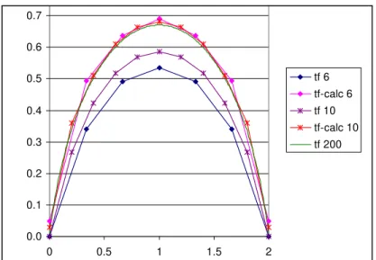
obtained in a standard way. Trial pressures space, Pˆ , consists now solely from functions h originally omitted because of the pressure essential boundary condition. Efficiency of this technique can be shown on a simple example:

[ ] [ ]

1

u= − × −

Δ ,

[ ] [ ]

(

)

boundary the

at 0

u= ∂ − × − . (8)

0.0 0.1 0.2 0.3 0.4 0.5 0.6 0.7

0 0.5 1 1.5 2

tf 6 tf-calc 6 tf 10 tf-calc 10 tf 200

Fig. 2 Normal thermal fluxes of the problem specified in (8). Notice that recalculated fluxes on 6x6 and 10x10 meshes (tf-calc 6 and tf-calc 10) do as good a job as a mesh of 200x200 (tf 200)

In the Stokes region the following scheme is used:

(

) (

)

n h

Pˆ q ,

q w

, q S

k

t = ∇⋅ ∀ ∈

Γ v ,

h n h n h

n v w v

~ _{= − ,} (9)

where w is an auxiliary value of the normal velocity, used to correct the originally obtained h_n

normal velocities, v . In this case incompressibility condition is completely separated from the h_n weak formulation. Efficiency was verified directly on ANSYS fluid element FLUID 141, where pressure and velocities are nodal variables. Test problem for unit viscosity and mass free fluid is specified in Fig. 3a) and results are shown in Fig. 3b).

Fig. 3 (a) Fluid problem definition, (b) original values vy 5, vy 10 and vy 50 on 5x5, 10x10 and 50x50 quad meshes and recalculated vy-calc 5 and vy-calc 10 outlet normal velocities

-1500 -1000 -500 0 500 1000

0 0.5 1 1.5 2 vy 5

vy-calc 5 vy 10 vy-calc 10 vy 50 p=0

inlet v=10 2nd order polinom

vn=0

no-slip v=0

p=10000

a)

Also here the recalculated outlet normal velocities fit the solution well for the very fine mesh. In this test problem pressure does not correspond to the capillary pressure, because the aim was only to test the efficiency of such methodology.

CONCLUSION

Presented stabilization techniques are very efficient as shown in the simple test examples. They permit calculation of frontal normal velocities with sufficient precision even for coarse meshes. They are included in the post-processing part of FBP. Their implementation ensures better mass conservation at the global as well as the local level. It makes it possible to obtain a front shape that is not only more exact but also smoother. The computational time is reduced as coarser meshes can be used to obtain stable and accurate answers and it also allows one to step through larger time steps during the impregnation process.

ACKWNOLEDGMENTS

Firstly named author would like to thank to the Portuguese institution for founding research Fundação para a Ciência e a Tecnologia for the scholarship allowing developing this work.

REFERENCES

1. S. G. Advani, M. V. Bruschke and R. S. Parnas, “Resin transfer molding”, In: Advani SG, editor. Flow and rheology in polymeric composites manufacturing. Amsterdam, Elsevier Publishers, 1994, pp. 465-516.

2. Z. Dimitrovová and S. G. Advani, “Analysis and characterization of relative permeability and capillary pressure for free surface flow of a viscous fluid across an array of aligned cylindrical fibers”, Journal of Colloid and Interface Science, Vol. 245, 2002, pp. 325-337.

3. Z. Dimitrovová and S. G. Advani, “Free boundary viscous flows at micro and mesolevel during liquid composites molding process”, CD of communications of 14th International Conference on Composites Materials, San Diego, California, EUA, 2003.

4. Z. Dimitrovová and S. G. Advani, “Numerical simulation of free boundary viscous flows at all length scales of LCM process”, CD de comunicações do 3th International Conference on Computational & Experimental Engineering and Sciences, Corfu, Grécia, 2003.

5. Z. Dimitrovová and S. G. Advani, “Mesolevel analysis of the transition region formation and evolution during the liquid composite molding process”, Computers & Structures, accepted, 2004.