Lisbon, Portugal, 5–8 June 2006
POST-PROCESSING TECHNIQUES SUITABILITY FOR MESOLEVEL
FREE BOUNDARY FLOWS
Zuzana Dimitrovová1
1
UNIC, Department of Civil Engineering New University, Monte Caparica, Portugal
Keywords: Post-processing techniques, Darcy’s flow, Stoke’s flow, Free boundary flows, Mesolevel analysis, Capillary pressure, Liquid composite molding.
1 INTRODUCTION
Reliable flow simulation software is inevitable to determine an optimal injection strategy in Liquid Composite Molding processes. Void formation during the injection phase can be explained as a consequence of the non-uniformity of the flow front progression. Origin of this fact lies in the dual porosity of the fiber preform and therefore the best explanation can be provided by a mesolevel analysis. In the mesolevel analysis different flow regimes must be considered and linked together at each time step. In such simulation it is extremely important to account correctly for the surface tension effects, which can be modeled as capillary pres-sure applied at the free flow front, [1-2].
Numerical techniques to address the movement of the flow were already developed in the Free Boundary Program (FBP) [2-4]. Numerical simulations can track the advancement of the resin front promoted by both hydrodynamic pressure gradient and capillary action. Base analysis is solved in commercial code ANSYS. However, capillary action implementation brings numerical difficulties, when continuous Galerkin method is used. This can be over-come by post-processing the free-boundary normal velocities, resulting in superior conver-gence results. Post-processing a finite element solution is a well-known technique, which consists in a recalculation of the originally obtained quantities such that the rate of conver-gence increases without the need for expensive remeshing techniques [6-9]. Post-processing is especially effective in problems where better accuracy is required for derivatives of nodal variables in regions where Dirichlet essential boundary condition is imposed strongly [6]. Consequently, such an approach can be exceptionally good in modeling of resin infiltration under quasi steady-state assumption, because only free-front normal velocities are necessary to advance the resin front to the next position.
2 MESOLEVEL ANALYSIS
In the mesolevel analysis single scale porous media, fiber tows, (shown in Figure 1 by grey half-circles) and open spaces (white spaces) are presented together in the flow domain. Fiber tows have uniformly distributed pores, therefore sharp flow front can be assumed as the resin impregnates. As the flow is slow, inertia terms can be neglected, thus one can assume Stoke’s flow in the currently filled inter-tow spaces St
k
Ω (white space between Γin and tS
k
Γ ) and
Brinkman’s flow in the saturated intra-tow region; Bt
k
Ω . The interface between these two re-gions is designated as tS B
k −
Γ .
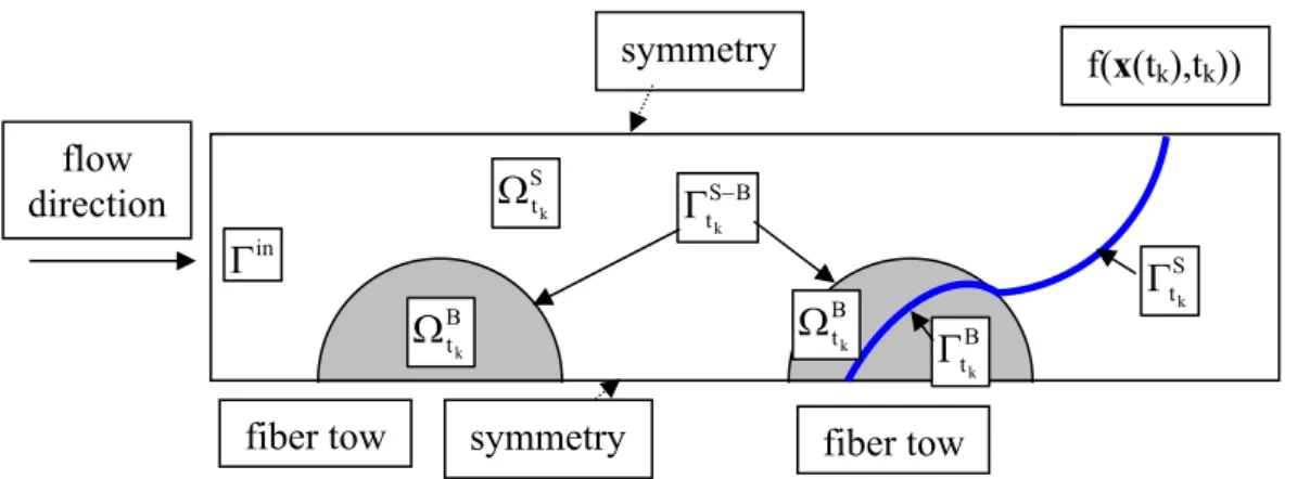
Figure 1: Flow domain, regions and boundaries designation.
fiber tow
symmetry
flow direction
fiber tow
in
Γ
S tk
Ω
B tk
Ω
B S tk −
Γ
B tk
Γ
S tk
Γ
symmetry
B tk
Ω
In summary, the following equations must be satisfied at each time step, tk:
in inter-tow spaces: ∇⋅v=0 and ∇p=μΔv in St
k
Ω , (1)
in intra-tow spaces: ∇⋅vD =0 and ∇pf =μΔvD−μK−1⋅vD in Bt
k
Ω , (2)
where v is local velocity vector, p is local pressure, μ is resin viscosity and ∇ stands for spa-tial gradient, Δ=∇⋅∇. vD is Darcy’s velocity vector, i.e. the phase averaged velocity related to the intrinsic phase average vf by vD=φtvf, where φt is the intra-tow porosity. pf stands for the
intrinsic phase average of the local pressure and K is the absolute permeability tensor.
If fibers inside the tows are rigid, impermeable and stationary, the following boundary conditions, under usual omission of the air pressure, must be fulfilled at the free front:
0
σv =
t and
(
)
p p p pc 2 Hv n
v⋅ ⋅ − =σ − ≈− =− =− γ
n n
σ at tS
k
Γ , (3)
pf=Pc at ΓtBk. (4)
Here σv is local viscous stress,σvt tangential vector component of the viscous stress vector,
v n
σ normal component of the viscous stress and n is the outer unit normal vector to the free front in Stokes region tS
k
Γ . pc and Pc stand for the local and global (homogenized) capillary
pressure, γ is the resin surface tension and H is the mean curvature. Progression of the free boundary can be determined according to:
0 f t
f Dt
Df + ⋅∇ =
∂ ∂
= v at tS
k
Γ , (5)
0 f t f Dt Df t D = ∇ ⋅ φ + ∂ ∂
= v at tB
k
Γ , (6)
where f(x(t),t)=0 is implicit function describing the moving sharp flow front (dark bold line in Figure 1), x is spatial variable and t is time. Other boundary conditions such as symmetry, pe-riodicity and inlet conditions at Γin are related to the particular problem under consideration.
3 NUMERICAL SIMULATION
The governing equations for free boundary flows in intra- as well as inter-tow spaces were formulated and numerical techniques to address the movement of the flow at the mesolevel scale were developed. The corresponding software is named as Free Boundary Program (FBP). Numerical simulations can track the advancement of the resin front promoted by both hydro-dynamic pressure gradient and capillary action [2-4].
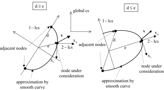
Figure 2: Two kinds of approximation of the flow front by a smooth curve. t g v x g v v n t t n ∂ ∂ = = ∂ ∂
− . (7)
In the explicit approach, the new nodal position is determined in the normal direction as:
(
)
kk 1
k n,t k 1 k n,t t
,
n x t t v
x + = + + − . (8)
The smooth curve approximation as described above is repeated, now for the new front, and the surface curvature is determined in order to calculate the capillary pressure, which is then applied according to (3) as piece-wise linear at each frontal element edge, or alternatively condition (4) is imposed directly. Finally, the other boundary conditions are applied and the base problem is solved for in the new domain.
Unfortunately, essential boundary conditions (3-4) cause numerical problems in the weak, classical as well as stabilized, formulation. As a consequence, there is an error in mass con-servation accumulated especially along the free front. This can affect significantly normal ve-locities at the free front and distort the next front shape. Due to the explicit integration along the time scale, such errors are irreversible. Several stabilization techniques were implemented in FBP to eliminate this effect [2, 4]. More appropriate techniques for stabilization, based on weak formulation of the problem, are offered by post-processing techniques. Their suitability was already examined in [10-12].
4 POST-PROCESSING TECHNIQUES
4.1 Darcy´s flow
In the region where Darcy’s flow is fully developed, normal component velocities on free boundary, where homogenized capillary pressure is imposed, can be recalculated from the following weak formulation [5-9]:
(
D,h)
(
h f,h) ( )
h h hn
h,~v Bq ,p Lq q Pˆ
q B
k
t = − ∀ ∈
Γ , (9)
adjacent nodes v cs global d e e
d≥ d≤e
where B and L stand for bi-linear and linear form of the weak formulation. Recalculated com-ponents v~nD,h have superior convergence properties, in terms specified in [5]. Space of trial functions Pˆ includes now only the ones, which where omitted from the previous formulation h due to the essential boundary condition imposed on tB
k
Γ . Right hand side of Equation (9) can be calculated directly from the original solution pf,h; left hand side of the same equation re-quire only integration along the free boundary, thus the new values can be obtained as a part of post-processing.
For Darcy’s flow analogy with thermal analysis can be exploited, thus pressure can be sub-stituted by the temperature, θ, and Darcy’s velocity by the heat flux. In the literature, effi-ciency of technique (9) is usually shown on simple problems, which have analytical solution, like for instance:
(
1 x) (
21 y)
in[ ] [ ]
1,1 1,12 − 2 + − 2 − × −
= θ
Δ , (10)
[ ] [ ]
(
1,1 1,1)
on
0 ∂ − × −
=
θ , (11)
with the analytical solution as:
(
2)(
2)
y 1 x
1− −
− =
θ . (12)
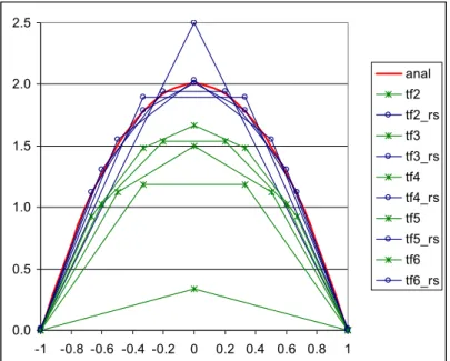
When uniform mesh of square elements is used on the square domain of this problem, symmetry can be exploited and therefore equations related only to one side of the domain can be solved. Recalculated flux has very good convergence properties, although the external normal is not defined in the corners. Results are shown in Figure 3.
0.0 0.5 1.0 1.5 2.0 2.5
-1 -0.8 -0.6 -0.4 -0.2 0 0.2 0.4 0.6 0.8 1
anal tf2 tf2_rs tf3 tf3_rs tf4 tf4_rs tf5 tf5_rs tf6 tf6_rs
Figure 3: Original and recalculated heat flux on one side of the square domain of problem (10-11).
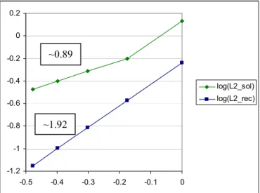
relative error is only 1.37%, except for the corners. Improved convergence in “log-log” plot is shown in Figure 4.
-1.2 -1 -0.8 -0.6 -0.4 -0.2 0 0.2
-0.5 -0.4 -0.3 -0.2 -0.1 0
log(L2_sol) log(L2_rec)
Figure 4: Log-log plot of L2-norm against element size for original (“sol”) and recalculated (“rec”) solution.
Efficiency in this case is impressive, however, it should be remarked, that in this problem, (i) boundary is straight, except for the corners; (ii) Dirichlet boundary condition is homogene-ous and (iii) there is a source term. The biggest distortion from the analytical solution in this example is located in the corners, where even the original solution meets the analytical zero value better than the recalculated one. These differences look insignificant in Figure 3, due to the scale. In this particular case, however, implementing the technique suggested in [8] can solve the corner problem.
In practical problems related to the flow simulation there is no source term, Dirichlet con-dition is non-homogeneous as it represents the applied capillary pressure and the free bound-ary is not straight. It can be somewhat non-smooth, also due to the discretization. Implementing the technique from [8] is difficult and not worthwhile. Recalculated results can be even worse, as was tested on some simple problems.
Effect of the smoothness of the Dirichlet condition was studied in [12]. Functions out of C1 cause analytical singularity, consequently post-processing cannot give reasonable results and the new values oscillate along the “exact” solution, as can be demonstrated in the following problem:
[ ] [ ]
1,1 1,1 in0 − × −
= θ
Δ , 0 onx 1andy
[ ]
1,1n = =± ∈ −
∂ θ ∂
, (13)
[ ]
1,1 xand 1 y for 10
n =− =− ∈ −
∂ θ ∂
, θ
( )
x =100(
1− x)
for y=1andx∈ −1,1 . (14)Here the imposed function is piece-wise linear and causes singularity in the middle and at the corners of the corresponding boundary. Analytical solution was approximated by numerical results from 200х200 mesh. Results are separated to even and odd divisions of the square do-main and are summarized in Figures 5-6. Legends obey the same rules as in Figures 3-4. It is seen that neither the recalculated values, nor the convergence exhibit the expected properties.
~0.89
-300 -200 -100 0 100 200 300
0.0 0.5 1.0 1.5 2.0
anal
tf5
tf5_r
tf7
tf7_r
tf9
tf9_r
-300 -200 -100 0 100 200 300
0.0 0.5 1.0 1.5 2.0
anal tf4
tf4_r
tf6
tf6_r
tf8
tf8_r
tf10
tf10_r
Figure 5: Original and recalculated flux of problem (13-14).
1.4 1.6 1.8 2.0 2.2 2.4
-0.7 -0.6 -0.5 -0.4 -0.3
log(L2_sol) log(L2_rec)
Figure 6: Log-log plot of L2-norm against element size for original (“sol”) and recalculated (“rec”) solution of problem (13-14).
As infiltration problem has a physical base, one is allowed to assume, that capillary pres-sure can be estimated by sufficiently smooth function, namely by function from C1. If more-over extension of the problem should be possible by symmetry or periodicity, side derivatives must be zero. Consequently there will be no corner problem and no singularities. As a conclu-sion, additional smoothing have to be added to the estimated capillary pressure, before its numerical application.
Another complication in post-processing techniques lies in permeability discontinuity. This was also examined in [12] and suggestions how to overcome arising problems were presented.
Even more perturbation can be caused by non-smooth front. Several cases were studied numerically. As remarked in [8], the corners, where the outer normal is not well-defined must be treated separately. The methodology suggested there is not very convenient to implement and it does not yield satisfactory results. In fact in FE approach, after discretization there is rarely possible to define uniquely the outer normal. It could be estimated as in FBP, as ex-plained in Section 3, but this would not help to improve the post-proceeded results. Therefore another technique is suggested in this paper. Its efficiency is demonstrated on the following test case.
Next figure shows some randomly created free boundary front in Darcy’s region. Simple
~0.74-76
case is tested with constant pressure at the inlet and constant pressure at the outlet boundary. Results are obtained by analogous thermal analysis. In this case all characteristics appear only as parameters, therefore dimensionless 10 is applied at the inlet, 0 at the outlet and permeabil-ity is characterized by unit. Case is tested on rough triangular mesh (Figure 7). In order to evaluate the solution correctness on this rough mesh, absolute error in flux is shown in Figure 8. It is seen that this error is quite high, it is concentrated around the free boundary, especially in sharp corners.
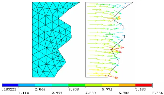
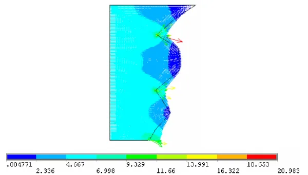
Figure 7: FE mesh and flux arrows of the test case original solution.
Figure 8: Absolute flux error of the test case original solution.
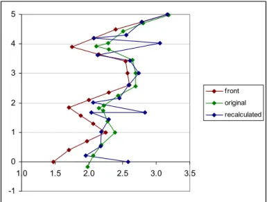
-1 0 1 2 3 4 5
1.0 1.5 2.0 2.5 3.0 3.5
front
original
recalculated
Figure 9: New front from original and recalculated in standard way outlet flux of the test case solution.
Improved methodology is therefore suggested, accounting for the actual angle forming the filled region around each frontal node. This technique has not been published yet. Rigorous proof is still in preliminary stage. However, it can be seen that with this improvement imple-mented, the recalculated front practically fits the “exact” solution, which was obtained on very fine mesh, in fact, element size was 10 times lower. In addition, improved recalculated solution removes the local disturbance of the “exact” solution at the sharp corners, which can be clearly observed in Figure 10.
-1 0 1 2 3 4 5
1.0 1.5 2.0 2.5 3.0 3.5
front
original
recalculated
"exact"
Figure 11: Flux arrows of the test case solution on fine mesh, designated as “exact” solution.
4.2 Stoke´s flow
The methodology implemented in Stoke’s region uses the following scheme, [10-12]:
(
h) (
h h)
h hn h
Pˆ q ,
q w
,
q S
k
t = ∇⋅ ∀ ∈
Γ v , hn
h n h
n v w
v
~ = − , (15)
where w is an auxiliary value, which is used for the correction of the originally calculated hn velocities, v . Equation (15) is similar to Equation (9), but in this case incompressible condi-hn tion is completely separated from the weak formulation of Stoke’s problem. It is proven in [10] that in one-dimensional case such recalculation leads an analytical value. Efficiency of the technique on smooth front with C1 Dirichlet boundary condition was shown in [12]. Improved methodology on non-smooth front presented in the previous section is also applicable here. The rigorous proof is still under examination.
5 CONCLUSION
REFERENCES
[1] S.G. Advani, Z. Dimitrovová, Role of Capillary Driven Flow in Composite Manufactur-ing, in Surface and Interfacial Tension: Measurement, Theory and Applications, ed. S. Hartland, Surfactant Science Series, 119, 263-312, 2004, Marcel Dekker, Inc., NY.
[2] Z. Dimitrovová, S.G. Advani, Mesolevel analysis of the transition region formation and evolution during the liquid composite molding process, Computers & Structures, 82, 1333-1347, 2004.
[3] Z. Dimitrovová, S.G. Advani, Analysis and characterization of relative permeability and capillary pressure for free surface flow of a viscous fluid across an array of aligned cy-lindrical fibers, Journal of Colloid and Interface Science, 245, 325-337, 2002.
[4] Z. Dimitrovová, S.G. Advani, Free boundary viscous flows at micro and mesolevel dur-ing liquid composites molddur-ing process, International Journal for Numerical Methods in Fluids, 46, 435-455, 2004.
[5] I. Babuška, A. Miller, The post-processing approach in the finite element method - Part 1: Calculation of displacements, stresses and other higher derivatives of the displace-ments, International Journal for numerical methods in Engineering, 20, 1085-1109, 1984.
[6] T.J.R. Hughes, G. Engel, L. Mazzei, M.G. Larson, The continuous Galerkin method is
locally conservative, Journal of Computational Physics, 163, 467-488, 2000.
[7] G.F. Carey, Derivative calculation from finite element solution, Computer Methods in Applied Mechanics and Engineering, 35, 1-14, 1982.
[8] G.F. Carey, S.S. Chow, M.K. Seager, Approximate boundary-flux calculations,
Com-puter Methods in Applied Mechanics and Engineering, 50, 107-120, 1985.
[9] A. Mizukami, A mixed finite element method for boundary flux calculations, Computer
Methods in Applied Mechanics and Engineering, 57, 239-243, 1986.
[10] Z. Dimitrovová, S.G. Advani, Numerical Method to Predict Void Formation during The
Liquid Composite Molding Process, 7th International Conference on Flow Processes in
Composite Materials, Newark, Delaware, EUA, 269-274, 2004.
[11] Z. Dimitrovová, S.G. Advani, Mass Conservation Enhancement of Free Boundary
Mesolevel Flows during LCM Processes of Composites Manufacturing, 7th
Interna-tional Conference on ComputaInterna-tional Structures Technology, Lisbon, Portugal, 49-50,
2004.
[12] Z. Dimitrovová, Post-processing Techniques in Free Boundary Flows during Liquid
Composite Moulding Processes, 10th International Conference on Civil, Structural and