Abstract
Undesirable void formation during the injection phase of the liquid composite moulding process can be understood as a consequence of the non-uniformity of the flow front progression, caused by the dual porosity of the fibre perform. Therefore the best examination of the void formation physics can be provided by a mesolevel analysis, where the characteristic dimension is given by the fibre tow diameter. In mesolevel analysis, liquid impregnation along two different scales; inside fibre tows and within the open spaces between them; must be considered and the coupling between these flow regimes must be addressed. In such case, it is extremely important to account correctly for the surface tension effects, which can be modelled as capillary pressure applied at the flow front. Numerical implementation of such boundary conditions leads to ill-posing of the problem, in terms of the weak classical as well as stabilized formulation. As a consequence, there is an error in mass conservation accumulated especially along the free flow front. This contribution presents a numerical procedure, which was formulated and implemented in the existing Free Boundary Program in order to significantly reduce this error.
Keywords: void formation, surface tension, capillary pressure, mass conservation, free boundary flow, mesolevel analysis, dual porosity
1 Introduction
Liquid Composite Moulding is a composite manufacturing process in which fibre preforms consisting of stitched, woven or braided bundles of fibres, known as fibre tows, are stacked in a closed mould and a polymeric resin is injected to impregnate all the empty spaces between the fibres. Fibre tows are usually millimetres in diameter and consist of bundles of 2000 to 5000 fibres of few micrometers in
Mass Conservation Enhancement of
Free Boundary Mesolevel Flows during
LCM Processes of Composites Manufacturing
Z. Dimitrovovᆠand S.G. Advani‡ † IDMEC/IST and DEM/ISEL
Instituto Superior Técnico, Lisbon, Portugal ‡ Department of Mechanical Engineering
University of Delaware, Newark DE, United States of America
diameter [1]. An important step is to ensure saturation of all the fibre tows and regions in between them in order to avoid voids formation, which can drastically reduce the mechanical properties of the manufactured part. Due to the dual porosity of the fibre preform, resin progression is not uniform, and a transition region where the flow is not yet stabilized and saturated, is formed along the macroscopic flow front. This region is very sensitive to voids formation. The best way to analyze this flow is at the mesolevel, i.e. at the scale of the fibre tows [2].
The understanding can be separated into two basic flow directions: flow across and along fibre tows. In the case of flow across the fibre tows, experimental evidence shown in [3-5] and numerical results presented in [6-7] clearly demonstrate that filling of the fibre tows is delayed. Resin advance, although helped by strong intra-tow capillary pressure, must overcome a fibre arrangement with much lower intra-tow permeability; thus there could hardly exist some scenario, which would move the front more or less uniformly. It is also known [8] that very high surrounding pressure acting on the tows can significantly change the single fibres positions and actually close some spaces between them. Usually only a thin strip along the fibre tow circumference is filled when the primary resin front envelopes it, then the air is compressed inside the tow until it is balanced with the surrounding resin pressure. Hence the capillary action becomes the only factor that can drive the resin inside the tow. When the air pressure becomes higher than the surrounding pressure, the air can escape from the tow in the form of microvoids.
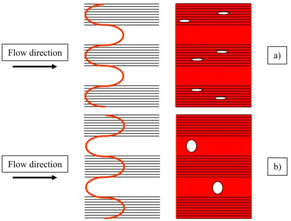
Figure 1: Inter-tow (a) and intra-tow (b) void formation Flow direction
Flow direction
a)
Nevertheless this is just an academic case. If the resin is not forced to flow only across the fibre tows, it will naturally choose the easier (higher permeability) direction, i.e. along the fibre tows in this case. In flow along fibre tows, permeability is much higher (four to ninety times) and capillary action is generally twice as strong as in flow across the tows. Therefore two situations can be found in flow along fibre tows [9-11]. Wicking flow front inside the fibre tow can be either advanced or delayed with respect to the primary front in the inter-tow spaces, which also pre-determinates the location and shape of emerging voids (Figure 1).
Because capillary action does not depend on the externally applied inlet conditions, but it is purely a function of the resin surface tension, contact angle and geometry, these two scenarios can be explained as follows. When the externally applied pressure or flow rate is relatively high, viscous action is dominant, wicking gradient is not so strong when compared to the hydrodynamic pressure gradient and therefore inter-tow spaces (the higher permeability regions) are filled first. On the other hand, under lower externally applied action, wicking flow can become dominant and resin advances more rapidly inside the tows. There must naturally exist a situation, when these actions are “equilibrated” and resin progresses more or less uniformly. It should be remarked in this context, that higher external conditions are used with the objective to reduce the filling time, as a main cost factor. On the other hand it is well known that lower external conditions are favourable for better accomplishment of the infiltration phase and quality of the part, because sufficient time must be given to the resin-fibre interaction to form an interface increasing the adhesion between the two phases. However, in very slow filling it is conceivable that the resin will cure and solidify before all the empty pores are filled. More about role of capillary driven flow in composites manufacturing can be found in [12].
In summary, it is obvious that in modelling of physics of the voids formation it is extremely important to account correctly for the capillary pressure influence.
2 Mesolevel analysis
2.1 Governing equations and the flow domain
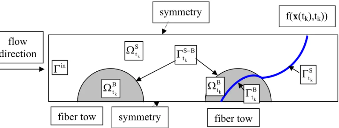
In mesolevel analysis, liquid flowing along two different scales must be considered. Single scale porous media (fibre tows represented in Figure 2 by grey half-circles) and open spaces (white spaces), corresponding to different flow regimes, are presented together in the flow domain. Therefore these two flow regimes have to be coupled in one analysis.
Fibre tows have uniformly distributed pores, therefore sharp flow front can be assumed as the resin impregnates. As the flow is slow, inertia terms can be neglected, implying that one can assume Stokes flow in the currently filled inter-tow spaces St
k
Ω (white space between Γin and tS
k
Γ ) and Darcy’s flow in the saturated intra-tow region; Bt
k
account for the viscous stress at the interface between these two regions ( tS B
k
−
Γ ). Viscous stress rapidly decreases with the distance from tS B
k
−
Γ . In summary, the following equations must be satisfied at each time step, tk:
Stokes equations in the inter-tow spaces: ∇⋅v=0 and ∇p=μΔv in St
k
Ω , (1) Brinkman’s equations in the intra-tow spaces: ∇⋅vD =0 and
D 1 D
f
p =μΔv −μK ⋅v
∇ −
in Bt
k
Ω , (2)
where v is the local velocity vector, p is the local pressure, μ is the resin viscosity and ∇ stands for the spatial gradient, Δ=∇⋅∇. vD is the Darcy’s velocity vector, i.e. the phase averaged velocity related to the intrinsic phase average vf by vD=φtvf,
where φt is the intra-tow porosity. pf stands for the intrinsic phase average of the
local pressure and K is the absolute permeability tensor.
Figure 2: Flow domain, regions and boundaries designation
If fibres inside the tows are rigid, impermeable and stationary, the following boundary conditions, under the usual omission of the air pressure, must be fulfilled at the free front:
0
σv =
t and
(
)
p p p pc 2 Hv n
v⋅ ⋅ − =σ − ≈− =− =− γ
n n
σ at tS
k
Γ , (3)
pf=Pc at ΓtBk. (4)
Here σv is the local viscous stress,σvt and σvn are the tangential vector and the normal component of the viscous stress vector at the free front, respectively, and n is the outer unit normal vector to the free front in Stokes region tS
k
Γ . pc and Pc stand for
the local and the global (homogenized) capillary pressure, γ is the resin surface tension and H is the mean curvature. Progression of the free boundary can be determined according to:
0 f t
f Dt
Df + ⋅∇ =
∂ ∂
= v at tS
k
Γ , (5)
0 f t f Dt Df t D = ∇ ⋅ φ + ∂ ∂
= v at tB
k
Γ , (6)
fiber tow symmetry flow direction fiber tow in Γ S tk Ω B tk Ω B S tk − Γ B tk Γ S tk Γ symmetry B tk Ω
where f(x(t),t)=0 is the implicit function describing the moving sharp flow front (bold blue line in Figure 2), x is the spatial variable and t is the time. Other boundary conditions such as symmetry, periodicity and inlet conditions at Γin are related to the particular problem under consideration.
2.2 The Free boundary program
We have formulated the governing equations for the free boundary flows in intra- as well as inter-tow spaces and developed numerical techniques to address the movement of the flow at the mesolevel scale, which we call the Free Boundary Program (FBP). Numerical simulations can track the advancement of the resin front promoted by both hydrodynamic pressure gradient and capillary action [2, 7, 12-14]. Quasi steady state assumption can be exploited in the full flow domain and explicit time integration is adopted along the time scale. FBP is thus concerned with the moving flow front, which requires results at time tk; approximation of the front at tk
locally by a smooth curve in order to determine outer normals for use in the kinematic free boundary condition (5-6); determination of the new resin front position at tk+1; approximation of this front locally in Stoke’s region again by a
smooth curve in order to determine its curvature; and application of the boundary conditions. Then the base analysis is solved by ANSYS FLOTRAN module and the process is repeated. FBP has to deal with the usual problems of moving mesh algorithms with re-meshing of the filled domain at each time step, like boundary identification, preventing of normal crossing, free boundary looping, etc.
ANSYS FLOTRAN can account for porous media influence by introduction of distributed resistance. Averaged values in Equations (2, 4, 6) are therefore important mainly from the theoretical viewpoint, while numerically either velocity or pressure maintain their meaning as nodal variables in both regions, preserving all necessary continuity requirements at tS B
k
−
Γ . In mesolevel simulations it is extremely important to account correctly for the surface tension effects, as pointed out in the Introduction.
correction of the outlet velocities we are presenting have not yet been published to our knowledge. Both methodologies are implemented in FBP.
3 Mass conservation enhancement techniques
3.1 Darcy’s
domain
We can remark that the domain, where the Brinkman’s term is important, forms only thin strip around the fibre tow surface and it is not therefore considered for some particular mass conservation enhancement methodology. In the region where the Darcy’s flow is fully developed, the following technique can be used. Following [15], outlet normal velocities can be recalculated in Darcy’s region according to:
(
D,h)
(
h f,h) ( )
h h h nh
Pˆ q q
L p , q B v
~ ,
q B
k
t = − ∀ ∈
Γ . (7)
B and L represent bi-linear and linear form of the weak formulation, new outlet velocities with superior convergence properties are ~vnD,h, qh is trial pressure and pf,h is the pressure solution, already obtained in a standard way. Trial pressures space,
h
Pˆ , consists now solely from functions originally omitted because of the pressure essential boundary condition. Right hand side of Equation (7) can be thus calculated directly and the set of equations can be easily solved for the unknowns ~vDn,h. Efficiency of this technique can be shown on a simple example:
[ ] [ ]
1,1 1,1 in1 − × −
= θ
Δ ,
[ ] [ ]
(
1,1 1,1)
boundary the
at
0 ∂ − × −
=
θ . (8)
Numerical results were obtained by thermal analysis in software ANSYS, exploiting the analogy of thermal analysis with the Darcy’s flow, θ thus represents the temperature.
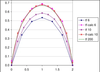
Figure 3: Normal thermal fluxes of the problem specified in (8) 0.0
0.1 0.2 0.3 0.4 0.5 0.6 0.7
0 0.5 1 1.5 2
In Figure 3 results are compared on one of the straight boundaries of the problem specified by Equation (8). Mesh of quad elements was used as 6×6, 10×10 and 200×200 elements. The corresponding fluxes are denoted in the legend of Figure 3 as “tf 6“, “tf 10“ and “tf 200“, respectively. Normal heat flux “tf 200” for 200×200 quad mesh can be already assumed as exact result, as was verified by a convergence analysis. Recalculated normal fluxes on 6×6 and 10×10 meshes are designated as “tf-cal 6” and “tf-cal 10”. It is seen that these recalculated fluxes do as good a job as a mesh of 200x200 and that their coincidence with the “exact” values is just excellent.
3.2 Stoke’s
domain
In the Stoke’s region the following scheme is used:
(
h) (
h h)
h h nh
Pˆ q ,
q w
,
q S
k
t = ∇⋅ ∀ ∈
Γ v ,
h n h n h
n v w v
~ = − . (9)
Here w is an auxiliary value of the normal velocity, used to correct the originally hn obtained normal velocities, v . Originally obtained velocity field is hn vh and the new normal velocities are designated as ~ . Equation (9) is similar to Equation (7), but vnh in this case the incompressibility condition is completely separated from the full weak formulation and treated separately.
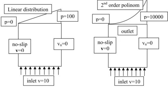
Efficiency of this technique, to our knowledge not yet published, was verified directly on ANSYS fluid element FLUID 141, where pressure and velocity components are nodal variables. Two test problems for unit viscosity and mass free fluid are specified in Figure 4, results of original and recalculated normal velocities are shown in Figures 5 and 6, respectively.
Figure 4: Two test fluid problems definitions p=0
inlet v=10 2ndorder polinom
vn=0
no-slip
v=0
p=10000 outlet
inlet v=10 p=0
p=100
vn=0
no-slip
v=0
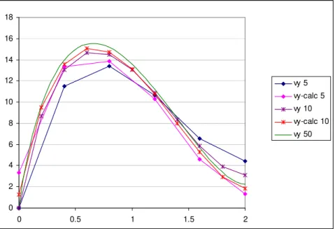
No units are stated in the test problems, because only relative comparison is important. Moreover pressure in these test problems does not correspond to the capillary pressure, because the aim is only to test the efficiency of such methodology. Also here meshes of quad elements were used, now as 5x5, 10x10 and 50x50. The 50x50 mesh results can be assumed as the “exact” solution. In the legend of Figures 5 and 6 original values of normal velocities are designated as “vy 5“, “vy 10“ and “vy 50“ on 5x5, 10x10 and 50x50 quad meshes, respectively, and the recalculated values are stated as “vy-calc 5“ and “vy-calc 10“.
Figure 5: Results of the first test fluid problem
Figure 6: Results of the second test fluid problem
It can be again verified that the recalculated outlet normal velocities on coarse meshes 5x5 and 10x10 fit the “exact” solution well.
-1500 -1000 -500 0 500 1000
0 0.5 1 1.5 2 vy 5
vy-calc 5 vy 10 vy-calc 10 vy 50 b)
0 2 4 6 8 10 12 14 16 18
0 0.5 1 1.5 2
In order to additionally support the scheme presented in Equation (9), it can be proven, that in one-dimensional even compressible case, this scheme will always produce the exact analytical result, no matter what number of elements is used. Let us assume for the sake of simplicity Stoke’s problem on the interval [0, 1] with uniform discretization to “m” linear elements. Compressibility function will be designated as g(x) and boundary conditions will be stated as v(x=0)=v~ , p(x=1)=0 p~ , 1 where v~ and 0 p~ are given values. Expressing the velocity v in the usual way, one 1
gets
∑
= + = m 1 i i i 0 0 h N v N v ~
v , where Ni, i=1,..,m stand for the shape functions and vi,
i=1,..,m for the nodal unknowns. Simple calculation permits to obtain the set of equations in the following form:
(
v v~)
g( )
xN dx 21
0 0
1− =
∫
,(
v ~v)
g( )
xNdx 21
1 0
2 − =
∫
,(
v v)
g( )
x N dx 21
2 1
3− =
∫
, ...(
v v)
g( )
x N dx2 1 1 m 2 m
m − − =
∫
− ,(10)
Having the solution in the following form:
( )
xN dx 2 g( )
xN dx ... g2 v ~
vm = 0 +
∫
m−1 +∫
m−3 + ,( )
x N dx 2 g( )
xN dx ... g2 v ~
vm−1 = 0+
∫
m−2 +∫
m−4 + . …(11)
In accordance with Equation (9) and by substitution of Equation (11) one can finally obtain:
( )
x N dx g( )
xN dx g( )
xN dx g( )
x N dx... gwh =−
∫
m +∫
m−1 −∫
m−2 +∫
m−3 ,( )
( )
( )
( )
x N dx v~ g( )
xdx g ... ... dx N x g dx N x g dx N x g v ~ v ~ 0 0 2 m 1 m m 0 h∫
∫
∫
∫
∫
+ = + + + + += − − (12)
which finalizes the proof.
4 Conclusion
to obtain stable and accurate answers and it also allows one to step through larger time steps during the impregnation process.
Acknowledgments
Firstly named author would like to thank to the Portuguese institution for founding research Fundação para a Ciência e a Tecnologia for the scholarship allowing developing this work.
References
[1] S.G. Advani, M.V. Bruschke, R.S. Parnas, “Resin transfer molding”, in “Flow and rheology in polymeric composites manufacturing”, Advani, S.G., (Editor), Elsevier Publishers, Amsterdam, 465-516, 1994.
[2] Z. Dimitrovová, S.G. Advani, “Mesolevel analysis of the transition region
formation and evolution during the liquid composite molding process”,
Computers & Structures, in press, 2004.
[3] R.S. Parnas, F.R. Phelan, “The effect of heterogeneous porous media on mold
filling in resin transfer molding“, SAMPE Quarterly, 22, 53-60,1991.
[4] R.S. Parnas, A.J. Salem, T.A.K. Sadiq, H.P. Wang, S.G. Advani, “The
interaction between micro- and macroscopic flow in RTM preforms“,
Composite Structures, 27, 93-107, 1994.
[5] T.A.K. Sadiq, S.G. Advani, R.S. Parnas, “Experimental investigation of
transverse flow through aligned cylinders“, International Journal of
Multiphase Flow, 21, 755-774, 1995.
[6] M.A.A. Spaid, F.R. Phelan, “Modeling void formation dynamics in fibrous
porous media with the Lattice Boltzman method“, Composites A, 29A,
749-755, 1998.
[7] Z. Dimitrovová, S.G. Advani, “Free boundary viscous flows at micro and mesolevel during liquid composites molding process”, in “CD of communications of the 14th International Conference on Composites Materials”, San Diego, California, EUA, 2003.
[8] K. Potter, “Resin transfer molding”, Chapman & Hall, London. 1997.
[9] N. Patel, L.J. Lee, “Effects of fiber mat architecture on void formation and
removal in liquid composite molding“, Polymer Composites, 16, 386-399,
1995.
[10] N. Patel, V. Rohatgi, L.J. Lee, “Micro scale flow behavior and void formation mechanism during impregnation through a unidirectional stitched
fiberglass mat“, Polymer Engineering and Science, 35, 837-851, 1995.
[11] C. Binetruy, B. Hilaire, J. Pabiot, “The influence of fiber wetting in resin
transfer molding: scale effects“, Polymer Composites, 24, 548-557, 2000.
and Applications”, Hartland, S., (Editor), Surfactant Science Series, 119, Marcel Dekker, Inc., New York, Chapter 5, 263-312, 2004.
[13] Z. Dimitrovová, S.G. Advani, “Analysis and characterization of relative permeability and capillary pressure for free surface flow of a viscous fluid
across an array of aligned cylindrical fibers”, Journal of Colloid and
Interface Science, 245, 325-337, 2002.
[14] Z. Dimitrovová, S.G. Advani, “Numerical simulation of free boundary viscous flows at all length scales of LCM process”, in “CD of communications of the 3th International Conference on Computational & Experimental Engineering and Sciences”, Corfu, Greece, 2003.
[15] T.J.R. Hughes, G. Engel, L. Mazzei, M.G. Larson, “The continuous Galerkin
method is locally conservative”, Journal of Computational Physics, 163,
467-488, 2000.
[16] I. Babuška, A. Miller, “The post-processing approach in the finite element method - Part 1: Calculation of displacements, stresses and other higher
derivatives of the displacements”, International Journal for Numerical