Abstract
Post-processing a finite element solution is a well-known technique, which consists in a recalculation of the originally obtained quantities such that the rate of convergence increases without the need for expensive remeshing techniques. Post-processing is especially effective in problems where better accuracy is required for derivatives of nodal variables in regions where Dirichlet essential boundary condition is imposed strongly. Consequently such an approach can be exceptionally good in modelling of resin infiltration under quasi steady-state assumption by re-meshing techniques and with explicit time integration, because only the free-front normal velocities are necessary to advance the resin front to the next position. The new contribution is the post-processing analysis and implementation of the free-boundary velocities of mesolevel infiltration analysis. Such implementation ensures better accuracy on even coarser meshes, which in consequence reduces the computational time also by the possibility of employing larger time steps.
Keywords: post-processing techniques, Darcy flow, Stokes flow, free boundary
flows, mesolevel analysis, capillary pressure, liquid composite moulding.
1 Introduction
New trends in transportation industry ask for implementation of fibre reinforced composites, because of their design versatility, low weight, high mechanical performance tailorable to the industrial requirements, resistance to the environmental conditions, net shape and sometimes possibility of an easy repair and/or recycling. Structural pieces fabricated by pre-preg technology are being replaced by components manufactured by recent methodologies called Liquid composite moulding processes (LCM). Among them, Resin transfer moulding (RTM), Vacuum assisted resin transfer moulding (VARTM) and Vacuum assisted resin infusion (VARI), belong to the group of low injection pressure processing
Post-processing Techniques in Free Boundary Flows
during Liquid Composite Moulding Processes
Z. Dimitrovová
UNIC, Department of Civil Engineering
New University, Monte de Caparica, Portugal
techniques. When large products in smaller series are required, demands on further cost reduction, which can be achieved either by cycle time decrease or moulds manufacturing cost reduction, are becoming crucial. Then VARTM and VARI, happen to be more attractive, as they require only one rigid mould face and can be processed under room temperature. Physics of the resin advance and thickness variation in these technologies is not yet fully understood and therefore the risk of failure during production of large pieces is still considered too high.
Reliable flow simulation software is inevitable in determination of an optimal injection strategy. Available simulation software is usually based on Darcy’s law, suited for macrolevel analysis and capillary action is either omitted or not accounted for correctly. Void formation during the injection phase can be explained as a consequence of the non-uniformity of the flow front progression. Origin of this fact lies in the dual porosity of the fibre preform and therefore the best explanation can be provided by mesolevel analysis. In the mesolevel analysis, single scale porous media (fibre tows) and open spaces are presented in the flow domain and therefore different flow regimes must be considered and linked together in one analysis, at each time step. In such simulation it is extremely important to account correctly for the surface tension effects, which can be modelled as capillary pressure applied at the flow front, [1].
Numerical techniques to address the movement of the flow were already developed in the Free Boundary Program (FBP) [2-4]. Numerical simulations can track the advancement of the resin front promoted by both hydrodynamic pressure gradient and capillary action. Base analysis is solved in commercial code ANSYS. However, capillary action implementation brings numerical difficulties, when continuous Galerkin method is used. This can be overcome by post-processing free-boundary normal velocities yielding superior convergence results. Post-processing a finite element solution is a well-known technique [5-9], which consists in a recalculation of the originally obtained quantities such that the rate of convergence increases without the need for expensive remeshing techniques. Post-processing methods are especially effective in problems where better accuracy is required for derivatives of nodal variables in regions where Dirichlet essential boundary condition is imposed strongly. The recalculation exploits the previous finite element solution and makes use of the space of trial shape functions that were omitted in the original formulation. Consequently such an approach can be exceptionally good in modelling of resin infiltration under quasi steady-state assumption by re-meshing techniques and with explicit time integration, because only the free-boundary normal velocities are necessary to advance the resin front to the next position.
published in [5-9] can be implemented, although in our case the problem must be posed differently, as explained further. For Stokes flow new technique is suggested, presented in its preliminary form in [10-11]. Both techniques still required considerable programming effort to be implemented in FBP. Several numerical examples discuss the details of implementation, benefits of post-processing, particular problems related to infiltration, namely singularities, corner problem and discontinuity in permeability, among others.
2 Mesolevel analysis
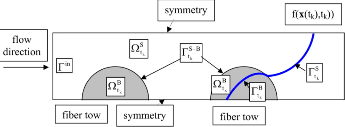
In mesolevel analysis, liquid flowing along two different scales must be considered and linked together. Single scale porous media, fibre tows, (shown in Figure 2 by grey half-circles) and open spaces (white spaces), implying different flow regimes during infiltration, are presented together in the flow domain. Fibre tows have uniformly distributed pores, therefore sharp flow front can be assumed as the resin impregnates. As the flow is slow, inertia terms can be neglected, thus one can assume Stokes flow in the currently filled inter-tow spaces St
k
Ω (white space between Γin and tS
k
Γ ) and Darcy flow in the saturated intra-tow region; Bt
k
Ω , which need to be coupled and solved at each discretized time tk. In fact, Darcy’s law must
be modified to Brinkman equations, in order to account for the viscous stress at the interface between these two regions ( tS B
k
−
Γ ). Viscous stress rapidly decreases with the distance from S B
tk
− Γ .
Figure 1: Flow domain, regions and boundaries designation. In summary, the following equations must be satisfied at each time step, tk:
in inter-tow spaces: ∇⋅v=0 and ∇p=μΔv in S tk
Ω
(Stokes equations), (1)
in intra-tow spaces: ∇⋅vD =0 and ∇pf =μΔvD−μK−1⋅vD in Bt
k
Ω
(Brinkman equations), (2)
fiber tow
symmetry flow
direction
fiber tow
in
Γ
S tk
Ω
B tk
Ω
B S tk
−
Γ
B tk
Γ
S tk
Γ
symmetry
B tk
Ω
where v is local velocity vector, p is local pressure, μ is resin viscosity and ∇ stands for spatial gradient, Δ=∇⋅∇. vD is Darcy velocity vector, i.e. the phase averaged velocity related to the intrinsic phase average vf by vD=φtvf, where φt is intra-tow
porosity. pf stands for intrinsic phase average of the local pressure and K is absolute permeability tensor.
If fibres inside the tows are rigid, impermeable and stationary, the following boundary conditions, under usual omission of the air pressure, must be fulfilled at the free front:
0 σv =
t and
(
)
p p p pc 2 Hv n
v⋅ ⋅ − =σ − ≈− =− =− γ
n n
σ at tS
k
Γ , (3)
pf=Pc at ΓtBk . (4)
Here σv is local viscous stress,σvt tangential vector component of the viscous stress vector, σvn normal component of the viscous stress and n is the outer unit normal vector to the free front in Stokes region tS
k
Γ . pc and Pc stand for local and global
(homogenized) capillary pressure, γ is the resin surface tension and H is the mean curvature. Progression of the free boundary can be determined according to:
0 f t
f Dt Df
= ∇ ⋅ + ∂ ∂
= v at S
tk
Γ , (5)
0 f t
f Dt Df
t D
= ∇ ⋅ φ + ∂ ∂
= v at tB
k
Γ , (6)
where f(x(t),t)=0 is implicit function describing the moving sharp flow front (dark bold line in Figure 1), x is spatial variable and t is time. Other boundary conditions such as symmetry, periodicity and inlet conditions at Γin are related to the particular problem under consideration.
3 Numerical simulation
Post-processing a finite element solution is a well-known technique, which consists in a recalculation of the originally obtained quantities such that the rate of convergence increases without the need for expensive remeshing techniques. Post-processing is especially effective in problems where better accuracy is required for derivatives of nodal variables in regions where Dirichlet essential boundary condition is imposed strongly. For Darcy flow analogy with thermal analysis can be exploited and technique already published in [5-9] can be implemented. Nevertheless in our case the problem must be posed differently, as explained in next section, with the help of several numerical examples. For Stokes flow new technique, presented in its preliminary form in [10-11], is suggested. Post-processing implementation ensure free boundary velocities of sufficient precision even from coarse meshes, which can significantly reduce CPU time. Time loss required for recalculation is completely equilibrated by the fact that this way the new free front shape is more exact, smoother and consequently larger time steps will be possible to implement. In summary, post-processing implementation ensure faster calculation without the danger of free boundary oscillation.
3.1 Post-processing of Darcy flow
In the region where Darcy flow is fully developed, normal component velocities on free boundary, where homogenized capillary pressure is imposed, can be recalculated from the following weak formulation [5-9]:
(
D,h)
(
h f,h) ( )
h h h nh
Pˆ q q
L p , q B v
~ ,
q B
k
t = − ∀ ∈
Γ , (7)
where B and L stand for bi-linear and linear form of the weak formulation. Recalculated components D,h
n
v
~ have superior convergence properties, in terms specified in [6]. Space of trial functions Pˆ includes now only the ones, which h where omitted from the previous formulation due to the essential boundary condition imposed on tB
k
Γ . Right hand side of Equation (7) can be calculated directly from the original solution pf,h; left hand side of the same equation require only integration along the free boundary, thus the new values can be obtained as a part of post-processing.
For Darcy flow analogy with thermal analysis can be exploited, thus pressure can be substituted by the temperature, θ, and Darcy velocity by the heat flux. In the literature, efficiency of technique (7) is usually shown on simple problem, which has analytical solution, like for instance:
(
1 x) (
21 y)
in[ ] [ ]
1,1 1,12 − 2 + − 2 − × −
= θ
Δ , (8)
[ ] [ ]
(
1,1 1,1)
on
0 ∂ − × − =
θ , (9)
(
2)(
2)
y 1 x
1− −
− =
θ (10)
and therefore the heat flux on the horizontal square sides is:
(
2)
1
y 21 x
/
y =± −
∂ θ ∂
±
= (11)
and analogous relation holds for the vertical sides.
When uniform mesh of square hхh elements is used, then the coefficients matrix on the left hand side of (7) is tri-diagonal, numbers on the main diagonal are 2h/3 surrounded by h/6. If the nodes numbering follows the boundary in one direction, then there is only one perturbation of this tri-diagonal property, in the first and the last line. Values on the right hand side of (7) correspond to integration over two adjacent elements, except of the square corners, where the trial function has support only over the corner element. Using the symmetry, equations related only to one side of the square domain can be extracted and solved. Then in the first and the last line the term on the main diagonal keeps its value 2h/3, and the neighbouring term is h/3. Recalculated flux has very good convergence properties, although the external normal is not defined in the corner. Results are shown in Figure 2.
0.0 0.5 1.0 1.5 2.0 2.5
-1 -0.8 -0.6 -0.4 -0.2 0 0.2 0.4 0.6 0.8 1
anal
tf2
tf2_rs
tf3
tf3_rs
tf4
tf4_rs
tf5
tf5_rs
tf6 tf6_rs
Figure 2: Original and recalculated heat flux on one side of the square domain of problem (8-9).
assumed purely mathematically, without physical meaning. Only linear elements are used in further discussions, for the sake of simplicity.
As can be seen in Figure 2, results are excellent and already for 6х6 mesh the maximum relative error is only 1.37%. In this comparison corners were excluded, because the analytical solution there is zero. In the corners the recalculated values are different from zero, on the contrary to the analytical and the original numerical solutions, but these differences look insignificant, due to the scale. If only one side of the square would be used for recalculation without the symmetry implementation, then the coefficients in the left hand side matrix in the first and the last line would be h/3 and h/6, and the recalculated solution would exhibit intolerable perturbation in the corners (Figure 3a). Implementing the technique suggested in [7], values in the corners are estimated by zero and the recalculated solution goes back to the previous nice form, but now with the exact value in the corners (Figure 3b). The legend keeps the same rules, “m” expresses that the recalculation technique was modified according to [7].
0.0 0.5 1.0 1.5 2.0 2.5
-1 -0.8 -0.6 -0.4 -0.2 0 0.2 0.4 0.6 0.8 1
anal tf2 tf2_r tf3 tf3_r tf4 tf4_r tf5 tf5_r tf6 tf6_r
0.0 0.5 1.0 1.5 2.0 2.5
-1 -0.8 -0.6 -0.4 -0.2 0 0.2 0.4 0.6 0.8 1
anal tf2 tf2_rm tf3 tf3_rm tf4 tf4_rm tf5 tf5_rm tf6 tf6_rm
Figure 3: (a) Recalculated heat flux without symmetry implementation, (b) recalculated heat flux with estimate according to [7].
For this simple problem integration was done exactly on maple. Good convergence properties were helped by the fact that the total heat generated in square, was underestimated for coarse meshes, thus as the mesh was getting finer, the “amount of load” was getting more accurate. In the next figure, the relative error in absolute value is plotted against logarithm of the element size. As already seen in Figures 2-3, original numerical solution is always bellow, and the recalculated values are always above the analytical curve. Also L2-norm of the absolute error is
included in Figure 4. Next, in Figure 5, log-log plot of L2-norm against element size
0.0 0.2 0.4 0.6 0.8 1.0 1.2 1.4
-0.5 -0.4 -0.3 -0.2 -0.1 0
L2_sol L2_rec err_sol err_rec heat vol
Figure 4: L2-norm, relative error and the error in imposed heat source (“heat vol”) as a function of logarithm of element size (“sol” stands for the original and “rec” for
the recalculated values).
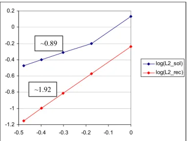
-1.2 -1 -0.8 -0.6 -0.4 -0.2 0 0.2
-0.5 -0.4 -0.3 -0.2 -0.1 0
log(L2_sol) log(L2_rec)
Figure 5: Log-log plot of L2-norm against element size for original (“sol”) and
recalculated (“rec”) solution.
It is necessary to point out, that these “classical” problems do not correspond to the real situation of resin infiltration, and therefore do not serve for the technique efficiency confirmation for infiltration task. In the analogous problem there is no heat source, but usually heat flux is imposed on one side of the domain (inlet) and temperature is prescribed at the other side (outlet). In terms of Darcy infiltration: inlet flow rate is prescribed and at the outlet pressure is imposed to simulate the surface tension effect. Remaining boundaries are submitted to Neumann homogeneous condition. Therefore, it is necessary to justify post-processing efficiency on problems like:
~0.89
[ ] [ ]
1,1 1,1 in0 − × − =
θ
Δ , 0 onx 1andy
[ ]
1,1n = =± ∈ −
∂ θ ∂
,
[ ]
1,1 xand 1 y for 10
n =− =− ∈ −
∂ θ ∂
, θ
( )
x =θ0( )
x for y=1andx∈ −1,1 .(12)
It is shown firstly, that when function representing the Dirichlet condition, θ0
( )
x , does not belong to C1 and does not have zero side derivatives at ±1, i.e. when the Dirichlet condition causes singularity of the heat flux at the outlet, post-processing does not really helps and suggestions from [7] are not also very useful. Then smooth function is chosen to justify the effectiveness and finally discontinuity in permeability is analyzed. Two cases were chosen to demonstrate singularities:( )
x 100(
1 x)
0 = −
θ (case 1), θ0
( )
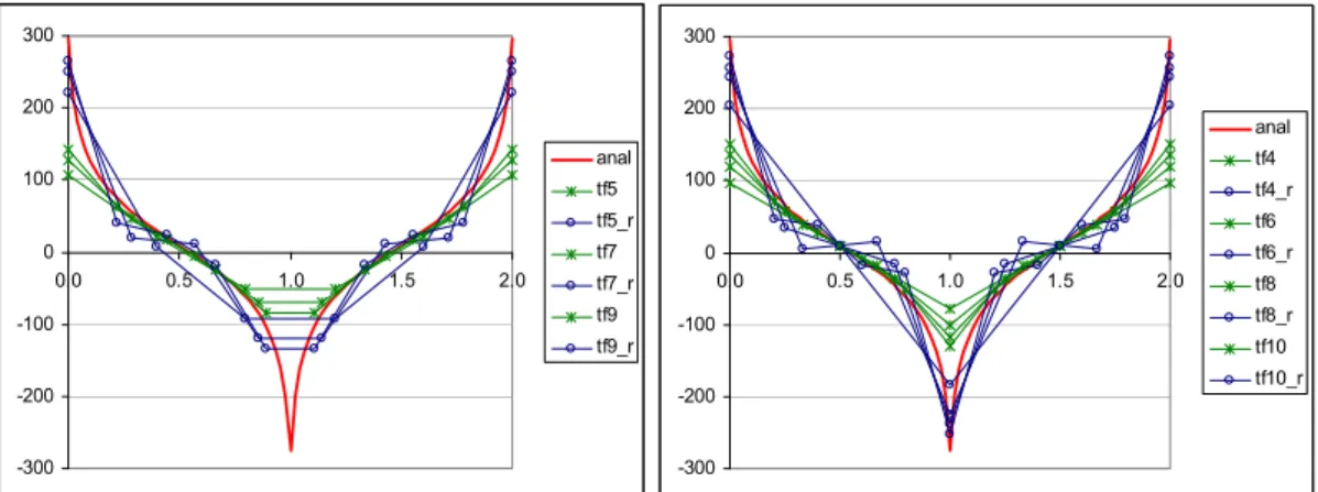
x =100x2 (case 2). (13)In the first case the imposed function is piece-wise linear, and causes singularities in the middle and at ±1, in the second case quadratic function was chosen, and only side singularities occur. Results are separated to even and odd divisions of the square domain. Analytical solution was approximated by numerical results from 200х200 mesh. Results from case 1 are summarized in Figure 6, legend obeys the same rules as in Figures 2-3.
-300 -200 -100 0 100 200 300
0.0 0.5 1.0 1.5 2.0 anal tf5 tf5_r tf7 tf7_r tf9 tf9_r
-300 -200 -100 0 100 200 300
0.0 0.5 1.0 1.5 2.0 anal tf4 tf4_r tf6 tf6_r tf8 tf8_r tf10 tf10_r
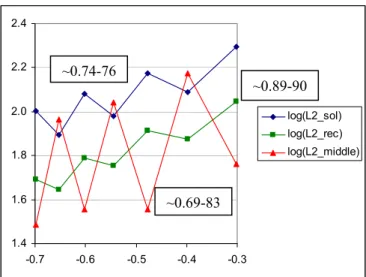
1.4 1.6 1.8 2.0 2.2 2.4
-0.7 -0.6 -0.5 -0.4 -0.3
log(L2_sol) log(L2_rec) log(L2_middle)
Figure 7: Log-log plot of L2-norm against element size for original (“sol”),
recalculated (“rec”) and element side flux (“middle”) solution of problem (12-13), case 1.
Also in case 2 oscillation of the recalculated values was observed (Figure 8). As singularity takes place only in the corner, at first, suggestions from [7] were implemented. In this particular case, corner value estimate is not possible to implement, therefore it is suggested that as much as exact value should be used instead. The exact value is actually minus infinity, but when this value was introduced into the equations to be solved, then for even number of divisions, recalculated values were completely out of sense. By substitution of some sufficiently large value oscillation was not removed and moreover outlet flux conservation was violated. For the sake of comparison absolute error (in absolute value) is compared in Figure 10, plotted against logarithm of number of divisions.
-500 -400 -300 -200 -100 0 100 200
0.0 0.5 1.0 1.5 2.0 anal tf5_r tf7_r tf9_r
-500 -400 -300 -200 -100 0 100 200
0.0 0.5 1.0 1.5 2.0 anal tf4_r tf6_r tf8_r tf10_r
Figure 8: Original and recalculated heat flux of problem (12-13), case 2. ~0.74-76
~0.89-90
-300 -250 -200 -150 -100 -50 0 50 100 150
0.0 0.5 1.0 1.5 2.0 anal tf5 tf5_re tf7 tf7_re tf9 tf9_re
-300 -250 -200 -150 -100 -50 0 50 100 150
0.0 0.5 1.0 1.5 2.0 anal tf4 tf4_re tf6 tf6_re tf8 tf8_re tf10 tf10_re
Figure 9: Original heat flux and recalculated element side flux (“re”) of problem (12-13), case 2.
0 100 200 300 400 500
0.6 0.7 0.8 0.9 1 sol rec middle
0 20 40 60 80
0.6 0.7 0.8 0.9 1 sol rec middle
Figure 10: Maximum absolute error comparison for original (“sol”), recalculated (“rec”) and element side flux (“middle”) solution of problem (12-13), case 2, with
corner values included (left) and excluded (right).
1.6 1.8 2.0 2.2 2.4 2.6
-0.7 -0.6 -0.5 -0.4 -0.3
log(L2_sol)
log(L2_rec)
log(L2_middle)
Figure 11: Log-log plot of L2-norm against element size for original (“sol”),
recalculated (“rec”) and element side flux (“middle”) solution of problem (12-13), case 2.
~0,72
~1,01
On the contrary to case 1, in case 2 convergence was also helped by the fact, that with finer mesh, function θ0
( )
x was imposed more accurately. Nevertheless it was demonstrated that the post-processing recalculation did not improve the convergence significantly when the function θ0( )
x was not smooth enough. By implementing element side flux, the convergence got even worse than for the original solution.As infiltration problem has a physical base, one is allowed as to assume, that capillary pressure can be estimated by sufficiently smooth function, namely by function from C1. If moreover extension of the problem would be possible by symmetry or periodicity, also side derivatives at ±1 would be zero, and there would be obviously no corner problem and no singularities. To analyze such situation, function of the form:
( )
⎟⎠ ⎞ ⎜ ⎝ ⎛ π =
θ x
2 sin 100 x
0 , (14)
was chosen. Results are shown in Figures 12-14.
-200 -100 0 100 200
0.0 0.5 1.0 1.5 2.0 anal tf3 tf3_re tf5 tf5_re tf7 tf7_re tf9 tf9_re
-200 -100 0 100 200
0.0 0.5 1.0 1.5 2.0 anal tf2 tf2_re tf4 tf4_re tf6 tf6_re tf8 tf8_re tf10 tf10_re
Figure 12: Original and recalculated element side flux of problem (12, 14).
0 10 20 30 40 50 60 70
0.2 0.4 0.6 0.8 1 sol rec middle
0 5 10 15 20 25 30 35
0.2 0.4 0.6 0.8 1 sol rec middle
Figure 13: Maximum absolute error comparison for original (“sol”), recalculated (“rec”) and element side flux (“middle”) solution of problem (12, 14), with corner
Excluding singularities, post-processed values recovered excellent properties like in problem (8-9), on 10х10 mesh maximum relative error is only 2.1% and 0.66% for the element side flux. However when L2-norm on log-log plot is compared, it is
seen in Figure 14, that the element side flux recalculation can have some unexpected perturbations. Slope is improved from 0.64 to 1.56, which is more than sufficient and the option with element side flux can be refused as unreliable.
-1.5 -1.0 -0.5 0.0 0.5 1.0 1.5 2.0
-0.8 -0.6 -0.4 -0.2 0
log(L2_sol) log(L2_rec)
log(L2_middle)
Figure 14: Log-log plot of L2-norm against element size for original (“sol”),
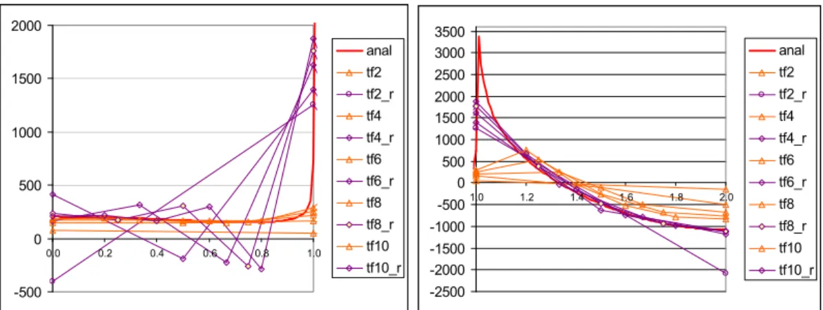
recalculated (“rec”) and element side flux (“middle”) solution of problem (12, 14). Same results were obtained for the original (not analogous) analysis by Flotran (ANSYS CFD module) using linear square fluid elements. Another important problem, which must be analyzed, is how to treat a discontinuity in permeability. Due to small pores between fiber tows, Stokes flow in free spaces could be sometimes approximated by Darcy flow in very high permeability region. When discontinuity in permeability (thermal conductivity in analogous problem) is implemented, there is a difference between the fluid and the analogous thermal solution. Thermal solution has discontinuity in the heat flux along the line of change while in Flotran solution velocity is kept as continuous. In fact, sudden change in the velocity must occur and this would be very difficult to model on coarse mesh, even with the help of post-processing. The test problem chosen for this analysis is the same as (12, 14), only on the right hand side of the fluid flow square domain, permeability (or thermal conductivity) is ten times higher than on the left hand side. Firstly, the problem was studied in Flotran. After recalculation no improvement was obtained as can be seen in Figures 15-16. This is caused by the coarse mesh and continuous velocity value in the region, where sudden change is expected. Recalculation was modified by imposed discontinuity, but results were not improved. Therefore analogous problem was examined, where the discontinuity naturally comes from the solution. Recalculation had to be separated into two parts due to the discontinuity. Although the convergence was significantly improved as it is seen from Figure 18, slope of 0.68 was improved to 1.04, recalculated values distribution is not satisfactory.
~0.64
-500 0 500 1000 1500 2000
0.0 0.2 0.4 0.6 0.8 1.0
anal tf2 tf2_r tf4 tf4_r tf6 tf6_r tf8 tf8_r tf10 tf10_r -2500 -2000 -1500 -1000 -500 0 500 1000 1500 2000 2500 3000 3500
1.0 1.2 1.4 1.6 1.8 2.0
anal tf2 tf2_r tf4 tf4_r tf6 tf6_r tf8 tf8_r tf10 tf10_r
Figure 15: Original and recalculated velocities of discontinuity test problem solved by Flotran on the left (left) and right (right) part of the domain.
2.30 2.40 2.50 2.60 2.70 2.80 2.90
-0.8 -0.6 -0.4 -0.2 0
log(L2_sol)
log(L2_rec)
log(L2_middle)
Figure 16: Log-log plot of L2-norm against element size for original (“sol”),
recalculated (“rec”) and element side flux (“middle”) solution of discontinuity test problem solved by Flotran.
-300 -200 -100 0 100 200 300 400
0.0 0.2 0.4 0.6 0.8 1.0
anal tf2_r tf4_r tf6_r tf8_r tf10_r -2500 -2000 -1500 -1000 -500 0 500 1000 1500 2000 2500 3000 3500
1.0 1.2 1.4 1.6 1.8 2.0
anal tf2_r tf4_r tf6_r tf8_r tf10_r
2.40 2.60 2.80 3.00 3.20 3.40
-0.8 -0.6 -0.4 -0.2 0
log(L2_sol) log(L2_rec) log(L2_middle)
Figure 18: Log-log plot of L2-norm against element size for original (“sol”),
recalculated (“rec”) and element side flux (“middle”) solution of discontinuity test analogous problem.
In order to improve recalculated values distribution, “corner” influence was included in the following way: expected discontinuity of 10 was prescribed on vertical heat flux and another unknown, the corner flux horizontal value was implemented and solved. Any other option would lead to outlet flux violation. Convergence properties were maintained and distribution was improved significantly as shown in Figure 19.
-300 -200 -100 0 100 200 300 400
0.0 0.2 0.4 0.6 0.8 1.0
anal tf2_r
tf4_r tf6_r
tf8_r tf10_r
-2500 -2000 -1500 -1000 -500 0 500 1000 1500 2000 2500 3000 3500
1.0 1.2 1.4 1.6 1.8 2.0
anal tf2_r
tf4_r tf6_r tf8_r
tf10_r
Figure 19: Original and modified recalculated velocities of discontinuity test analogous problem on the left (left) and right (right) part of the domain.
In summary, for Darcy flow, post-processing can be used, it highly improves accuracy and convergence, but special attention must be paid to the capillary pressure estimation, only smooth functions from C1 with zero side derivatives must be used. Additional treatment must be included when next free front is established in the point of permeability discontinuity.
0.68
3.1 Post-processing of Stoke flow
The methodology implemented in Stokes region uses the following scheme, [10-11]:
(
h) (
h h)
h hn h Pˆ q , q w , q S k
t = ∇⋅ ∀ ∈
Γ v ,
h n h n h
n v w
v
~ = − , (15)
where w is an auxiliary value, which is used for the correction of the originally hn calculated velocities, v . Equation (15) is similar to Equation (7), but in this case hn incompressible condition is completely separated from the weak formulation of Stokes problem. It is proven in [10] that in one-dimensional case such recalculation leads an analytical value. Efficiency of the technique (15) can be shown on problem similar to (12, 14), which can be written as:
0 = ⋅
∇ v e ∇p=μΔv in
[ ] [ ]
−1,1× −1,1 , vx =0 forx=±1andy∈[ ]
−1,1[ ]
1,1 x and 1 y for 10vy = =− ∈ − , p
( )
x =p0( )
x fory=1andx∈ −1,1 ,( )
⎟ ⎠ ⎞ ⎜ ⎝ ⎛ π = x 2 sin 100 x p0 (16)Recalculated values have excellent properties as shown in Figure 20, on 10х10 mesh maximum relative error is only 1,05%.
-40 -20 0 20 40 60
0.0 0.5 1.0 1.5 2.0 anal uy3 uy3_r uy5 uy5_r uy7 uy7_r uy9 uy9_r -40 -20 0 20 40 60
0.0 0.5 1.0 1.5 2.0 anal uy2 uy2_r uy4 uy4_r uy6 uy6_r uy8 uy8_r uy10 uy10_r
Figure 20: Original and recalculated velocities of problem (16-17).
0 5 10 15 20 25 30 35
0.2 0.4 0.6 0.8 1 sol rec middle
0 2 4 6 8 10
0.2 0.4 0.6 0.8 1 sol rec middle
Figure 21: Maximum absolute error comparison for original (“sol”), recalculated (“rec”) and element side velocity (“middle”) solution of problem (16-17), with
corner values included (left) and excluded (right).
4 Conclusion
In this paper two techniques for post-processing a finite element solution are presented and tested on several examples, in order to evaluate their efficiency in infiltration problems on mesoscopic level of liquid composite moulding. For Darcy flow analogy with thermal analysis can be exploited and technique already published in [5-9] can be implemented. For Stokes flow new technique, presented in its preliminary form in [10-11], is suggested. Both techniques showed satisfactory properties and can significantly improve convergence slope in log-log plots. Special attention must be paid to the capillary pressure estimation in order to prevent unphysical boundary oscillation. Additional care must be taken when next free front is established in the point of permeability discontinuity. Post-processing implementation ensure free boundary velocities of sufficient precision even from coarse meshes, which can significantly reduce CPU time. Time loss required for recalculation is completely equilibrated by the fact that this way the new free front shape is more exact, smoother and consequently larger time steps will be possible to implement. In summary, post-processing implementation ensure faster calculation without the danger of free boundary oscillation.
References
[1] S.G. Advani, Z. Dimitrovová, “Role of Capillary Driven Flow in Composite Manufacturing”, in Surface and Interfacial Tension: Measurement, Theory and Applications, ed. S. Hartland, Surfactant Science Series, 119, 263-312, 2004, Marcel Dekker, Inc., NY.
[3] Z. Dimitrovová, S.G. Advani, “Free boundary viscous flows at micro and mesolevel during liquid composites molding process”, International Journal for Numerical Methods in Fluids, 46, 435-455, 2004.
[4] Z. Dimitrovová, S.G. Advani, “Mesolevel analysis of the transition region formation and evolution during the liquid composite molding process”, Computers & Structures, 82, 1333-1347, 2004.
[5] G.F. Carey, “Derivative calculation from finite element solution”, Computer Methods in Applied Mechanics and Engineering, 35, 1-14, 1982.
[6] I. Babuška, A. Miller, “The post-processing approach in the finite element method - Part 1: Calculation of displacements, stresses and other higher derivatives of the displacements”, International Journal for Numerical Methods in Engineering, 20, 1085-1109, 1984.
[7] G.F. Carey, S.S. Chow, M.K. Seager, “Approximate boundary-flux calculations”, Computer Methods in Applied Mechanics and Engineering, 50, 107-120, 1985.
[8] A. Mizukami, “A mixed finite element method for boundary flux calculations”, Computer Methods in Applied Mechanics and Engineering, 57, 239-243, 1986.
[9] T.J.R. Hughes, G. Engel, L. Mazzei, M.G. Larson, “The continuous Galerkin method is locally conservative”, Journal of Computational Physics, 163, 467-488, 2000.
[10] Z. Dimitrovová, S.G. Advani, “Numerical Method to Predict Void Formation during The Liquid Composite Molding Process”, 7th International Conference on Flow Processes in Composite Materials, Newark, Delaware, EUA, July, 2004, 269-274, 2004.