ISSN 2179-8087 (online)
Original Article
Conservation of Nature
Creative Commons License. All the contents of this journal, except where otherwise noted, is licensed under a Creative Commons Attribution License.
Simulation of Flow in the Capim River (PA) using the
SWAT Model
Hildo Giuseppe Garcia Caldas Nunes
1
, Adriano Marlisom Leão de Sousa
1
,
Joyse Tatiane Souza dos Santos
2
1Instituto Sócioambiental e dos Recursos Hídricos, Universidade Federal Rural da Amazônia – UFRA, Belém/PA, Brasil 2Programa de Pós-graduação em Ciências Ambientais, Universidade Federal do Pará – UFPA, Belém/PA, Brasil
ABSTRACT
Flow in the Capim River watershed, located in the state of Pará, Brazil, was estimated using the Soil and Water Assessment Tool (SWAT) model in order to determine its use efficiency. The meteorological data (from 2000 to 2010) were collected from an automatic station located in the municipality of Paragominas. The pluviometric and fluviometric data are available at the National Water Agency (ANA) website. Overall results show Efficiency Coefficient (Eff ) values of 0.65 (for sub-basin 5) and 0.87 for the entire investigated period. The results also show a reduction in Eff estimation error, which started from over-estimation of 219.18% and declined to underestimation of 18% (in sub-basin 5). In summary, validation of the SWAT model was successful after adjusting the sensors during the calibration phase. Thereby, this model can be used in other studies evaluating river basins.
1. INTRODUCTION
Since the 1980’s, several hydrometeorological studies have been conducted in basins located in tropical regions in Brazil in an attempt to understand, quantitatively and qualitatively, the processes involved in the hydrological and biogeochemical cycle of the watersheds (Sousa et al., 2010; Souza & Oyama, 2011). These studies sought to understand the effects of climate change on upland forests in Amazonia. Similarly, other projects, such as the ARME (Amazonian Region Micrometeorological Experiment) (Shuttleworth, 1988), GTE/ABLE (Global Tropospheric Experiment/Amazon Boundary Layer Experiment) (Garstang et al., 1990), ABRACOS (Anglo-Brazilian Amazonian Climate Observation Study) (Shuttleworth et al., 1991; Gash et al., 1996) and LBA (Large Scale Biosphere-Atmosphere Experiment in Amazonia) (Marengo et al., 2012), have also invested in research and field experiments aiming to answer questions related to the same theme.
Thereby, the use of hydrological models has become a great ally of these studies, as it has provided better understanding of the processes that involve the hydrological cycle of watersheds. Thus, they enable better practices and land occupation and management that make permanence and maintenance of ecosystems possible (Abbaspour et al., 2006).
Hydrological cycle components (flow, precipitation, amount of water into the soil, surface runoff, total water production reaching the channel, underground flow, percolation, actual and potential evapotranspiration) influence different aspects of human life, namely, agricultural yield, energy generation, flood control, water production to industry and dwellings, flora and fauna management, etc. They are susceptible to changes originating from both natural (climatic variability) and anthropic causes (Tomasella et al., 2009).
Radiative surface processes are important for the redistribution of heat into the soil and in the atmosphere. Together with the hydrological cycle, they are essential for climatic and hydrological modeling, and the magnitude of these components and their variations, in periods shorter than one day, are important for the parameterization and calibration of global circulation models. At longer intervals, these quantities are also used in models of global climatic impacts resulting from physiographic changes of the surface (Souza &
Oyama, 2011). The literature shows that the feedback hypotheses between soil moisture and precipitation are fundamental elements for establishing the behavior of the hydrological cycle. Eltahir (1998) states that the central point of this process is on the interface of the energy-to-surface balance.
Moreover, estimates of the spatial-temporal variation of surface heat fluxes and soil moisture would enable understanding of the evaporative processes, which are fundamental aspects in many applications that focus on water resources and climate modeling (Mohamed et al., 2004). However, due to the scarcity of meteorological data, atmospheric and hydrological models are often fed with regional data with inadequate resolution to represent the atmospheric conditions, which are to be modeled (Abbaspour et al., 2006).
Remote sensing associated with modelling, such as the SEBAL (Surface Energy Balance Algorithms for Land) (Allen et al., 2002) and METRIC (Mapping Evapotranspiration at High Resolution with Internalized Calibration) (Allen et al., 2007), have demonstrated great potential for attending the needs related to water balance computation, in regional scale or in watersheds. These tools are suitable for spatial information collection and their application implies considerable improvement in the assimilation of hydrological modeling, as well as in climate modeling, in order to generate future regional scenarios and possible impacts on climate and hydrology. As a consequence, models that represent the hydrological cycle can effectively contribute to the planning and management of water resources (Faramarzi et al., 2009; Sousa et al., 2015).
The SWAT model was chosen for this research because it is suitable for application in medium-sized basins (±30,000 km2), in addition to its quantitative
in the state of Pará, Brazil. The analysis begins from the evaluation of the agreement between estimated and observed flow values.
2. MATERIAL AND METHODS
2.1. Study area
This research was conducted in the Capim river basin, which is located in the northeast and west regions of Pará and Maranhão states, respectively. This watershed has an area of 37,199.22 km2 and covers
the municipalities of São Domingos do Capim, Aurora do Pará, Ipixuna do Pará, Paragominas, Goianésia do Pará, Dom Eliseu, Ulionópolis, and Rondon do Pará in Para state, and Açailândia, Cidelândia, and Vila Nova dos Martírios in Maranhao state. Climatic data were collected from an automatic weather station belonging to the National Institute of Meteorology (INMET) located in the municipality of Paragominas, Para state, whereas hydrological data (fluviometric and pluviometric) were provided by the National Water Agency (ANA) (Figure 1).
The Capim river basin was characterized considering the type, use and occupation, and slope of the soil. The predominant soil types in the watershed are Yellow Argisol, Yellow Latosol, Yellow-Red Latosol, and the Fluvic Neosol (IBGE, 2013). The basin is composed of 76% of Yellow Latosol (28,405.79 km2), approximately. The least representative soil is Red-Yellow Latosol (296.53 km2), comprising 0.8% of the basin area. Yellow Argisol (7,965.42 km2, approximately 21%) together with Yellow Latosol account for approximately 98% of the total area of the Capim River basin.
Yellow Argisol occurs in areas of flat relief, gently undulating, undulating, or even strongly undulating. The SWAT model soil database requires that physical characteristics of the soils in the basin be added. For more information, see the Brazilian Institute of Geography and Statistics (IBGE) (IBGE, 2013). Regarding land use and occupation in the Capim river basin, there are areas of forestry, agriculture, plant extractivism, farming, urban use, livestock, reforestation, environmental protection, and field (Venturieri et al., 2010).
As the manual of the Ecological-Economic Zoning of eastern and northern Pará state (ZEE-PA) considers the areas of plant extractivism as areas where wood extraction and/or forest seed exploration occur, the SWAT model considers these areas as forests (18,669.62 km2), and they represent 50.21% of the
total basin area.
The unclassified areas (portion of Maranhão State) were considered as livestock areas. Their proximity to this classification has been taken into account. These areas represent 28.46% of the basin, with 10,588.04 km2.
The watershed is composed of approximately 96% of forest, livestock, agriculture and environmental protection areas. The urban areas represent 0.07% of the total basin. They include an area of 26.64 km2,
which makes them the smallest land occupation in the basin. Regarding slope, the Capim river basin has altitudes varying from 2 m, in the north part, to 411 m, in the south part. Average elevation is approximately 114 m in the middle of the basin. Much of the Capim river watershed is slightly regular in the mid-filed depression. Its least prominent relief is located in the north region of the Guamá-Capim interfluvium, in the municipalities of São Domingos do Capim and São Miguel do Guamá.
2.2. The SWAT model
The initial step for the SWAT model operation occurs through the insertion of required information points (IPs). The IPs constitute the entry of data into grid points of the same geographical coordinate, with resolution and scale of 90 m and 1:300.00, respectively. The second IPs are performed using the ArcGis 9.3 software.
The parameters required by the SWAT model include climatic (INMET), use and type of soil (ZEE-PA and IBGE), and hydrological (ANA) data. This information depended on daily precipitation observations at four stations (São Domingos do Capim, Maringa, Paragominas, and Capim 2) (ANA); mean daily
observations of meteorological variables (precipitation, air temperature, relative humidity, solar radiation, and horizontal wind speed) at the Paragominas station; as well as on maps of soil type (IBGE), land use and occupation (ZEE-PA), and hydrography and topography (Digital Elevation Model (DEM)) (Table 1).
Data gaps (in the climatic and pluviometric series) were filled by the climatic generator CLIGEN, which reproduces daily series of time stochastically based on the monthly historical averages and the (statistical) parameters of a given geographic point; for more details see Caviglione (2013).
2.2.1. Parameter sensitivity
Abbaspour et al. (2006) affirmed that the SWAT model is sensitive to more than 100 variables associated with vegetation, land management, soil, climate, aquifer, channel, and reservoir. Once this analysis was performed automatically, all the parameters referring to the aforementioned variables were tested in this research. This is essential to answer questions such as “Where should data collection efforts be focused?”, “How much care should be taken in estimating the parameters?”, and “What is the relative importance of several parameters?”. The SWAT model presents an automatic parameter sensitivity analysis tool combining One-factor-at-a-Time (OFAT) and Latin Hypercube (LH) methods.
2.2.2. Calibration and validation
Calibration and validation are essential steps for the model efficiency. In order to calibrate and validate the model, two time series of real data of the basin under study are necessary. In the first stage (calibration), the most sensitive parameters in the basin are adjusted until the responses approach the observed values also based on the bibliographic search of the adjusted parameters. Through the first method (OFAT), the model promotes the change of only one parameter to each simulation. Thereby, the inserted changes are related to the altered parameter. In the second method (LH), the model is
Table 1. Data used in the study.
Data used Period Data gap (days) Consistency level
Climatic 2007 to 2010 65 Consisted
Pluviometric 2000 to 2010 225 Consisted
Soil type 2009 to 2010 - Consisted
based on the Monte-Carlo simulation (it generates observations with some probability distribution and the use of the obtained sample to approximate the function of interest), which eliminates the need for many simulations required through a stratified sampling method, enabling a robust estimation of the exit statistics; for more details see Faramarzi et al. (2009).
For validation, the results obtained for the two time series are compared using graphical methods such as hydrograms and regression lines, or analyses such as the Student’s t-test and the coefficient of efficiency (Eff) (Faramarzi et al., 2009). Calibration was performed by comparing the simulated flow values to the observed values for a period of seven years (January 2000 to December 2006). The validation of this work was conducted from January 2007 to December 2010.
2.2.3. Model efficiency assessment
Four methods were used to verify whether the measured values and those simulated by the SWAT model were with good adjustments:
Nash-Sutcliffe Efficiency Coefficient (Eff) (Nash & Sutcliffe, 1970), which represents the weighted variance of the events observed and calculated by the model. It varies from - ∞ to 1. The closer to 1, the closer to perfect the simulated event is. The Eff is expressed by equation 1: ( ) ( ) 2 1 2 1 1 n ob cal i n ob m i E E Eff E E = = − = − −
∑
∑
(1)Where: n, is the number of events; Eob, is the observed ,
event; Ecal, is the calculated event; and Em, is the average
of the observed event in the period.
Standard deviation (SD), in which the smaller the SD, the more perfect the adjustment of the simulated event in analysis related to the observed event. The SD is given by equation 2:
.1 00
ob cal ob E E SD E −
= (2)
Where: SD, is the standard deviation in %; Eob, is the
observed event for the period; and 0 Ecal, is the simulated
event for the same period.
Residual Mass Coefficient (RMC), which indicates when the model underestimates (positive) or
overestimates (negative) the output values. The RMC is given by equation 3:
1 1 1 n n ob cal i i n ob i E E RMC E = = = − =
∑
∑
∑
(3)Where: RMC, is the residual mass coefficient and n, is the number of events.
Mean Error (ME), in which the analyzed event is obtained by the quantitative difference between the simulated and observed events. and the ME is expressed by equation 4:
1 n cal ob i E E ME n = −
=
∑
(4)Where: n is the number of simulated events and EM is the mean error.
Based on these values, the result obtained by the SWAT model was used to simulate three experiments. The first experiment was conducted at initial conditions in order to evaluate the efficiency of the model in the generation of flow. In the second experiment, the manual calibration of the model was executed. Finally, in the third experiment, the validation of the model was performed (Faramarzi et al., 2009).
2.2.4. Hydrological simulations
In the first experiment, the “automatic” (default) option of the model was used, in which the parameters did not change values. This experiment served as a basis for the second (calibration) and third (validation) experiments because of its simplicity and efficiency in representing the initial conditions of the study region. After that, the automatic sensitivity analysis was performed by the SWAT. The limits of each parameter were maintained (automatic), showing which parameters should be changed and why.
In the second experiment, a manual calibration of some parameters of the model was performed based on the sensitivity analysis. Three attempts were made to adjust the parameters during manual calibration, which aimed to improve the monthly behavior of the flow rate. The moment at which the Eff reached values ≥0.50 was adopted as the stopping point of these attempts, starting with the third experiment.
verify how the SWAT model was able to assimilate the information extracted from the images of the use and change in the soil for the prognosis of the flow rate in the watershed. After each experiment, it was verified to what level the model was able to reproduce the observed flow rate using the statistical tools previously describe.
3. RESULTS AND DISCUSSION
After insertion of the maps of the study area into the Digital Terrain Model (DTM), use and occupation of the soil, and soil types, the model generated a basin with an area of 37,199.23 km2 (Figure 2), which is
a value close to the one manually generated by the ArcGis (37,179.08 km2). In order to define the number
of sub-basins, the value of critical origin area suggested by the model generated 11 sub-basins. An out-point was manually added into sub-basin 5 (844.73 km2) to
coincide with the point of the fluviometric station and be used in the flow rate comparison (simulated and observed); this sub-basin represents 2.27% of the watershed (Figure 2). Sub-basin 8 was the largest (8,370.65 km2),
representing approximately 23% of the watershed area. Sub-basin 2 was the smallest (457.61 km2), accounting
for only 1.23% of the basin area. The average area of the sub-basins was 3,391.75 km2.
Regarding the slope classes, the Capim river basin cover mostly regions of flat and regular surface (slope of 0-5%), which represents approximately 61% of the total area. Few areas (4% of the basin) have average slope (1530%). Thus the watershed shows little variation in slope, mostly between 0 and 15%, in approximately 96% of its area).
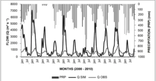
Climate data and soil physical characteristics were entered the model database and served as initial conditions for the model to fit the physical characteristics of the study area. Overall, the SWAT model simulated seasonality well, both qualitatively (efficiency analyzes) and quantitatively (overestimated total flow). However, the model behaved very inefficiently (Figure 3). Many authors have emphasized the difficulty of the SWAT in modeling baseline flow, because some parameters (default) referring mainly to the soil are not adequate for the basins located in Brazil (Sousa et al., 2015). The same was observed in this initial simulation. Using the initial conditions, results were very different from those observed; therefore, calibration should be performed before using this model in a watershed.
The SWAT model overestimated the peak flow rates for sub-basin 5 and underestimated the recession (quantitatively the model overestimated by 219.18% the total flow). This occurred because the model generates excessive baseflow and surface runoff. These results indicate that the model generated little evapotranspiration and that the amount of water in the soil was actually greater. It is noteworthy that the SWAT model also underestimated possible losses to the deep aquifer. Thereby, such conjuncture also influenced the recess of the curve over dry periods in sub-basin 5 (Figure 3).
Some advances could also be noticed in some of the model responses. This was probably due to the fact that sub-basin 5 is small. Considering that it presents a low time of concentration, the average precipitation verified
Figure 2. Capim river basin generated automatically by SWAT.
in one month may have generated a higher mean flow rate in the following month, which accelerated some peaks. However, regarding its curve of recession, the model managed to capture its seasonality. Even so, it has had some small peaks in these periods because the time of concentration in the sub-basin was low, as previously explained (Figure 3).
After identifying the most sensitive parameters and the points to be considered for the improvement and calibration of the hydrological simulation, we proceeded to choose the parameters that best fitted the search for solving the problems previously noticed. Some parameters were adjusted for sub-basin 5 (Table 2) in order to specifically reduce the total flow volume in the sub-basins and thus start the calibration step.
In the second experiment, in which manual calibration of the model was performed, the attempts to adjust the parameters aiming improvement of the initial results began with the selection of the three most sensitive parameters directly associated with volume reduction, with increase of the baseflow and adjustment of the recession curve. Namely, (Sousa et al., 2015): ALPHA_BF (baseflow recession parameter), CANMX (evapotranspiration increase), and SLOPE (increase of evapotranspiration, percolation, and baseflow), which were altered together with parameters regarding the soil; for more details on manual calibration, see in Abbaspour et al. (2006). Namely, GWQMN, GW_DELAY, SOL_AWC, and SHALLST (All these parameters were used to reduce the flow rate volume) (Table 3).
Table 2. List of parameters to be changed for each required adjustment and their causal relations with the respective settings for sub-basin 5.
Reduction of total flow volume Increase in baseflow and
recession curve Flow delay CANMX(+), CN2 (-), ESCO (-),
SLOPE (-), SOL_AWC (+), SLSUBBASIN (+),
SOL_K(-)
ALPHA_BF (+), GWQMN (-), GW_REVAP (+), RCHRG_DP (-),
REVAPMN (+)
LAT_TIME (+), SURLAG (-)
Where: CANMX (Maximum canopy storage); CN2 (Runoff curve number for moisture condition); ESCO (Soil evaporation compensation factor); SLOPE (Slope class simulated); SOL_AWC (Available water capacity of soil layer); SLSUBBASIN (Slope class of subbasin); and SOL_K (Saturated hydraulic conductivity of soil layer).
Table 3. Parameters modified in the manual calibration and their respective initial values in experiment 1.
MODIFIED PARAMETERS
Initial
Simulation MANUAL CALIBRATION
EXP. 1 CAL.1 CAL. 2 CAL. 3
GWQMN (mm) 2500 10 200 1000
GW_DELAY (day) 100 500 400 220
REVAPMN (mm) 1 500 50
ALPHA_BF 0.2 0.4 0.8 1.2
SOL_AWC (mm) 0.1 0.4 0.32
GW_REVAP 0.4 0.05 0.2
SHALLST (mm) 0.5 500
DEEPST 1000 1500
SURLAG 4 1
RCHRG_DP 0.3 1 0.2
SLOPE (m/m) var. 0.5 x var. 0.25 x var.
SLSUBBASIN var. 2 x var.
ESCO 2 1 0.237
CANMX (mm) 0 a 5 0 a 10
After the adjustments, the model overestimated the flow peaks in 2001 and 2004; underestimated the flow peaks 2000, 2003, and 2006; and no significant difference from the observed flow was found in 2005. With respect to the quantitative efficiency, the model showed good performance, with 93% response to the total observed and underestimation of 7% in the total flow rate. In comparison to the initial simulation, the adjustments reduced the monthly average volume by 3,000 m3s-1 in the peaks and adjusted the recession
period by 246 m3s-1. This shows and justifies large
improvements in the quantitative efficiency of the SWAT model (Figure 4).
Mean flow rate was 445.35 m3s-1, whereas the
observed rate for the period was 476.66 m3s-1. Some
delays were verified in the flow rate peaks in 2002 and 2003, which were essential for limiting the efficiency of the monthly flood simulations, as well as the poor simulation in 2006 (Figure 4).
As for the third experiment, which was the validation of the model, the SWAT model closely followed the seasonality of the mean flow rate in this sub-basin. It also showed its efficiency in simulating this event. It should be noted that in 2010, when the model did not follow the seasonality appropriately, it may have been influenced by the effect that occurred that year, with a decrease in average rainfall during the rainy season. The model overestimated the flow rate peak in 2009 and underestimated the peaks in the other years. The SWAT model was very efficient in simulating recession in the sub-basin; regarding quantitative efficiency, it responded to 82% of the total observed, with underestimation of 18% in the total flow rate. The adjustments were excellent compared with those of the initial simulation, showing great improvements in the quantitative and qualitative efficiency of the model (Figure 5). The mean flow rate produced by the model was 428.09 m3s-1, whereas the observed rate
for the period was 523.88 m3s-1. No further advance
in the peaks or recessions was observed, which was fundamental to the efficiency of the monthly flow rate simulations (Figure 5).
Validation of the SWAT model for the flow rate monthly values showed good results, with values much better than those obtained initially and through calibration of the model. It resulted in an Eff of 0.65 (validated model for sub-basin 5), which indicates
efficiency in sub-basin 5. The SD, between 18.28 and 0%, indicates good adjustment of the simulated event in sub-basin 5. An RMC of 0.18 indicates that the model is underestimating some output values. An ME of - 95.78 m3s-1 also suggests underestimation of some
simulated values and that these are quantitatively smaller than those observed for sub-basin 5 (Table 4). For the entire study period (2000 to 2010), the Eff was 0.87, indicating efficiency of the model to simulate flow rate and the hydrological cycle components.
Overall, the results obtained are coherent and acceptable compared with those of other studies in similar watersheds. It is worth noting that no other study using the SWAT model had been applied to a basin in Pará state. Therefore, this is a pioneer study in the region. The SWAT model has already been applied in several places worldwide, e.g., Van Liew & Jurgen (2003) applied the SWAT model to a basin in southwestern of Oklahoma state, USA in different periods. They also achieved different values for each period (Eff of 0.65 and 0.45 in the dry and rainy seasons, respectively).
Figure 4. Monthly average of simulated and observed flow rates with precipitation for calibration of the model (sub-basin 5). Where: Q SIM is the simulated monthly flow and Q OBS is the observed monthly flow.
Some applications of the SWAT model in Brazil are highlighted. These studies have demonstrated the efficiency of this model in Brazilian basins. In 2009, researchers applied the model to the Ribeirao Concordia basin in the municipality of Lontras, Santa Catarina state, and found a quite satisfactory result regarding the flow monthly scale, with Eff of 0.88; nonetheless, this result was not so expressive (Eff of 0.32) with respect to in the daily scale; for more details, see Sousa et al. (2010). In addition, it worth mentioning the study by Sousa et al. (2015), in which the authors applied the model to the sub-basin of the Lajeado River, Tocantins state. Similarly, they reported satisfactory values for a monthly scale, with an Eff of 0.69. Additionally, the work showed that using the estimation of heat fluxes to the surface from orbital images (using the SEBAL/METRIC models) and applying these estimates into the SWAT hydrological model, improved monthly results were obtained, increasing the Eff to 0.77 in the monthly simulation.
4. CONCLUSIONS
The SWAT hydrological model, widely used in several studies, demonstrated satisfactory results in this study considering the given localized limitations, the simulation performance of the monthly series of flow rate (sub-basin 5), and the quantification of the hydrological cycle components. Results showed that it is possible to estimate the hydrological cycle components, especially flow rate, through calibration of the SWAT model with satisfactory accuracy (Eff of 0.65 for validation), and thus better spatialize data in watersheds not particularly monitored. Therefore, it is interesting to note that the results obtained here are in agreement with those found in other studies and that, although the general characteristics of the results obtained in
this study are common to other cases analyzed in the literature, singularities inherent to each case are observed.
ACKNOWLEDGEMENTS
The authors are grateful to Universidade Federal Rural da Amazônia (UFRA) for the availability of the laboratories and the support provided to this study.
SUBMISSION STATUS
Received: 2 may, 2016 Accepted: 10 june, 2018
CORRESPONDENCE TO
Hildo Giuseppe Garcia Caldas Nunes
Rua Presidente Tancredo Neves, 2501, CEP 66077-830, Belem, PA, Brasil e-mail: [email protected]
REFERENCES
Abbaspour KC, Yang J, Maximov I, Siber R, Bogner K, Mieleitner J et al. Modeling hydrology and water quality in the pre-alpine/alpine thru watershed using SWAT. Journal of Hydrology 2006; 333(2-4): 413-430.
Allen RG, Tasumi M, Trezza R. SEBAL: Surface Energy Balance Algorithms for Land. Advanced Training and User Manual. 1st ed. Idaho: Ed. Idaho Implementation; 2002. Allen RG, Tasumi M, Trezza R. Satellite - Based Energy Balance for Mapping Evapotranspiration with Internalized Calibration (METRIC) - Model. Journal of Irrigation and Drainage Engineering 2007; 133(4): 380-394.
Arnold J, Williams GJR, Srinivasan R, King KW. SWAT: Soil and Water Assessment Tool. 1st ed. Texas: Soil and Water Research Laboratory; 1996.
Caviglione JH. Fonseca ICdeB, Filho JT. Viability of CLIGEN in the climatic conditions of Paraná state, Brazil.
Table 4. Model efficiency evaluation.
SIMULATION INITIAL (Exp. 1)
MANUAL CALIBRATION (Exp. 2)
VALIDATION (Exp. 3)
SUB-BASIN 5 SUB-BASIN 5 SUB-BASIN 5
Eff -25.43 0.53 0.65
SD 119.18 6.57 18.28
RMC -1.19 0.07 -95.78
ME 579.09 -30.94 0.18
Revista Brasileira de Engenharia Agrícola e Ambiental 2013; 17(6): 655-664.
Eltahir EAB. A Soil Moisture - Rainfall Feedback Mechanism: 1. Theory and Observations. Water Resources Research 1998; 34(4): 765-776.
Faramarzi M, Abbaspour KA, Yang H, Schulin R. Modeling blue and green water availability in Iran. Hydrological Processes 2009; 23(3): 486-501.
Garstang MS, Ulanski S, Greco J, Scala R, Swap D, Fitzjarrald D et al. The Amazon Boundary Layer Experiment (ABLE 2B): A Meteorological Perspective. Bulletin of the American Meteorological Society 1990; 71(1): 19-32.
Gash JH, Nobre CA, Roberts JM, Victoria RL. Amazonian deforestation and climate. 1st ed. Michingan: John Wiley; 1996.
Instituto Brasileiro de Geografia e Estatística – IBGE. Banco de dados por estados, Região Norte, Pará [online]. Brasília: IBGE; 2013 [cited 2013 jun. 14]. Available from: http://www.ibge.gov.br/estadosat/.
Marengo JA, Tomasella J, Soares WR, Alves LM, Nobre CA. Extreme climatic events in the Amazon basin Climatological and hydrological context of recent floods. Theoretical and Applied Climatology 2012; 107(1-2): 73-85.
Mohamed YA, Bastiaanssen WGM, Savenije HHG. Spatial variability of evaporation and moisture storage in the swamps of the Upper Nile studied by remote sensing techniques. Journal of Hydrology 2004; 289(1-4): 145-164.
Nash JE, Sutcliffe JV. River flow forecasting through conceptual models Part I - A discussion of principles. Journal of Hydrology (Amsterdam) 1970; 10(3): 282-290.
Shuttleworth WJ. Evaporation from Amazonian Rainforest. Proceedings of the Royal Society of London. Series B, Biological Sciences 1988; 233(1272): 321-346.
Shuttleworth WJ, Gash JHC, Roberts JM, Nobre CA, Molion LCB, Ribeiro MG. Post-Deforestation Amazonian Climate: anglo-brazilian research to improve predictions. Journal of Hydrology 1991; 129(1-4): 71-85.
Sousa AML, Castro NMR, Canales FA, Louzada JAS, Vitorino MI, Souza EB. Multiscale variability of the evapotranspiration in eastern Amazonia. Atmospheric Science Letters 2010; 11(3): 192-198.
Sousa AML, Vitorino MI, Castro NMR, Botelho MN, Souza PJOP. Evapotranspiration from remote sensing to improve the SWAT model in Eastern Amazonia. Floresta e Ambiente 2015; 22(4): 456-464.
Souza DC, Oyama MD. Climatic consequences of gradual desertification in the semi-arid area of Northeast Brazil. Theoretical and Applied Climatology 2011; 103(3): 345-357. Tomasella J, Rodriguez DA, Cuartas LA, Ferreira M, Ferreira JC, Marengo J. Estudo de impacto das mudanças climáticas sobre os recursos hídricos superficiais e sobre os níveis dos aquíferos na Bacia do Rio Tocantins. 1st ed. Brasil: Convênio de Cooperação Técnico-Científica INPE-VALE; 2009.
Van Liew MW, Jurgen G. Hydrologic simulation of the little washita river experimental watershed using SWAT. Journal of the American Water Resources Association 2003; 39(2): 413-426.