RBRH, Porto Alegre, v. 22, e33, 2017 Scientiic/Technical Article
http://dx.doi.org/10.1590/2318-0331.011716110
Simulation of land use scenarios in the Camboriú River Basin using the SWAT model
Simulação de cenários de uso e ocupação das terras na bacia hidrográfica do Rio Camboriú utilizando o modelo SWAT
Éverton Blainski1, Eileen Andrea Acosta Porras2, Luis Hamilton Pospissil Garbossa1 and Adilson Pinheiro3
1Empresa de Pesquisa Agropecuária e de Extensão Rural de Santa Catarina, Florianópolis, SC, Brasil 2The Nature Conservancy, Curitiba, PR, Brasil
3Fundação Universidade Regional de Blumenau, Blumenau, SC, Brasil
E-mails: evertonblainski@epagri.sc.gov.br (EB), eacosta@tnc.org (EAAP), luisgarbossa@epagri.sc.gov.br (LHPG), pinheiro@furb.br (AP)
Received: August 08, 2016 - Revised: October 28, 2016 - Accepted: November 27, 2016
ABSTRACT
Changes in the Earth’s landscape have been the focus of much environmental research. In this context, hydrological models stand out as tools for several assessments. This study aimed to use the Soil and Water Assessment Tool (SWAT) hydrological model to simulate the impact of changes in land use in the Camboriú River Watershed in the years 1957, 1978, and 2012. The results indicated that the SWAT model was eficient in simulating water low and sediment transport processes. Thus, it was possible to evaluate the impact of different land use scenarios on water and sediment yield in the catchment. The changes in land use caused signiicant changes in the hydro-sedimentological dynamic. Regarding low, the effects of land use changes were more pronounced at both ends of the curve representing duration of low. The worst scenario was identiied for the year 2012, which saw the highest peak discharges during lood events and lowest lows during the dry season. Concerning soil erosion, the highest values were identiied for sub-basins that were predominantly covered by rice paddies and pastures; this was attributed mainly to surface runoff and changes in land use (represented by C-USLE). Overall, the Camboriú River Basin did not experience severe soil erosion issues; however, it was found that changes in land use related to soil and climate characteristics may increase soil degradation, especially in years with high precipitation levels.
Keywords: Land use; Basin; Hydrologic scenarios.
RESUMO
As mudanças de paisagem têm sido foco de pesquisas na área ambiental. Nesse contexto, os modelos hidrológicos se destacam como ferramentas para diferentes análises. Nesse trabalho, o objetivo foi utilizar o modelo hidrológico SWAT para simular os impactos das alterações no uso e ocupação das terras da bacia hidrográica do Rio Camboriú (BHRC) entre os anos de 1957, 1978 e 2012. Os resultados indicaram que SWAT foi eiciente para simulação da vazão e da perda de solo possibilitando a quantiicação dos impactos a partir da simulação de cenários. As mudanças na cobertura do solo acarretaram alterações signiicativas no regime hidrossedimentológico. Para a vazão, os impactos foram maiores nos extremos da curva de permanência. O cenário 2012 se destacou negativamente por apresentar as maiores vazões de pico e as menores vazões em período de estiagem. Para a perda de solo, os maiores valores foram identiicados nas sub-bacias com uso predominante para rizicultura e pastagens, o que foi atribuído, fundamentalmente, a alterações da taxa de escoamento supericial e aos fatores relacionados ao uso, manejo do solo e práticas conservacionistas. De maneira geral, a BHRC não apresentou problemas severos de perda de solo, entretanto, as mudanças na paisagem associadas as características edafoclimáticas podem favorecer a degradação do solo, principalmente em anos com elevados volumes de precipitação.
INTRODUCTION
The replacement of native vegetation by agricultural crops can produce drastic changes in the structure and fertility of soil, usually culminating in environmental degradation. This degradation can occur when inadequate crop management techniques are used or when areas unit for agriculture are farmed.
In these cases, the gradual loss of the soil’s productive capacity and the degradation of water quality by sediment and various pollutants have been identiied.
Studies that aim to quantify the changes in land use and occupation and their impact on river basins have been carried out in several regions of Brazil (MACHADO et al., 2003; LELIS et al., 2012; SILVA et al., 2011; BLAINSKI et al., 2014) and around the world (PIKOUNIS et al., 2003; BEHERA; PANDA, 2006; BRACMORT et al., 2006; ARABI et al., 2006; GHAFFARI et al., 2010; BAKER; MILLER, 2013; CAN et al., 2015). In these studies, hydrological models have been widely used because they enable the simulation of hypothetical scenarios and the quantiication of potential impacts resulting from changes in land use and human occupation on the hydro-sedimentological dynamic.
Hydro-sedimentological modeling refers to the representation of the natural processes that determine the low of water and sediments in a hydrographic basin. Such modeling is based on a set of mathematical equations capable of describing the complexity of the natural phenomena (STEYAERT, 1993; MAIDMENT, 1993; TUCCI, 2005).
Computational advances and the coupling of hydrological models to geographic information systems (GIS) have enabled the representation of temporal and spatial variability of edaphic, climatic, topographic, land use and occupation, and crop management parameters; this in turn makes it possible to evaluate the changes in these variables and their impact on river basins.
The Soil and Water Assessment Tool (SWAT) is one of the models of hydro-sedimentology and water quality employed in studies of hydrographic basins. This is a physical model developed by the Agricultural Research Service and Texas A & M University, the main objective of which is to represent the hydro-sedimentological dynamic and water quality in monitored hydrographic basins (NEITSCH et al., 2011; ARNOLD et al., 2012a).
One characteristic of the SWAT model is its ability to describe different physical processes sequentially, with different temporal and spatial scales. This makes it possible to quantify the impact of changes in land use and occupation on surface and sub-surface runoff, erosion and deposition of sediments, water quality, and pollutant loads (REUNGSANG et al., 2009).
In the SWAT model, complex natural phenomena can be simulated using simpliied equations. To achieve a satisfactory representation of the water low and sediments in watersheds, a great quantity of information is necessary; numerous authors have identiied this issue as the main limiting factor in the use of this tool (e.g., BEVEN, 2001; BRESSIANI et al., 2015).
In addition, an indispensable step in hydrological modeling is the calibration and validation of the models in the observed time frames. The calibration process is complex, requiring long, continuous historical sequences, and detailing the physical characteristics of hydrographic basins (GREEN; VANGRIENSVEN, 2008; BALTOKOSKI et al., 2010; ARNOLD et al., 2012b).
Thus, despite computational advances and the increasing use of models coupled with GIS, modeling studies of the Brazilian watershed are still scarce and many of the published works do not describe the protocols used at this stage. Although labor-intensive, modeling offers a number of advantages in determining the effects of human activity on watersheds even before they occur. It provides the information necessary to ensure identiication of the origin, nature, and magnitude of these effects (GRIGG, 1996; BOURAOUI et al., 1997; BONUMÁ et al., 2015).
In this context, the objective of this study was to use the SWAT model to simulate land use and occupation scenarios in the Camboriú river basin (CRB), Santa Catarina, in order to identify changes in water low and loss of soil caused by changes to the landscape that occurred between 1957 and 2012.
Two aspects of this work should be highlighted. The CRB has undergone intense urbanization in recent decades; the changes that occurred were identiied with remote sensing surveys carried out over more than half a century. In addition, recent planimetric surveys have resulted in high spatial resolution, allowing the application of detailed hydrological models to this river basin.
METHODOLOGY
Study area
The study area has been monitored by the Agricultural Research and Rural Extension Company of Santa Catarina (Epagri) since 2012. During this period, a set of data collection platforms (DCPs) were installed, to enable monitoring the precipitation, temperature, relative and humidity of the air, speed, and direction of the wind, level of rivers, low, and total suspended solids (TSS) through the network of channels that comprise the river basin. See Figure 1.
This catchment area is about 195 km2 and is located in the
municipalities of Camboriú and Balneário Camboriú, in the state of Santa Catarina. According to Köppen classiication, the climate of this region is classiied as humid subtropical mesothermal, with an average temperature below 18°C in the coldest month and above 22°C in the warmest month, with hot summers and infrequent frosts. The rainfall can vary from 1,430 mm to 1,908 mm and there is a trend of rainfall concentration in the summer months; however, there is no deined dry season (PANDOLFO et al., 2002).
The following land use/land cover classes were identiied from 2012 orthophotos: forests at an advanced stage of regeneration (62.8% of the total catchment area), pasture (17%), urban areas (8.2%), irrigated rice ields (5.7%), reforestation (2.5%), rural roads (1.7%), exposed soil (1.2%), water bodies (0.5%), and annual crops (0.4%).
proiles and the results of the physical-chemical analysis, the characteristics for each polygon were determined, based on the methodology described in EMBRAPA (2013).
The topography was characterized based on the digital terrain model (DTM). These data were obtained from the aerial survey of Santa Catarina conducted by the Secretariat of Sustainable Development (SDS/SC) in 2010; the model was adjusted for a spatial resolution of 3 m. The basin was divided into 5 slope classes identiied from the DTM and adapted to the model calculation according to the following classiication: 0 to 6%; 6 to 20%; 20-35%; 35-48, and > 48%.
The SWAT model
SWAT is a hydrology model that has its physical foundation in the characteristics of river basins. It is a continuous time model and capable of simulating long periods (ARNOLD et al., 2012a). According to the authors, the model was developed with a command structure that is able to partition the area into homogeneous units named hydrologic response units (HRUs). Each HRU has climatic, edaphic, topographic, vegetative, and soil management components, making it possible to simulate low, sediments, and nutrients at different levels.
The hydrological component of the model includes subroutines for determining runoff, percolation, subsurface lateral low, shallow aquifer return low, and evapotranspiration.
Potential evapotranspiration was estimated using the Penman-Monteith method (ALLEN et al., 1989). The hydrological cycle simulated by SWAT is based on Equation 1:
(
)
0 1
t
t day surf a seep gw
i
SW SW R Q E W Q
=
= +∑ − − − − (1)
where SWt is inal soil water content (mm); SW0 is initial soil water content on day i (mm); t is time (days); Rday is amount of precipitation on day i (mm); Qsurf is amount of surface runoff on day i (mm); Ea is evapotranspiration on day i (mm); Wseep is the amount of water entering the vadose zone from the soil proiles on day i (mm); Qgw is the amount of return low on day i (mm).
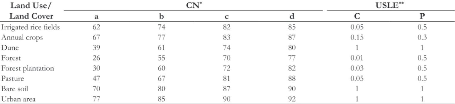
The peak low was estimated by the modiied rational formula. The surface runoff was calculated by the Soil Conservation Service curve number method (SCS-CN) (NEITSCH et al., 2011). The CN values deined for each land use/land cover class are presented in Table 1. The erosion caused by rainfall was calculated with the Modiied Universal Soil Loss Equation (MUSLE (WILLIAMS, 1975). The MUSLE equation enables simulating erosion from surface runoff. Equation 2 is as shown below:
0.56
11.8·( surf· peak· hru) · · · · ·
Sed= Q q area K C P LS CFRG (2)
where Sed is Sediment yield (t ha-1); Q
surf is Surface runoff volume
(mm ha-1); q
peak is Peak runoff rate (m
3 s-1); area
hru is Area of the
HRU (ha); K is USLE soil erodibility factor; C is USLE cover
and management factor; P is USLE support practice factor; LS is Topographic factor; CFRG is Coarse fragment factor.
The values selected for factor C (USLE cover and management factor) and factor P (USLE support practice factor) to estimate the erosion are shown in Table 1.
The low of solids through the channel network is based on deposition processes and degradation. The deposition within the channel to the exudate of the basin was determined from the deposition velocity of the sediment particles (MELO NETO et al., 2014). The sedimentation velocity was calculated from Stokes law and the sediment degradation in the canal was based on Bagnold’s concept of low power of Bagnold (1977).
Meteorological and hydro-sedimentological data
Meteorological monitoring was performed from ive DCPs installed in the study area (Figure 1). The following parameters were collected hourly, for a period of three years (from 2012 to 2015): temperature and relative air humidity, wind speed, precipitation, and solar radiation. To expand the series of climate data, a DCP installed from the river basin was used to extend the data set between the years 1981 and 2015.
TSS was monitored using multi-parametric probes coupled to hydro-sedimentological DCPs (Figure 1). The river level was measured in three sub-basins and the low was determined in the control section with the larger time frame (Figure 1). The key curve was established through the collection of hydrometric measurements, according to Equation 3:
( )1.284
1 0
0.0207 .
Q= N −N (3)
where Q is water low (m3 s-1); N
1 is water level in the control
section; N0 is water level in the monitoring section.
The amount of TSS was determined indirectly, from the correlation between nephelometric turbidity units (NTU) and TSS, collected between 2012 and 2015. The turbidity values were converted to TSS using Equation 4. Finally, the stream loads were determined by the product of the TSS content and the water low at the time.
( . . ) .
TSS= 0 8695 TURB 66 849+ (4)
where TSS is total suspended solids (mg L-1); TURB is turbidity
(NTU).
Calibration and validation of the hydrological model
The SWAT model was calibrated using the SWAT-CUP automated software. The Sequential Uncertainty Fitting algorithm (SUFI-2) was used for calibration and sensibility analysis.
This algorithm relies on user-deined simulations to map uncertainties on the parameters and try to capture the measured data with a prediction uncertainty rate of 95% (95PPU), using Latin hypercube sampling to calculate the levels of the accumulative distribution of an output variable. (ABBASPOUR et al., 2007).
Most of parameters selected in the calibration process are uncertainties in terms of the parameters themselves, inputs, or conceptual models that are dificult to measure in the ield. In addition, in Brazil there is little information available about these parameters. Thus, the range of values used in the calibration process was deined based on similar research (SANTHI et al., 2001; ANDRADE, 2011; ARNOLD et al., 2012b; BRIGHENTI; BONUMÁ; CHAFFE, 2016) and adjusted to represent natural processes from monitored hydro-sedimentological data.
The parameters, ranges, and values itted for the calibration process are shown in Table 2.
For the calibration, daily low and TSS data were collected between 1 Jan 2014 and 31 Dec 2014; validation was performed between 1 Jan 2015 and 31 Dec 2015. These periods were selected based on the series of monitoring data available for comparison with the data simulated by the model.
Evaluation criteria
To evaluate SWAT performance, the following precision statistics were used: Nash-Sutcliffe coeficient (NSE), Equation 5, and the residual mass coeficient (BIAS), described in Equation 6.
The perfect correlation between simulated and observed data is expressed as NSE = 1. Values of NSE < 0 demonstrate that using the mean of the observed values is better than the simulated results (BRIGHENTI; BONUMÁ; CHAFFE, 2016).
Table 1. Parameters describing the hydro-sedimentological processes of the river basin in each soil class.
Land Use/ Land Cover
CN* USLE**
a b c d C P
Irrigated rice ields 62 74 82 85 0.05 0.5
Annual crops 67 77 83 87 0.15 0.3
Dune 39 61 74 80 1 1
Forest 26 55 70 77 0.01 0.5
Forest plantation 30 60 72 82 0.03 0.5
Pasture 47 67 81 88 0.05 0.5
Bare soil 70 80 87 90 1 1
Urban area 77 85 90 92 1 1
Source: *Tucci (1993). **Arnold et al. (2012). (CN) curve number; (a) sandy soils, low clay content; (b) sandy soils, with a clay content > group A and < 15%; (c) soil
with a clay content between 20 and 30%; (d) clayey soils with > 30% clay content and low iniltration capacity; (C) USLE cover and management factor; (P) USLE
(
)
(
)
2 1
2 1
ni iobs isim
obs mean n
i i
V V
NSE
V V
=
=
−
=
−
∑ ∑
(5)
where NSE is Nash-Sutcliffe eficiency coeficient; n is total number of observations; ViOBS is observed value; V
i
SIM is simulated value;
Vmean is Mean of observed data in the period.
1 1
1
sim obs
n n
i i
i i
sim n
i i
V V
BIAS
V
= =
=
−
=
∑ ∑
∑
(6)
where BIAS is deviation; ViSIM is simulated value; V i
OBSis observed
value; n is total number of observations.
The trend between simulated and measured values is expressed by the BIAS coeficient. BIAS = 0% indicates a perfect relationship between the observed and the simulated data, positive values indicate underestimation, and negative values indicate overestimation of the simulated values.
To classify SWAT performance, the values defined by Santhi et al. (2001) were used: very good: NSE ≥ 0.65; good: 0.65 > NSE ≥ 0.54 and fair: 0.54 > NSE ≥ 0.50.
For BIAS, the scale proposed by Liew et al. (2007) was used: very good: |BIAS|≤ 10%; good: 10%<|BIAS|≤15%; fair: 15%<|BIAS| ≤ 25% and unsatisfactory: |BIAS|>25%.
Land use and occupation scenarios
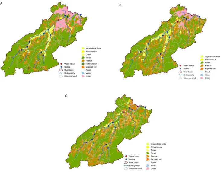
Three scenarios of land use and occupation were simulated. The scenarios were deined with differing input for the land use and occupation information. To create the layers, orthophotos corresponding to the years 2012, 1978, and 1957 were used, and renamed respectively to scenarios 1, 2, and 3 (Figure 2).
In the simulations, the parameters were adjusted in the model calibration (Table 2) using how baseline the scenario corresponding to the 2012. The same meteorological data, soil layer data, and digital elevation model were maintained for all three models.
The effect of changes in land use and occupation on the hydro-sedimentological dynamic was evaluated at the monitoring point at which water is taken for urban water supply - Water Intake (Figure 2) and in the outlets of the watershed. The three
scenarios were compared in order to identify patterns of change in the simulated variables.
The period from 2000 to 2005 was used to model simulation warm-up. This period is important for reducing systematic errors (ANDRADE, 2011), in that it guarantees that all components of water balance and sediment reached a state of equilibrium. Finally, the period between 2006 and 2015 was used for the analysis of results.
RESULTS AND DISCUSSION
Calibration and validation of the hydrological model
The results of low (m3 s-1) and TSS (t dia-1), as simulated
by SWAT, were compared with observed data (Figures 3 and 4). For the low, the NSE was 0.66 in the calibration and 0.89 in the daily validation (Figure 3). The results show a better results of the model in the validation (2015), possibly inluenced by the discrepancy between measured and simulated data in the calibration stage (2014) between March and mid-April (Figure 3). Possible causes of these results may be any of the following:
• Overestimation of precipitation measurements would have favored the overestimation of the simulated low rate; • Underestimation of water level measurements; this would
have contributed to the underestimation of the measured low;
• External factors – during this period, water was withdrawn for irrigation of the rice crop
BIAS indicates a small deviation between observed and simulated data, including underestimations of the low by 3% in the calibration and 14% in the validation.
According to the values of NSE and the scale developed by Santhi et al. (2001), the SWAT model provides highly accurate low estimations. In addition, the BIAS values indicate a performance level of “Good” in the calibration and “Very Good” in the validation (LIEW et al., 2007). Thus, the model was classiied as suitable for the simulation of land use scenarios in the CRB.
Figure 4 shows the comparison between measured and simulated TSS transported in the control section during execution
of the daily step. The sediment graph indicates strong adhesion between the measured and the simulated data. NSE was 0.80 in the calibration period (Figure 4), which is a strong result for NSE (according to SANTHI et al., 2001). The BIAS result of 0.24 indicates an underestimation of the simulated variable (LIEW et al., 2007) in calibration. For the validation period, NSE was 0.88 and BIAS was 0.12, indicating better performance in estimating the amount of TSS (Figure 4).
It is not always possible to identify the causes of variation between simulated and modeled data, but these results support the hypothesis regarding the overestimation of the precipitation and/or
Table 2. Parameters, ranges, and itted values in the process for
the SWAT calibration model.
Parameter Fitted
Value Range
1 Lat_Time 42 0 to 180
2 Esco 0.90 0 to 1
3 Gwqmin 1,000 0 to 5,000
4 Revapmn 1,000 0 to 1,000
5 Alpha_BF 0.60 0 to 1
6 Gw_delay 0.65 0 to 500
Lat_Time: lateral low travel time (day); Esco: soil evaporation compensation
factor; Gwqmin: threshold depth of water in the shallow aquifer required for return
low to occur (mm); Revapmn: threshold depth of water in the shallow aquifer
for “revap” or percolation to the deep aquifer to occur (mm); Alpha_Bf: base
low alpha factor (1/days); Gw_delay: groundwater delay (days).
Figure 3. Measured and simulated hydrograph for CRB on calibration data set (A) and validation (B), in the control watershed.
underestimation of the measured variable, as previously indicated for the low variable. Despite the variation between simulated and observed data, the statistics allow classifying the SWAT as very good, with a tendency to underestimate the simulated variable by 12%; this is satisfactory in studies using daily step calibration.
Land use land cover simulation scenarios
The main scientiic contribution of this study is to demonstrate the impact of land use/land cover changes on the water and sedimentological process in the Camboriú river basin. Table 3 shows the areas occupied with each class of activity for the simulated scenarios. The principal modiications were the urban class, pasture, and irrigated rice ields; there were signiicant increases in areas of urban use and rice ields, and some reduction of pasture between 1957 and 2012.
Flow simulation
The results of the land use/land cover scenarios were compared to each other to identify changes in hydrological behavior.
For this, the low permanence curves were initially generated for the three scenarios. This approach enables visualizing the behavior of the variable from the cumulative frequency of data over time. Figure 5 shows the average simulated daily low (m3 s-1) over
a 10-year period (2006–2015), classiied according to probability of occurrence. The water low associated with 100% probability is overcome in two scenarios, while discharge corresponding to a probability of 0% was not exceeded during the same period.
The results of water low from the simulated scenarios were classiied into ive ranges: base low, base low in dry conditions, intermediate
low, wet condition low and high low (Figure 5). This approach enables identifying the range that is most affected by the modiications in the land use/land cover scenarios. The base low and base low in
dry conditions ranges (exceedance probability > 60%) were most heavily affected, while the high low range (exceedance probability < 10%) was the second most heavily affected.
Comparing the results in the high low range, the highest values were recorded for the 2012 scenario, followed by the 1978 and 1957 scenarios. Selecting the low with an exceedance probability of less than 10% (Q10%), the 2012 scenario shows a low 16% higher than the Q10% recorded in the 1957 scenario.
In the base low and dry base low ranges, the 2012 scenario shows extreme conditions, followed by 1978 and 1957.
Several authors associate the alteration of landscape to changes in the hydrological regimen in watersheds, (ARABI et al., 2006; VANZELA; HERNANDEZ; FRANCO, 2010; BLAINSKI et al., 2011). Andréassian (2004) indicates that the increase of the forested area causes a decrease of the maximum peak low, and an increase in the base low discharge values. These changes can be attributed mainly to changes in evapotranspiration, roughness, and water iniltration rate in the soil.
In other similar studies, Bracmort et al. (2006) and Blainski et al. (2014) do not identify signiicant effects on the water regimen in the studied basins associated with modiications to land use/land cover.
This result suggests that the intrinsic diversity of the watershed characteristics could deine the degree of dependence between these two variables.
The results presented in this study make it possible to identify how changes in land use/land cover affect the hydrological regime of the CRB with more intensity at the extremes of the exceedance probability graph (Figure 5). For the scenarios of 2012 and 1978, an increase in the maximum peak lows of about 28.0% and 11.1%, respectively, were identiied. These changes are probably associated with the increase of irrigated rice ields, deforestation, and urban uses in these years. In addition, the emergence of early stages of forest plantation areas may have contributed to these results in the 2012 scenario. For the dry season, when compared to the 1957 scenario, the simulated low suffers a reduction of 11.1% and 33.3% corresponding to the same scenarios. In the intermediate stages, the difference between scenarios was not signiicant; the results fall within the range of uncertainty of the model, calculated at 0.56 m3 s-1 for this range.
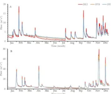
The hydrographs (Figure 6) for the water intake point (Figure 2) were generated in two years with different pluviometry volumes: 2006 – 1,409 mm year-1 (the lowest volume of annual
rainfall recorded) and 2008 – 2,474 mm year-1 (highest annual
accumulated rainfall). The results show that there was a change in the hydrological pattern caused by the change in land use/land cover, independent of the annual volume of precipitation.
In the 1957 scenario, the lowest low amplitudes were estimated. This means that in the dry period, the highest base lows were recorded and in the wet period, the lowest peak low
Table 3. Land use/land cover areas (ha) of the CRB by scenarios for 2012, 1978, and 1957.
LU/LC (ha) Year
2012 1978 1957
Water 98.7 38.4 37.7
Urban 1,571.3 649.4 22.0
Annual crops 69.6 131.7 415.8
Forest 12,095.6 11,627.2 12,479.8
Pasture 3,280.4 5,374.9 5,625.9
Bare soil 235.6 50.9 26.1
Rural roads 322.1 316.4 302.6
Irrigated rice ields 1,103.8 1,066.1 343.9
Forest plantation 477.9 0 0
Figure 5. Exceedance probability graph for daily low for a period
was recorded. This behavior suggests a tendency to smooth the luctuations of the hydrograph curve.
In the 2012 scenario, for the two cases (Figures 6A and 6B), the lowest base low rates were recorded in dry conditions and the highest peak lows in wet conditions, thus corroborating the results obtained in other studies that associate the increase of high lows to the replacement of natural landscapes by agricultural or urban uses (ANDRÉASSIAN, 2004; ARABI, et al., 2006; VANZELA; HERNANDEZ; FRANCO, 2010; BLAINSKI et al., 2011).
Soil erosion simulation
Estimation of erosion rates and identiication of areas with the highest occurrence are important components of river basin management. Figure 7 shows the mean distribution of simulated erosion in the land use/land cover scenarios for the speciied sub-basins.
In the 1957 scenario, the lowest rates of soil loss were identiied. The scenario has a low amount of urban area and the smallest area of irrigated rice ields among the three simulated
Figure 6. Simulated hydrographs in the three scenarios (m3 s-1) for
the water intake watershed, in two years with distinct pluviometry characteristics; A-2006 (low rainfall year) and B-2008 (high rainfall year).
scenarios (Table 3). The maximum soil loss was 14.6 t ha-1 year-1.
Excluding the sub-watershed 5, soil loss was lower than 8.0 t ha-1 year-1
(Figure 7); in about 48% of the river basin area, the erosion rate was below 5.0 t ha-1 year-1.
In sub-watershed 5, about 36% of the area is occupied by pasture and 8.2% by irrigated rice ields. According Brooks et al. (1991), pastures associated with steep terrain and/or erosion-susceptible soils may have a high rate of soil loss, which probably explains the data recorded in this area. The authors also explain that sediment production increases when the riparian zone is also used for pasture, increasing erosion of the river bank and the eventual deposition of sediments in the river bed.
Another important factor related to soil loss and forest land cover, according to Wischmeier and Smith (1978), is the natural erosion control produced by the forest cover; they found that the interception and vegetal cover protect the soil surface from the direct impact of raindrops. Furthermore, forest cover promotes improvement in soil structure and iniltration rates, and an increase in water retention capacity; in addition, the soil roughness characteristics increase surface friction, which generates a decrease in surface runoff velocity (BERTONI; LOMBARDI NETO, 2010).
In the 1978 scenario, soil loss was numerically higher than in the 1957 scenario (Figure 7), mainly in sub-basins in which the change in soil use was more intense.
In sub-watershed 5, soil erosion was estimated to be 41.0 t ha-1 year-1. The high rate can be attributed to land use
alterations and their implications for related processes, such as water iniltration capacity, runoff, conservation practices, and crop management.
For the same area, in 1957, the irrigated rice ields occupied about 8.2% of the total area, while forested areas extended to 52.0% of the total sub-basin. In the 1978 scenario, the rice crops increased against a decrease of the forested areas, causing the percentages to change to 36.5% and 29.4%, for rice and forests respectively. Similar behavior was observed in sub-basins 9, 8, and 3 (Figure 2).
In the 2012 scenario, soil loss was higher than in other scenarios (Figure 7). Thus, as previously reported, the substitution of forested areas for agricultural uses was the main factor associated with an increase of soil loss. In this particular scenario, the irrigated rice ields increased for the middle river basin, the site with the highest rates of soil loss (Figure 7). Compared to the 1978 scenario, in sub-watershed 5 and 12, the reduction of soil loss is mainly due to the increase of forested areas and the decrease of pasture areas. In addition, in sub-watersheds 1, 2, and 4, the increased rate of erosion was mainly due to the reduction of forested areas and the increase of irrigated rice ields.
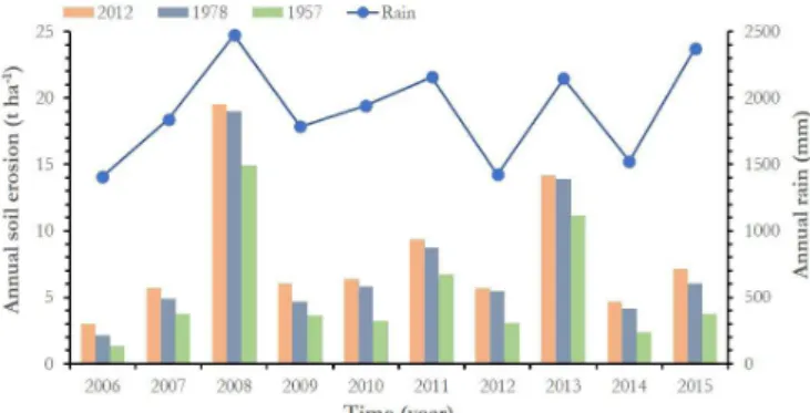
Figure 8 shows the average soil erosion in the river basin estimated from each simulated scenario, from 2006 to 2015. The results compare variations in soil erosion for the proposed scenarios and the temporal variations in the simulated years.
As previously reported, variations in land use/land cover that were identiied among the studied scenarios could be the main causes of the variations in soil erosion rates in the CRB.
The temporal variations observed in the erosion estimates can be attributed to strong variations in the recorded volume of precipitation. This parameter is directly correlated to the surface
runoff rate and contributes to the increase of the low water and the related volume of transported solids.
The variations in precipitation recorded between 2006 and 2008 relect a signiicant change in the erosion rate, independent of the simulated scenarios. For the 1957 scenario, characterized by the lower inluence of human activity, average soil erosion was 1.40 t ha-1 year-1 and annual precipitation was 1,409 mm. In the
same scenario in 2008, annual rainfall reached 2,474 mm and soil loss was about 14.8 t ha-1 year-1.
The results in Figure 8 demonstrate the strong inluence of rainfall on the soil erosion process, perhaps inluenced by the increase in runoff rate in years characterized by high rainfall rates (Figure 9).
Throughout the studied period, the highest surface runoff rate was found in the 2012 scenario, followed by the 1978 and 1957 scenarios, respectively. Changes in vegetal cover (Table 1) resulted in changes in the roughness coeficient and the water iniltration rate; consequently, scenarios with the highest surface runoff rates are those having a higher number of areas with exposed soil, irrigated rice ields, and urban areas.
A considerable portion of the CRB lies within the accepted limits for estimated erosion rates (BLAINSKI et al., 2011), considering the type of soils and the topography factors in the study region. According to the authors, in the Ribeirão Gustavo (SC) river basin, with soil and climatic characteristics similar to the study area, the average tolerance to soil erosion was estimated at 7.83 t ha year-1. Therefore, for the 1957 and 1978 scenarios, and
Figure 8. Soil erosion simulations for 2012, 1978, and 1957 for the CRB.
in the sub-watershed with the largest forested area, soil loss falls within naturally tolerable values.
However, the results indicate that the soil and climatic characteristics could increase soil degradation, especially in years with high volumes of rainfall. In addition, Figure 7 shows the impact of replacing natural landscapes with agricultural activities, in this case rice crops and pasture land. The higher rate of soil loss is linked to watersheds where land use classes related to human activity were predominant, or in sub-watersheds where soil loss was notoriously greater than in the areas occupied by forests.
The principal factor related to the increased rate of soil loss in the crop-related land use classes is excessive tilling methods, which can cause soil compaction, loss of iniltration capacity, and high susceptibility of these soils to erosion. In pasture areas, this increase in erosion may be associated with the reduction of the natural vegetation cover, soil compaction by animal trampling, and lack of conservation practices. This combination of factors, in association with areas of high slope, signiicantly increases the velocity of surface runoff, and consequently, soil loss.
Finally, the change in land use and occupation results in a signiicant change in the hydric and sediment regimen of the CRB. In the literature, numerous papers describe the role of vegetal cover in controlling soil loss and increasing water availability (PANACHUKI et al., 2011; CARDOSO et al., 2012; DIAS, 2012; GALHARTE et al., 2014; PEREIRA et al., 2014). In this work, however, through hydrological modeling, it was possible simulate the landscape changes recorded over 55 years of occupation and their impacts on the hydrosedimentological dynamic, generating strategic information for the management of the hydrographic basin and for the prioritization of interventions seeking environmental preservation and the sustainability of agricultural activities.
CONCLUSION
In this study, adjustments to the SWAT calibration parameters provided satisfactory coniguration for modeling the discharge and sediment regimen of the CRB. Thus, it was possible to quantify the changes in the variables of low for three land use/land cover scenarios, TSS, and soil loss in this river basin.
The main simulated low changes in the scenarios for 1957, 1978, and 2012 occurred at the extremes of the probability of exceedance. In the intermediate range, the differences remained close to the model’s uncertainty range.
For soil loss, sub-basins with predominantly agricultural uses showed the highest values. However, in the period studied, the CRB did not report severe problems of soil loss. The results also indicate that soil and climatic characteristics may favor soil degradation, especially in years with a high volume of precipitation.
ACKNOWLEDGEMENTS
The authors are grateful to CNPq (processes 478153 / 2012-0, 403739 / 2013-6 and 303472 / 2014-6) for promoting research and conferring a research productivity grant.
REFERENCES
ABBASPOUR, K. C.; YANG, J.; MAXIMOV, I.; SIBER, R.; BOGNER, K.; MIELEITNER, J.; ZOBRIST, J.; SRINIVASAN, R. Modelling of hydrology and water quality in the pre-alpine/alpine Thur watershed using SWAT. Journal of Hydrology, v. 333, n. 2-4, p. 413-430, 2007. http://dx.doi.org/10.1016/j.jhydrol.2006.09.014.
ALLEN, R. G.; JENSEN, M. E.; WRIGHT, J. L.; BURMAN, R. D. Operational estimates of reference evapotranspiration. Agronomy Journal, v. 81, n. 4, p. 650-662, 1989. http://dx.doi.org/10.2134/ agronj1989.00021962008100040019x.
ANDRADE, M. A. Simulação hidrológica numa bacia hidrográica
representativa dos latossolos na região Alto Rio Grande. 2011. 102 f. Dissertação (Mestrado) - Universidade Federal de Lavras, Lavras, 2011.
ANDRÉASSIAN, V. Water and forests: from historical controversy to scientific debate. Journal of Hydrology, v. 291, n. 1-2, p. 1-27, 2004. http://dx.doi.org/10.1016/j.jhydrol.2003.12.015.
ARABI, M.; GOVINDARAJU, R. S.; HANTUSH, M. M.; ENGEL, B. A. Role of watershed subdivision on modeling the effectiveness of best management practices with SWAT. Journal of the American
Water Resources Association, v. 42, n. 2, p. 513-528, 2006. http:// dx.doi.org/10.1111/j.1752-1688.2006.tb03854.x.
ARNOLD, J. G.; KINIRY, J. R.; SRINIVASAN, R.; WILLIAMS, J. R.; HANEY, E. B.; NEITSCH, S. Soil and Water Assessment Tool
input/output ile Documentation: Version 2012. Texas: Texas Water Resources Institute, 2012a. 654 p.
ARNOLD, J. G.; MORIASI, D. N.; GASSMAN, P. W.; ABBASPOUR, K. C.; WHITE, M. J.; SRINIVASAN, R.; SANTHI, C.; HARMEL, R. D.; VAN GRIENSVEN, A.; VAN LIEW, M. W.; KANNAN, N.; JHA, M. K. SWAT: model use calibration and validation.
Transactions of the ASABE, v. 55, n. 4, p. 1494-1508, 2012b. http:// dx.doi.org/10.13031/2013.42256.
BAGNOLD, R. A. Bed load transport by natural rivers. Water
Resources Research, v. 13, n. 1, p. 303-312, 1977. http://dx.doi. org/10.1029/WR013i002p00303.
BAKER, T. J.; MILLER, S. N. Using the Soil and Water Assessment Tool (SWAT) to assess land use impact on water resources in an east African watershed. Journal of Hydrology, v. 486, n. 1, p. 100-111, 2013. http://dx.doi.org/10.1016/j.jhydrol.2013.01.041.
BALTOKOSKI, V.; TAVARES, M. H. F.; MACHADO, R. E.; OLIVEIRA, M. P. Calibração de modelo para a simulação de vazão e de fósforo total nas sub-bacias dos rios Conrado e Pinheiro – Pato Branco (PR). Revista Brasileira de Ciencia do Solo, v. 34, n. 1, p. 253-261, 2010. http://dx.doi.org/10.1590/S0100-06832010000100026.
using a physical process model. Agriculture, Ecosystems & Environment, v. 113, n. 1-4, p. 62-72, 2006. http://dx.doi.org/10.1016/j. agee.2005.08.032.
BERTONI, J.; LOMBARDI NETO, F. Conservação do solo. São Paulo: Ícone, 2010. 355 p.
BEVEN, K. Rainfall-Runoff Modelling: the primer. West Sussex: John Wiley & Sons, 2001. 360 p.
BLAINSKI, É.; DORTZBACH, D.; PEREIRA, A. P. E.; FARIAS, M. G. Uso de modelo hidrossedimentológico para a simulação de cenários de uso da terra na microbacia Ribeirão Gustavo, Santa Catarina. Revista de Gestão de Água da América Latina, v. 11, n. 1, p. 21-32, 2014.
BLAINSKI, E.; SILVEIRA, F. A.; CONCEIÇÃO, G.; GARBOSSA, L. H. P.; VIANNA, L. F. Simulação de cenários de uso do solo na bacia hidrográfica do rio Araranguá utilizando a técnica da modelagem hidrológica. Agropecuária Catarinense, v. 24, n. 1, p. 65-70, 2011.
BONUMÁ, N. B.; REICHERT, J. M.; RODRIGUES, M. F.; MONTEIRO, J. A. F.; ARNOLD, J. G.; SRINIVASAN, R. Modeling surface hydrology, soil erosion, nutrient transport and future scenarios with the ecohydrological SWAT model in Brazilian watersheds and river basins. Tópicos em Ciência do Solo, v. 9, p. 241-290, 2015.
BOURAOUI, F.; VACHAUD, G.; HAVERKAMP, R.; NORMAND, B. A distributed physical approach for surface-subsurface water transport modeling in agricultural watersheds. Journal of Hydrology, v. 203, n. 1-4, p. 79-92, 1997. http://dx.doi.org/10.1016/S0022-1694(97)00085-1.
BRACMORT, K. S.; ARABI, M.; FRANKENBERGER, J. R.; ENGEL, B. A.; ARNOLD, J. G. Modeling long-term water quality impact of structural BMPs. Transactions of the ASABE, v. 49, n. 2, p. 367-374, 2006. http://dx.doi.org/10.13031/2013.20411.
BRESSIANI, D. A.; GASSMAN, P. W.; FERNANDES, J. G.; GARBOSSA, L.; SRINIVASAN, R.; BONUMA, N. B.; MENDIONDO, E. M. A review of Soil and Water Assessment Tool (SWAT) applications in Brazil: challenges and prospects.
International Journal of Agricultural and Biological Engineering, v. 8, n. 3, p. 1-27, 2015.
BRIGHENTI, T. M.; BONUMÁ, N. B.; CHAFFE, P. L. B. Calibração hierárquica do modelo Swat em uma bacia hidrográfica Catarinense. Revista Brasileira de Recursos Hídricos, v. 21, n. 1, p. 53-64, 2016. http://dx.doi.org/10.21168/rbrh.v21n1.p53-64.
BROOKS, K. N.; FFOLLIOTT, P. F.; GREGERSEN, H. M.; THAMES, J. L. Hydrology and the management of watersheds. Ames: Iowa State University Press, 1991. 392 p.
CAN, T.; XIAOLING, C.; JIAMZHONG, L.; GASSMAN, P. W.; SAUVAGE, S.; PÉREZ, J. M. S. Assessing impacts of different
land use scenarios on water budget of Fuhe River, China using SWAT model. International Journal of Agricultural & Biological Engineering, v. 8, n. 3, 2015.
CARDOSO, D. P.; SILVA, M. L. N.; CARVALHO, G. J.; FREITAS, D. A. F.; AVANZI, J. C. Plantas de cobertura no controle das perdas de solo, água e nutrientes por erosão hídrica. Revista Brasileira de
Engenharia Agrícola e Ambiental, v. 16, n. 6, p. 632-638, 2012. http:// dx.doi.org/10.1590/S1415-43662012000600007.
DIAS, A. C. Plantas de cobertura do solo na atenuação da erosão hídrica no
sul do Estado de Minas Gerais. 2012. 111 f. Dissertação (Mestrado)-Universidade Federal de Lavras, Lavras, 2012.
EMBRAPA – EMPRESA BRASILEIRA DE PESQUISA AGROPECUÁRIA. Centro Nacional de Pesquisa de Solos. Sistema
brasileiro de classiicação de solos. 3. ed. Brasília: Embrapa, 2013. 353 p.
GALHARTE, C. A.; VILLELA, J. M.; CRESTANA, S. Estimativa da produção de sedimentos em função da mudança de uso e cobertura do solo. Revista Brasileira de Engenharia Agrícola e Ambiental, v. 18, n. 1, p. 194-201, 2014.
GHAFFARI, G.; KEESSTRA, S.; GHODOUSI, J.; AHMADI, H.. SWAT-simulated hydrological impact of land-use change in the Zanjanrood Basin, Northwest Iran. Hydrological Processes, v. 24, n. 7, p. 892-903, 2010. http://dx.doi.org/10.1002/hyp.7530.
GREEN, C. H.; VANGRIENSVEN, A. Autocalibration in hydrologic modeling: using SWAT 2005 in small-scale watersheds.
Environmental Modelling & Software, v. 23, n. 1, p. 422-434, 2008. http://dx.doi.org/10.1016/j.envsoft.2007.06.002.
GRIGG, N. S. Water resources management: principles, regulations, and
cases. Nova Iorque: McGraw-Hill Book, 1996. 540 p.
LELIS, T. A.; CALIJURI, M. L.; SANTIAGO, A. F.; LIMA, D. C.; ROCHA, E. O. Análise de sensibilidade e calibração do modelo SWAT aplicado em bacia hidrográfica da região sudeste do Brasil. Revista Brasileira de Ciencia do Solo, v. 36, n. 2, p. 623-634, 2012. http://dx.doi.org/10.1590/S0100-06832012000200031.
LIEW, M. W.; VEITH, T. L.; BOSCH, D. D.; ARNOLD, J. G. Suitability of SWAT for the Conservation effects assessment project: A comparison on USDA-ARS watersheds. Journal of
Hydrology Resources, v. 12, n. 2, p. 173-189, 2007.
MACHADO, R. E.; VETORAZZI, C. A.; XAVIER, A. C. Simulação de cenários alternativos de uso da terra em uma microbacia utilizando técnicas de modelagem e geoprocessamento. Revista
Brasileira de Ciencia do Solo, v. 27, n. 4, p. 727-733, 2003. http:// dx.doi.org/10.1590/S0100-06832003000400017.
MAIDMENT, D. R. GIS and hydrologic modeling. In: GOODCHILD, M. F.; PARKS, B. O.; STEYAERT, L. T. (Ed.). Environmental
MELO NETO, J. O.; SILVA, A. M.; MELLO, C. R.; MELLO JÚNIOR, A. V. Simulação hidrológica escalar com o modelo SWAT. Revista Brasileira de Recursos Hídricos, v. 19, n. 1, p. 177-188, 2014. http://dx.doi.org/10.21168/rbrh.v19n1.p177-188.
NEITSCH, S. L.; ARNOLD, J. G.; KINIRY, J. R.; WILLIAMS, J. R. Soil and water assessment tool: theoretical documentation. Version
2009. Texas: Grassland, Soil and Water Research Laboratory, Agricultural Research Service, Blackland Research Center, Texas AgriLife Research, 2011. 618 p.
PANACHUKI, E.; BERTOL, I.; ALVES SOBRINHO, T.; OLIVEIRA, P. T. S.; RODRIGUES, D. B. B. Perdas de solo e de água e infiltração de água em Latossolo Vermelho sob sistemas de manejo. Revista Brasileira de Ciência do Solo, v. 35, n. 5, p. 1777-1785, 2011. http://dx.doi.org/10.1590/S0100-06832011000500032.
PANDOLFO, C.; BRAGA, H. J.; SILVA JUNIOR, V. P.; MASSIGNAM, A. M.; PEREIRA, E. S.; THOMÉ, V. M. R.; VALCI, F. V. Atlas climatológico digital do Estado de Santa Catarina. Florianópolis: Epagri, 2002. CD-ROM.
PEREIRA, D. R.; ALMEIDA, A. Q.; MARTINEZ, M. A.; ROSA, D. R. Q. Impacts of deforestation on water balance components of a watershed on the Brazilian East Coast. Revista Brasileira de
Ciência do Solo, v. 38, n. 4, p. 1350-1358, 2014. http://dx.doi. org/10.1590/S0100-06832014000400030.
PIKOUNIS, M.; VARANOU, E.; BALTAS, E.; DASSAKLIS, A.; MIMIKOU, M. Application of SWAT model in the Pinios River Basin under different land-use scenarios. Global Nest: the International Journal, v. 5, n. 2, p. 71-79, 2003.
REUNGSANG, P.; KANWAR, R. S.; JHA, M.; GASSMAN, P. W.; AHMAD, K.; SALEH, A. Calibration and validation of SWAT for the upper Maquoketa River Watershed. International Journal of
Agriculture and Engineering, v. 16, n. 1, p. 35-48, 2009.
SANTHI, C.; ARNOLD, J. G.; WILLIAMS, J. R.; DUGAS, W. A.; SRINIVASAN, R.; HAUCK, L. M. Validation of the SWAT model on a large river basin with point and nonpoint sources. Journal of
the American Water Resources Association, v. 37, n. 5, p. 1169-1188, 2001. http://dx.doi.org/10.1111/j.1752-1688.2001.tb03630.x.
SILVA, V. A.; MOREAU, M. S.; MOREAU, A. M. S. S.; REGO, N. A. C. Uso da terra e perda de solo na Bacia Hidrográfica do Rio
Colônia, Bahia. Revista Brasileira de Engenharia Agrícola e Ambiental, v. 15, n. 3, p. 310-315, 2011. http://dx.doi.org/10.1590/S1415-43662011000300013.
STEYAERT, L. T. A perspective on the state of environmental simulation modeling. In: GOODCHILD, M. F.; PARKS, B. O.; STEYAERT, L. T. (Ed.). Environmental modeling with GIS. New York: Oxford University Press, 1993. Cap. 3, p. 16-30.
TUCCI, C. E. M. Hidrologia: ciência e aplicação. Porto Alegre: UFRGS-ABRH, 1993. 952 p.
TUCCI, C. E. M. Modelos hidrológicos. Porto Alegre: UFRGS-ABRH, 2005. 678 p.
VANZELA, L. S.; HERNANDEZ, F. B. T.; FRANCO, A. M. Influência do uso e ocupação do solo nos recursos hídricos do Córrego Três Barras, Marinópolis. Revista Brasileira de Engenharia
Agrícola e Ambiental, v. 14, n. 1, p. 55-64, 2010. http://dx.doi. org/10.1590/S1415-43662010000100008.
WILLIAMS, J. R. Sediment routing for agricultural watersheds.
Water Resources Bulletin, v. 11, n. 5, p. 965-974, 1975. http://dx.doi. org/10.1111/j.1752-1688.1975.tb01817.x.
WISCHMEIER, W. H.; SMITH, D. D. P. Redicting rainfall erosion losses: a guide to conservation planning. Washington: Department of Agriculture, 1978. 58 p. (Agriculture Handbook, 537).
Authors contributions
Éverton Blainski: Responsible for paper conception, research, data analysis, literature review, discussion and paper writing.
Eileen Andrea Acosta Porras: Collaborations in SWAT calibration, data analysis, writing and translate.
Luis Hamilton Pospissil Garbossa: Responsible for multiparameter probe implantation, writing and revision.