A Protein Sequence Analysis Hardware Accelerator Based on Divergences

Volume 2012, Article ID 201378,19pages doi:10.1155/2012/201378

Research Article

A Protein Sequence Analysis Hardware Accelerator

Based on Divergences

Juan Fernando Eusse,

_{Nahri Moreano,}

_{Alba Cristina Magalhaes Alves de Melo,}

and Ricardo Pezzuol Jacobi

1_{Electrical Engineering Department, University of Brasilia, Brasilia, DF 70910-900, Brazil}

2_{School of Computing, Federal University of Mato Grosso do Sul, Campo Grande, MS 79070-900, Brazil} 3_{Computer Science Department, University of Brasilia, Brasilia, DF 70910-900, Brazil}

4_{UnB Gama School, University of Brasilia, Gama, DF 72405-610, Brazil}

Correspondence should be addressed to Ricardo Pezzuol Jacobi,[email protected]

Received 27 September 2011; Accepted 26 December 2011

Academic Editor: Khaled Benkrid

Copyright © 2012 Juan Fernando Eusse et al. This is an open access article distributed under the Creative Commons Attribution License, which permits unrestricted use, distribution, and reproduction in any medium, provided the original work is properly cited.

The Viterbi algorithm is one of the most used dynamic programming algorithms for protein comparison and identification, based on hidden markov Models (HMMs). Most of the works in the literature focus on the implementation of hardware accelerators that act as a prefilter stage in the comparison process. This stage discards poorly aligned sequences with a low similarity score and forwards sequences with good similarity scores to software, where they are reprocessed to generate the sequence alignment. In order to reduce the software reprocessing time, this work proposes a hardware accelerator for the Viterbi algorithm which includes the concept of divergence, in which the region of interest of the dynamic programming matrices is delimited. We obtained gains of up to 182x when compared to unaccelerated software. The performance measurement methodology adopted in this work takes into account not only the acceleration achieved by the hardware but also the reprocessing software stage required to generate the alignment.

1. Introduction

Protein sequence comparison and analysis is a repetitive task in the field of molecular biology, as is needed by biologists to predict or determine the function, structure, and evolutional characteristics of newly discovered protein sequences. During the last decade, technological advances had made possible the identification of a vast number of new proteins that have been introduced to the existing protein databases [1, 2]. With the exponential growth of these databases, the execution times of the protein comparison algorithms also grew exponentially [3], and the necessity to accelerate the existing software rose in order to speed up research.

The HMMER 2.3.2 program suite [4] is one of the most used programs for sequence comparison. HMMER takes multiple sequence alignments of similar protein sequences grouped into protein families and builds hidden Markov models (HMMs) [5] of them. This is done to estimate

statistically the evolutionary relations that exist between different members of the protein family, and to ease the identification of new family members with a similar struc-ture or function. HMMER then takes unclassified input sequences and compares them against the generated HMMs of protein families (profile HMM) via the Viterbi algorithm (see Section 2), to generate both a similarity score and an alignment for the input (query) sequences.

of the Viterbi algorithm, while achieving a better cost/benefit relation than the cluster approach.

Studies have also shown that most of the processing time of the HMMER software is spent into processing poor scoring (nonsignificant) sequences [11], and most authors have found useful to apply a first-phase filter in order to discard poor scoring sequences prior to full processing. Some works apply heuristics [12], but the mainstream focuses on the use of FPGA-based accelerators [3,11,13–16] as a first-phase filter. The filter retrieves the sequence’s similarity score and, if it is acceptable, instructs the software to reprocess the sequence in order to generate the corresponding alignment.

Our work proposes further acceleration of the algorithm by using the concept of divergence in which full reprocessing of the sequence after the FPGA accelerator is not needed, since the alignment only appears in specific parts of both the profile HMM model and the sequence. The proposed accel-erator outputs the similarity score and the limits of the area of the dynamic programming (DP) matrices that contains the optimal alignment. The software then calculates only that small area of the DP matrices for the Viterbi algorithm and returns the same alignment as the unaccelerated software.

The main contributions of this work are threefold. First, we propose the Plan7-Viterbi divergence algorithm, which calculates the area in the Plan7-Viterbi dynamic program-ming matrices that contains the sequence-profile alignment. Second, we propose an architecture that implements this algorithm in hardware. Our architecture not only is able to generate the score for a query sequence when compared to a given profile HMM but also generates the divergence algorithm coefficients in hardware, which helps to speed up the subsequent alignment generation process by software. To the best of our knowledge, there is no software adaptation of the divergence algorithm to the Viterbi-Plan7 algorithm nor a hardware implementation of that adaptation. Finally, we propose a new measurement strategy that takes into account not only the architecture’s throughput but also reprocessing times. This strategy helps us to give a more realistic measure of the achieved gains when including a hardware accelerator into the HMMER programs.

This work is organized as follows. InSection 2we clarify some of the concepts of protein sequences, protein families, and profile HMMs. InSection 3we present the related work in FPGA-based HMMER accelerators.Section 4introduces the concept of divergences and their use in the acceleration of the Viterbi algorithm. Section 5 shows the proposed hardware architecture. Section 6 presents the metrics used to analyze the performance of the system. In Section 7 we show implementation and performance results, and we compare them with the existing works. Finally, inSection 8 we summarize the results and suggest future works.

2. Protein Sequence Comparison

2.1. Protein Sequences, Protein Families, and Profile HMMs. Proteins are basic elements that are present in every living organism. They may have several important functions such as catalyzing chemical reactions and signaling if

a gene must be expressed, among others. Essentially, a protein is a chain of amino acids. In the nature, there are 20 different amino acids, represented by the alphabet Σ= {A,C,D,E,F,G,H,I,K,L,M,N,P,Q,R,S,T,V,W,Y}

[17].

A protein family is defined to be a set of proteins that have similar function, have similar 2D/3D structure, or have a common evolutionary history [17]. Therefore, a newly sequenced protein is often compared to several known protein families, in search of similarities. This comparison usually aligns the protein sequence to the representation of a protein family. This representation can be a profile, a consensus sequence, or a signature [18]. In this paper, we will only deal with profile representations, which are based on multiple sequence alignments.

Given a multiple-sequence alignment, a profile specifies, for each column, the frequency that each amino acid appears in the column. If a sequence-profile comparison results in high similarity, the protein sequence is usually identified to be a member of the family. This identification is a very important step towards determining the function and/or structure of a protein sequence.

One of the most accepted probabilistic models to do sequence-profile comparisons is based on hidden Markov models (HMMs). It is called profile HMM because it groups the evolutionary statistics for all the family members, therefore “profiling” it. A profile HMM models the common similarities among all the sequences in a protein family as discrete states; each one corresponding to an evolution-ary possibility such as amino acid insertions, deletions, or matches between them. The traditional profile HMM architecture proposed by Durbin et al. [5] consisted of insert (I), delete (D), and match (M) states.

The HMMER suite [4], is a widely used software imple-mentation of profile HMMs for biological sequence analysis, composed of several programs. In particular, the program hmmsearchsearches a sequence database for matches to an HMM, while the program hmmpfam searches an HMM database for matches to a query sequence.

HMMER uses a modified HMM architecture that in addition to the traditional M, I, and D states includes flanking states that enable the algorithm to produce global or local alignments, with respect to the model or to the sequence, and also multiple-hit alignments [4,5]. The Plan7 architecture used by HMMER is shown inFigure 1. Usually, there is one match state for each consensus column in the multiple alignment. EachMstate aligns to (emits) a single residue, with a probability score that is determined by the frequency in which the residues have been observed in the corresponding column of the multiple alignment. Therefore, eachM state has 20 probabilities for scoring the 20 amino acids.

B S T E N C J Main states Flanking states M1 M2 M3 M4

I1 I2 I3

D2 D3

Figure_{1: Plan7 architecture used by HMMER [3].}

B S T E N C J 0 0 0

I1 I2 I3

M1 M2 M3 M4

D2 D3

−1

−1 −1

−1 −1 −1

−1

−2 −2 −2

−2

−2

−3 −3−3

−3 −3

−3−3 −3−3

−3

−3

−3

−3

−4 −4

−∞

−∞ −∞

Figure_{2: A profile HMM with 4 nodes and the transition scores.}

probabilities, there are transition probabilities associated to each transition from one state to another.

2.2. Viterbi Algorithm. Given a HMM modeling a protein family and a query sequence, HMMER computes the proba-bility that the sequence belongs to the family, as a similarity score, and generates the resulting alignment if the score is sufficiently good. To do so, it implements a well-known DP algorithm called the Viterbi algorithm [19]. This algorithm calculates a set of score matrices (corresponding to statesM, I, andD) and vectors (corresponding to states N, B, E, C, andJ) by means of a set of recurrence equations. As a result, it finds the best (most probable) alignment and its score for the query sequence with the given model.

Equations (1) show the Viterbi algorithm recurrence relations for aligning a sequence of length n to a profile HMM withknodes. In these equations,M(i,j) is the score of the best path aligning the subsequence s1. . . si to the

submodel up to stateMj andI(i,j) andD(i,j) are defined

similarly. The emission probability of the amino acid si

at state1 is denoted by em(state1,si), while tr(state1,state2) represents the transition cost from state1 to state2. The similarity score of the best alignment is given byC(n) + tr(C, T).

Plan7-Viterbi algorithm recurrence equations, for a profile HMM with knodes and sequence sof lengthnare as follows;

M(i, 0)=I(i, 0)=D(i, 0)= −∞ ∀1≤i≤n,

M 0,j =I 0,j =D 0,j

= −∞ ∀0≤j≤k,

M

i,j

=emMj,si + max ⎧ ⎪ ⎪ ⎪ ⎪ ⎪ ⎪ ⎪ ⎪ ⎨ ⎪ ⎪ ⎪ ⎪ ⎪ ⎪ ⎪ ⎪ ⎩ M

i−1,j−1

+ trMj−1,Mj

I

i−1,j−1

+ trIj−1,Mj

D

i−1,j−1

+ trDj−1,Mj

B(i−1) + trB,Mj

∀1≤i≤n,

I

i,j

=emIj,si + max ⎧ ⎪ ⎨ ⎪ ⎩ M

i−1,j

+ trMj,Ij

I

i−1,j

+ trIj,Ij

∀1≤j≤k,

D

i,j =max ⎧ ⎪ ⎨ ⎪ ⎩ M

i,j−1

+ trMj−1,Dj

D

i,j−1

+ trDj−1,Dj

,

N(0)=0,

N(i)=N(i−1) + tr(N,N), ∀1≤i≤n,

B(0)=tr(N,B),

B(i)=max

⎧ ⎨

⎩

N(i) + tr(N,B)

J(i) + tr(J,B)

∀1≤i≤n,

E(i)=max 1≤j≤k

M

i,j

+trMj,E

∀1≤j≤k,

J(0)= −∞,

J(i)=max

⎧ ⎨

⎩

J(i−1) + tr(J,J)

E(i) + tr(E,J)

∀1≤i≤n,

C(0)= −∞,

C(i)=max

⎧ ⎨

⎩

C(i−1) + tr(C,C)

E(i) + tr(E,C)

∀1≤i≤n.

similarity score=C(n) + tr(C,T).

(1)

Figure 2illustrates a profile HMM with 4 nodes repre-senting a multiple-sequence alignment. The transition scores are shown in the figure, labeling the state transitions. The emission scores for theMandIstates are shown inTable 1.

Table_{1: Emission scores of amino acids for match and insert states of profile HMM ofFigure 2.}

State A C D E F, I, L, M, V, W G, K, P, S H, Q, R, T Y

M1 7 −1 −1 1 −1 2 1 −1

M2 −1 9 −1 1 −1 2 1 −1

M3 −1 −1 8 2 −1 2 1 −1

M4 −1 −1 3 9 −1 2 1 −1

I1 −1 −1 0 1 −1 0 1 2

I2 −1 −1 0 1 −1 0 1 2

I3 −1 −1 0 1 −1 0 1 2

Table_{2: Score matrices and vectors of the Viterbi algorithm for the comparison of the sequence ACYDE against the profile HMM ofFigure 2.}

N B M I D E J C

0 1 2 3 4 0 1 2 3 4 0 1 2 3 4

— 0 0 −∞ −∞ −∞ −∞ −∞ −∞ −∞ −∞ −∞ −∞ −∞ −∞ −∞ −∞ −∞ −∞ −∞ −∞

A −1 −1 −∞ −5 −4 −4 −4 −∞ −∞ −∞ −∞ −∞ −∞ −∞ 1 −1 −3 2 −∞ 2

C −2 −2 −∞ −4 13 −1 −3 −∞ 1 −8 −8 −8 −∞ −∞ −8 9 7 10 −∞ 10

Y −3 −3 −∞ −5 −3 11 7 −∞ 1 12 2 −4 −∞ −∞ −9 −7 7 8 −∞ 9

D −4 −4 −∞ −6 −3 17 13 −∞ −1 10 8 6 −∞ −∞ −10 −7 13 14 −∞ 14

E −5 −5 −∞ −5 −3 9 25 −∞ −2 9 15 24 −∞ −∞ −9 −7 5 25 −∞ 25

the path (S,-) → (N,-) → (B,-) → (M1,A) → (M2,C) →

(I2,Y)→ (M3,D)→ (M4,E)→ (E,-) →(C,-)→ (T,-).

3. Related Work

The function that implements the Viterbi algorithm in the HMMER suite is the most time consuming of thehmmsearch and hmmpfam programs of the suite. Therefore, most works [3,11,13–16,20] focus on accelerating its execution by proposing a pre-filter phase which only calculates the similarity score for the algorithm. Then, if the similarity score is good, the entire query sequence is reprocessed to produce the alignment.

In general, FPGA-based accelerators for the Viterbi algorithm are composed of processing elements (PEs), connected together in a systolic array to exploit parallelism by eliminating the J state of the Plan7 Viterbi algorithm (Section 2.2). Usually, each node in the profile HMM is implemented by one PE. However, since the typical profile HMMs contain more than 600 nodes, even the recent FPGAs cannot accommodate this huge number of processing elements. For this reason, the entire sequence processing is divided into several passes [3,11,13,14].

First-in first-out memories are included inside the FPGA implementation to store the necessary intermediary data between passes. Transition and emission probabilities for all the passes of the HMM are preloaded into block memories inside the FPGA to hide model turn around (transition probabilities reloading) when switching between passes. These memory requirements impose restrictions on the maximum PE number that can fit into the device, the maximum HMM size, and the maximum sequence size.

Benkrid et al. [13] propose an array of 90 PEs, capable of comparing a 1024 element sequence with a profile

HMM containing 1440 nodes. They eliminate the J state dependencies in order to exploit the dynamic programming parallelism and calculate one cell element per clock cycle in each PE, reporting a maximum performance of 9 GCUPS (giga cell updates per second). Their systolic array was synthesized into a Virtex 2 Pro FPGA with a 100 MHz clock frequency.

Maddimsetty et al. [11] enhance accuracy by reducing the precision error induced by the elimination of theJstate and proposes a two-pass architecture to detect and correct false negatives. Based on technology assumptions, they report an estimated maximum size of 50 PEs at an estimated clock frequency of 200 MHz and supposing a performance of 5 to 20 GCUPS.

Jacob et al. [3] divide the PE into 4 pipeline stages, in order to increase the maximum clock frequency up to 180 MHz and the throughput up to 10 GCUPS. Their work also eliminates the J state. The proposed architecture was implemented in a Xilinx Virtex 2 6000 and supports up to 68 PEs, a HMM with maximum length of 544 nodes, and a maximum sequence size of 1024 amino acids.

In Derrien and Quinton [16], a methodology to imple-ment a pipeline inside the PE is outlined, based on the mathematical representation of the algorithm. Then a design space exploration is made for a Xilinx Spartan 3 4000, with maximum PE clock frequency of 66 MHz and a maximum performance of about 1.3 GCUPS.

Oliver et al. [14] implement the typical PE array without taking into account the J state when calculating the score. They obtain an array of 72 PEs working at a clock rate of 74 MHz, and an estimated performance of 3.95 GCUPS.

recalculate the inaccurate values. The implementation was made in a Xilinx Virtex 5 110-T FPGA with a maximum of 25 PEs and operating at 130 MHz. The reported performance is 3.2 GCUPS. No maximum HMM length or pass number is reported in the paper.

Takagi and Maruyama [21] developed a similar solution for processing the feedback loop. The alignment is calculated speculatively in parallel, and, when the feedback loop is taken, the alignment is recalculated from the beginning using the feedback score. With a Xilinx XC4VLX160 they could implement 100 PEs for profiles not exceeding 2048 nodes, reaching speedups up to 360 when compared to an Intel Core 2 Duo, 3.16 Ghz, and 4 GB RAM, when no recalculation occurs, and with a corresponding speed-up reduction otherwise.

Walters et al. [15] implement a complete Plan7-Viterbi algorithm in hardware, by exploiting the inherent parallelism in processing different sequences against the same HMM at the same time. Their PE is slightly more complex than those of other works as it includes theJstate in the score calculation process. They include hardware acceleration into a cluster of computers, in order to further enhance the speedup. The implementation was made in a Xilinx Spartan 3 1500 board with a maximum of 10 PEs per node and a maximum profile HMM length of 256. The maximum clock speed for each PE is 70 MHz, and the complete system yields a performance of 700 MCUPS per cluster node, in a cluster comprised of 10 worker nodes. As any of the other analyzed works, its only output is the sequence score, and for the trace back, a com-plete reprocessing of the sequence has to be done in software. Like all the designs discussed in this section, our design does not calculate the alignment in hardware, providing the score as output. Nevertheless, unlike the previous FPGA proposals, our design also provides information that can be used by the software to significantly reduce the number of cells contained in the DP matrices that need to be recalculated. Therefore, beside the score, our design outputs also the divergence algorithm information that will be used by the software to determine a region in the DP matrices where the actual alignment occurs. In this way, the software reprocessing time can be reduced, and better overall speedups can be attained.

Our work also proposes the use of a more accurate performance measurement that includes not only the time spent calculating the sequence score and divergence but also the time spent while reprocessing the sequences of interest, which gives a clearer idea of the real gain achieved when integrating the accelerator to HMMER.

4. Plan7-Viterbi Divergence Algorithm

The divergence concept was first introduced by Batista et al. [22], and it was included into an exact variation of the Smith-Waterman algorithm for pairwise local alignment of DNA sequences. Their goal was to obtain the alignment of huge biological sequences, handling the quadratic space, and time complexity of the Smith-Waterman algorithm. Therefore, they used parallel processing in a cluster of processors

to reduce execution time and exploited the divergence concept to reduce memory requirements. Initially, the whole similarity matrix is calculated in linear space. This phase of the algorithm outputs the highest similarity score and the coordinates in the similarity matrix that define the area that contains the optimal alignment. These coordinates were called superior and inferior divergences. To obtain the alignment itself using limited memory space, they recalculate the similarity matrix, but this time only the cells inside the limited area need to be computed and stored.

A direct adaptation of the original divergence concept to the Plan7-Viterbi algorithm is not possible because the recurrence relations of the Smith-Waterman and Plan7-Viterbi are totally distinct. The Smith-Waterman algorithm with a_ffine gap calculates three DP matrices (E,F,D), but the inferior and superior divergence could be inferred from only one matrix (D) [22]. In the Plan7-Viterbi algorithm (Section 2.2), the inferior and superior divergence informa-tion depend on matricesM,I,Dand vectorsC,E. For this reason, we had to generate entirely new recurrence relations for divergence calculation. This resulted in a new algorithm, which we called the Plan7-Viterbi divergence algorithm. The recurrence equations for the M State of the proposed algorithm are shown in (3) and (4).

Also, the Smith-Waterman divergence algorithm pro-vides a band in the DP matrix, where the alignment occurs, which is limited by the superior and inferior divergences [22]. We observed that the alignment region could be further limited if the initial and final rows are provided, in addition to the superior and inferior divergence information. Therefore, we also extended the divergence concept to provide a polygon that encapsulates the alignment, instead of two parallel lines, as it was defined in the Smith-Waterman divergence algorithm [22]. In the following paragraphs, we describe the Plan7-Viterbi divergence algorithm.

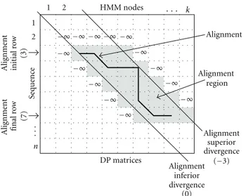
Given the DP matrices of the Viterbi algorithm, the limits of the best alignment are expressed by its initial and final rows and superior and inferior divergences (IR, FR, SD, and ID, resp.). The initial and final rows indicate the row of the matrices where the alignment starts and ends (initial and final element of the sequence involved in the alignment). The superior and inferior divergences represent how far the alignment departs from the main diagonal, in up and down directions, respectively. The main diagonal has divergence 0, the diagonal immediately above it has divergence −1, the next one −2, and so on. Analogously, the diagonals below the main diagonal have divergences +1, +2, and so on. These divergences are calculated as the difference i−j between the row (i) and column (j) coordinates of the matrix cell.Figure 3shows the main ideas behind the Plan7-Viterbi divergence algorithm.

HMM nodes Alig nment initial r o w (3) Alig nment final r o w (7) Sequenc e DP matrices Alignment inferior divergence (0) Alignment superior Alignment region Alignment 1 2 1

2 −∞ −∞ −∞ −∞ −∞

−∞ −∞ −∞ −∞ −∞ −∞ −∞ −∞ −∞ . . . n _divergence (−3)

· · · k

Figure _{3: Divergence concept: alignment limits, initialized cells}

(with−∞), and alignment region, for a HMM withk nodes and a sequence of lengthn.

determine what we define as the alignment region (AR), shown in shadow in the figure.

The AR contains the cells of the score matrices M, I, andDthat must be computed in order to obtain the best alignment. The other Viterbi algorithm DP vectors are also limited by IR and FR, as well. The alignment limits are calculated precisely, leaving no space to error, in a sense that computing only the cells inside the AR will produce the same best alignment as the unbounded (not limited to the AR) computation of the whole matrices.

The Plan7-Viterbi Divergence Algorithm (Plan7-Viterbi-DA) works in two main phases. The first phase is inserted into a simplified version of the Viterbi algorithm which eliminates data dependencies induced by theJstate. In this phase, we compute the similarity score of the best alignment of the sequence against the profile HMM, but we do not obtain the alignment itself. We also calculate the limits of the alignment, while computing the similarity score. These limits are computed as new DP matrices and vectors, by means of a new set of recurrence equations. The alignment limits IR, SD, and ID are computed for theM, I, D, E,andCstates. The FR limit is computed only for theCstate.

The Viterbi algorithm in (1) has the recurrence equation (2) for theMstate score computation:

M

i,j

=emMj,si + max ⎧ ⎪ ⎪ ⎪ ⎪ ⎪ ⎪ ⎪ ⎪ ⎨ ⎪ ⎪ ⎪ ⎪ ⎪ ⎪ ⎪ ⎪ ⎩ M

i−1,j−1

+ trMj−1,Mj

I

i−1,j−1

+ trIj−1,Mj

D

i−1,j−1

+ trDj−1,Mj

B(i−1) + trBi−1,Mj

.

(2)

Let SelM assume the values 0, 1, 2 or 3, depending on

the result of the maximum operator in (2). If the argument selected by the maximum operator is the first, second, third,

or fourth one, then SelM will assume the value 0, 1, 2, or

3, respectively. Then, the alignment limits IR, SD, and ID, concerning the score matrixM, are defined by the recurrence equations in (6).

Recurrence equations for the alignment limits IR, SD, and ID, concerning the score matrixM, for 1≤ i ≤nand 1≤j≤k:

IRMi,j= ⎧ ⎪ ⎪ ⎪ ⎪ ⎪ ⎪ ⎪ ⎪ ⎨ ⎪ ⎪ ⎪ ⎪ ⎪ ⎪ ⎪ ⎪ ⎩

IRMi−1,j−1, if SelM=0

IRIi−1,j−1, if SelM=1

IRDi−1,j−1, if SelM=2

i, if SelM=3,

SDMi,j= ⎧ ⎪ ⎪ ⎪ ⎪ ⎪ ⎪ ⎪ ⎪ ⎨ ⎪ ⎪ ⎪ ⎪ ⎪ ⎪ ⎪ ⎪ ⎩

SDMi−1,j−1, if SelM=0

min

i−j, SDIi−1,j−1, if SelM=1

min

i−j, SDD

i−1,j−1

, if SelM=2

i−j, if SelM=3,

IDMi,j= ⎧ ⎪ ⎪ ⎪ ⎪ ⎪ ⎪ ⎪ ⎪ ⎨ ⎪ ⎪ ⎪ ⎪ ⎪ ⎪ ⎪ ⎪ ⎩

IDMi−1,j−1, if SelM=0

max

i−j, IDIi−1,j−1, if SelM=1

max

i−j, IDDi−1,j−1, if SelM=2

i−j, if SelM=3.

(3)

The alignment limits IR, SD, and ID, related to the score matrices I and D and vector E, are defined analogously, based on the value of SelI, SelD, and SelE, determined

by the result of the maximum operator of the Viterbi algorithm recurrence equation for the I, D, and E states, respectively. Given the recurrence equation for theCstate’s score computation in the Viterbi algorithm in (1), let SelC

assume the values 0 or 1, depending on the result of the maximum operator in this equation. Equation (4) shows the recurrence equations that define the alignment limits IR, FR, SD, and ID, concerning theCscore vector.

The first phase of the Plan7-Viterbi-DA was thought to be implemented in hardware because its implementation in software would increase the memory requirements and processing time as it introduces new DP matrices. Besides, the Divergence values computation does not create new data dependencies inside the Viterbi algorithm and can be performed in parallel to the similarity score calculation.

The second phase of the Plan7-Viterbi-DA uses the output data coming from the first one (similarity score and divergence values). If the alignment’s similarity score is significant enough, then the second phase generates the alignment. To do this the software executes the Viterbi algorithm again for that sequence.

Divergence algorithm

Phase 1 Alignment

score and limits computation

(In hardware) (In software) Alignment

limits HMMs

Sequences Alignment

Phase 2 Alignment

score1 Alignment

score2

Alignment generation (only if score1

significant)

Figure_{4: Phases of the Plan7-Viterbi-DA.}

the high-level structure of the Plan7-Viterbi-DA and the interaction between its two phases.

Recurrence equations for the alignment limits IR, FR, SD, and ID, concerning theCscore vector, for 1≤i≤n:

IRC(i)= ⎧ ⎨

⎩

IRC(i−1), if SelC=0

IRE(i), if SelC=1,

FRC(i)= ⎧ ⎨

⎩

FRC(i−1), if SelC=0

i, if SelC=1,

SDC(i)= ⎧ ⎨

⎩

SDC(i−1), if SelC=0

SDE(i), if SelC=1,

IDC(i)= ⎧ ⎨

⎩

IDC(i−1), if SelC=0

IDE(i), if SelC=1.

(4)

The Plan7-Viterbi-DA’s second phase is implemented in software as a modification inside HMMER’s Viterbi function used by the hmmpfam and hmmsearch programs. In this function, we need to initialize with −∞ only the cells immediately above, to the left and to the right of the AR, as shown inFigure 3. The main loops are also modified in order to calculate only the cells inside the AR, using the alignment limits IR, FR, SD, and ID.

In the next section we propose a hardware implementa-tion of the first phase of Plan7-Viterbi-DA.

5. HMMER-ViTDiV Architecture

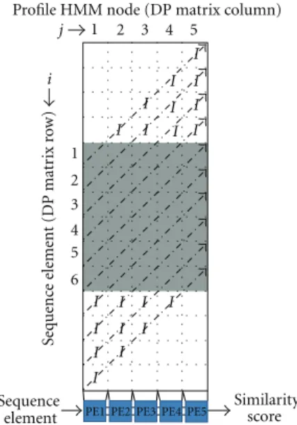
The proposed architecture, called HMMER-ViTDiV, consists of an array of interconnected processing elements (PEs) that implements a simplified version of the Viterbi algo-rithm, including the necessary modifications to calculate the Plan7-Viterbi-DA presented inSection 4. The architecture is designed to be integrated to the system as a pre-filter stage that returns the similarity score and the alignment limits for a query sequence with a specific profile HMM. If the similarity score for the query sequence is significant enough, then the software uses the alignment limits calculated for the sequence inside the architecture and generates the alignment using the Plan7-Viterbi-DA. Each PE calculates the score for the jcolumn of the DP matrices of the Viterbi algorithm and the alignment limits for the same column.Figure 5shows the DP matrices antidiagonals and their relationship with each one of the PEs when the number of profile HMM nodes is equal

Sequence element

Profile HMM node (DP matrix column)

I I I I

I I I I I I

I I I I I I I I I I

Sequenc

e element (DP mat

rix r

o

w)

1

2 3 4 5

6

1 2 3 4 5

j

Similarity score i

PE1 PE2 PE3 PE4 PE5

Figure _{5: PE to DP matrices correspondence when the HMM}

number of nodes is less or equal to the number of PEs.

to the number of implemented PEs inside the architecture. In the figure, the arrows show the DP matrices anti-diagonals, cells marked with I correspond to idle PEs, and shaded cells correspond to DP cells that are being calculated by their corresponding PE. The systolic array is filled gradually as the sequence elements are inserted until there are no idle PEs left, and then, when sequence elements are exiting, it empties until there are no more DP cells to calculate.

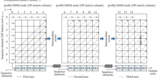
Since the size of commercial FPGAs is currently limited, today we cannot implement a system with a number of PEs that is equal to one of the largest profile HMM in sequence databases (2295) [2]. We implemented a system that divides the computation into various passes, each one computing a band of sizeNof the DP matrices, whereNis the maximum number of PEs that fits into the target FPGA. In each pass the entire sequence is fed across the array of PEs and the scores are calculated for the current band. Then the output of the last PE of the array is stored inside FIFOs, as it is the input to the next pass and will be consumed by the first PE.Figure 6 presents the concept of band division and multiple passes.

As shown in Figure 6, in each pass the PE acts as a different node of the profile HMM and has to be loaded with the corresponding transition and emission probabilities that are required by the calculations. Also, we note that the system does not have to wait for the entire sequence to be out of the array in one pass to start the next pass, and the PEs can be in different passes at a given time.

Two RAM memories per PE are included inside the architecture to store and provide the transition and emission probabilities for all passes. Two special sequence elements are included in the design to ease the identification of the end of a pass (@) and the end of the sequence processing (∗_{). A controller is implemented inside each PE to identify}

profile HMM node (DP matrix column)

Sequenc

e element (DP mat

rix r

o

w)

In

te

rm

ediat

e

sc

or

es

Sequence

elements _{First pass Second pass Third pass}

profile HMM node (DP matrix column) profile HMM node (DP matrix column)

In

te

rm

ediat

e

sc

or

es

Sequence

elements Sequence elements

Id

le P

Es

1

2

3

4

5

6

7 0

0 1 2 3 4 5 6 7 8 9 10 11 12 13 14

Output score j

PE1 PE2 PE3 PE4 PE5 PE1 PE2 PE3 PE4 PE5 PE1 PE2 PE3 PE4 PE5

i

−∞ −∞ −∞ −∞ −∞ −∞ −∞ −∞ −∞ −∞ −∞ −∞ −∞ −∞ −∞

−∞

−∞

−∞

−∞

−∞

−∞

−∞

FIFO FIFO

Total profile HMM nodes: 13 Computation passes (bands): 3

Figure_{6: PE to DP matrices correspondence for HMMs with more nodes than the number of PEs (band division and multiple passes).}

Emission RAM

Transition RAM

Emission RAM

Transition RAM

reg bank

Transition Transition

reg bank

Transition reg bank

Inputs

Pass

Score stage Score stage Score stage

Control signals Control signals Control signals Divergence stage Divergence stage Divergence stage

PE 1 PE 2

Intermediate result FIFOs (score and divergences)

B vector unit

C vector unit

Outputs

Emission RAM

Transition RAM

PEn

Figure_{7: Block diagram of the accelerator architecture.}

An input multiplexer had to be included to choose between initialization data for the first pass and intermediate data coming from the FIFOs for the other passes.

A transition register bank had also to be included to store the 9 transition probabilities used concurrently by the PE. This bank is loaded in 5 clock cycles by a small controller inside the transition block RAM memory.Figure 7shows a general diagram of the architecture.

As illustrated inFigure 7, the PE consists of a score stage which calculates the M, I, D, and E scores and a Plan7-Viterbi divergence stage which calculates the alignment limits for the current sequence. Additional modules are included for theBandCscore vector calculations which were placed outside the PE array in order to have an easily modifiable and homogeneous design.

5.1. Score Stage. This stage calculates the scores for theM,I, D,andEstates of the simplified Viterbi algorithm (without theJ state). Each PE represents an individual HMM node, and calculates the scores as each element of the sequence

passes through. The PE’s inputs are the scores calculated for the current element in a previous HMM node, and the PE’s outputs are the scores for the current sequence element in the current node. The score stage of the PE uses (a) 16-bit saturated adders which detect and avoid overflow or underflow errors by saturating the result either to 32767 or to−32768 and (b) modified maximum units which not only return the maximum of its inputs but also the index of which of them was chosen. Finally, the score stage consists also of 8 16-bit registers used to store the data required by the DP algorithm to calculate the next cell of the matrix. Figure 8shows the operator diagram of the score stage. The 4-input maximum unit was implemented in parallel in order to reduce the critical path of the system and thus increase the operating frequency.

M(i,j−1) tr(M j−1,M j)

B(i) I(i,j−1)

D(i,j−1)

E(i,j−1)

tr(I j−1,M j)

tr(Dj−1,M j)

tr(Mj−1,Dj)

tr(Dj−1,Dj)

M(i−1,j)

I(i−1,j)

D(i−1,j)

E(i−1,j) +

+

+ +

+

+

+

+

+

+ +

Ma

x

Ma

x

Ma

x

Ma

x

tr(M j,E)

SelM

SelI

SelD

SelE

tr(B,M j)

tr(Mj,Ij) tr(Ij,Ij) B(i−1)

Figure_{8: Score stage for the architecture’s PE.}

the calculated alignment limits for the current element. The outputs depend directly on the score stage of the PE and are controlled by the SelM, SelI, SelD,and SelE signals. The

divergence stage also requires the current sequence element index, in order to calculate the alignment limits. Figure 9 shows the Plan7-Viterbi-DA implementation for theMand Estates.

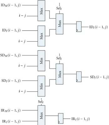
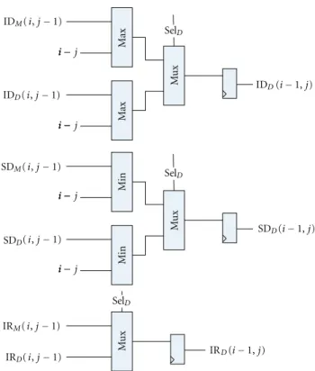
Figures 10 and 11 show the Plan7-Viterbi-DA imple-mentation for the I and Dstates, respectively. The Base J parameter is the position of the PE in the systolic array, and the #PE parameter is the total number of PEs in the current system implementation. These parameters are used to initialize the divergence stage registers according to the current pass and ensure that the limits are calculated correctly. The divergence stage is composed of (a) 2 input maximum and minimum operators, (b) 4 and 2 input multiplexers, in which the selection lines are connected to the control signals coming from the score stage, and (c) 16-bit registers, which serve as temporal storage for the DP data that is needed to calculate the current divergence DP cell.

5.3. B and C Score Vector Calculation Units. The B score Vector calculation unit is in charge of feeding the PE array with the Bscore values. This module is placed left of the first PE, and it is connected to the B(i−1) input of it. It has to be initialized for the first iteration with the tr(N,B) transition probability for the current profile HMM by the control software. For other iterations, it adds the tr(N,N) probability to the previous values and feeds the output to the

first PE. As discussed in Sections2and4, the Plan7-Viterbi-DA does not generate modifications to theBcalculation unit. Figure 12shows its hardware implementation.

The Ccalculation unit is in charge of consuming theE output provided by the last PE of the array and generating the output similarity score for the current element of the query sequence (the score for the best alignment up to this sequence element). Since the Plan7-Viterbi-DA introduces the calculation of the limits for the best alignment in this state of the Viterbi algorithm, the score stage of theCunit also delivers the control signal (SelC) for the multiplexers of

the divergence stage.Figure 13shows theCstate calculation unit, including the score and divergence stages.

6. Proposed Performance Measurement

#PE _Base

j

Pass

Ma

x

Ma

x

Mi

n

Mi

n

Mu

x

Mu

x

Mu

x

Mu

x

Mu

x

Mu

x

+ −

i

i− i−j i−j

i− i−j

i− i

i

−j

i− i−j i−

i− i−j

i− i− i− i−j IDM(i,j−1)

IDI(i,j−1)

IDD(i,j−1)

IDE(i,j−1)

SDM

SDI

SDD

SDE

(i,j−1)

(i,j−1)

(i,j−1)

(i,j−1)

IRM(i,j−1)

IRI(i,j−1)

IRD(i,j−1)

IRE(i,j−1)

SelM

SelE

SelM

SelE

SelM

SelE

iout

IDM(i−1,j)

IDE(i−1,j)

SDM(i−1,j)

SDE(i−1,j)

IRM(i−1,j)

IRE(i−1,j) ×

Figure_{9: Divergence calculating stage forMandEstates.}

The second approach measures the execution times of the unaccelerated software when executing a predefined set of sequence comparisons. Then compares it to the execution time of the accelerated system when executing the same set of experiments, to obtain the real gain when integrating a hardware accelerator and the Plan7-Viterbi-DA.

LetStbe the total number of query sequences in the test

set,Ptthe total number of profile HMMs in the test set,ts(i,j) the time the unacceleratedhmmsearchtakes to compare the

query sequenceSi to the profile HMMPj,trep(i,j) the time the Plan7-Viterbi-DA takes to reprocess the significant query sequenceSiand the profile HMMPj,tcon(i,j) the time spent in communication and control tasks inside the accelerated system, andth(i,j)the time the hardware accelerator takes to execute the comparison between the query sequenceSiand

the profile HMMPj.

IDM(i−1,j)

IDI(i−1,j) IDI(i−1,j)

SDM(i−1,j)

SDI(i−1,j)

SDI(i−1,j)

IRM(i−1,j)

IRI(i−1,j) IRI(i−1,j)

Ma

x

Ma

x

Mi

n

Mi

n

Mu

x

Mu

x

Mu

x

i− i−j

i− i−j

i− i−j

i− i−j

SelI

SelI

SelI

Figure_{10:Istate divergence calculating stage.}

accelerated system (Tsa), and the achieved performance gains

(G). The timests(i,j),th(i,j),trep(i,j), andtcon(i,j) are obtained directly from HMMER, the implemented accelerator, and the software implementing the Plan7-Viterbi-DA and will be shown in the following sections:

Tss←− St

i=1

Pt

j=1

ts(i,j), (5)

Tsa←− St

i=1

Pt

j=1

th(i,j)+trep(i,j)+tcon(i,j)

, (6)

G←− Tss

Tsa. (7)

7. Experimental Results

The proposed architecture not only enhances software execution by applying a pre-filter to the HMMER software but also provides a means to limit the area of the DP matrices that needs to be reprocessed, by software, in the case of significant sequences. Because of this, the speedup of the solution must be measured by taking into account the performance achieved by the hardware pre-filter as well as the saved software processing time by only recalculating the scores inside the alignment region. Execution time is measured separately for the hardware by measuring its real throughput rate (including loading time and interpass delays) and for software by computing the savings when calculating the scores and the alignment of the divergence-limited region of the DP matrices (Figure 3).

Experimental tests were conducted over all the 10340 profile HMMs for the PFam-A protein database [2]. Searches were made using 4 sets of 2000 randomly sampled protein sequences from the UniProtKB/SwissProt protein database [1] and only significantly scoring sequences were considered to be reprocessed in software. To find out which sequences from the sequence set were significant, we utilized a user-defined threshold and relaxed it to include the greatest possible number of sequences [11]. The experiments were done several times to guarantee the repeatability of them and the stability of the obtained data.

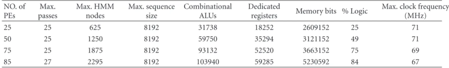
7.1. Implementation and Synthesis Results. The complete system was implemented in VHDL and mapped to an Altera Stratix II EP2S180F1508C3 device. Several configurations were explored to maximize the number of HMM nodes, the number of PEs, and the maximum sequence length. In order to do design space exploration, we developed a parameterizable VHDL code, in which we can modify the PE word size, the number of PEs of the array, and the size of the memories.

For the current implementation, we obtained a max-imum frequency of 67 MHz after constraining the design time requirements in the Quartus II tool to optimize the synthesis for speed instead of area. Further works will include pipelining the PE to achieve better performance in terms of clock frequency.Table 3 shows the synthesized configurations and their resource utilization.

IDM(i,j−1)

IDD(i,j−1)

SDM

SDD

(i,j−1)

(i,j−1)

IRM(i,j−1)

IRD(i,j−1)

Ma

x

Ma

x

Mi

n

Mi

n

Mu

x

Mu

x

Mu

x

i− i− i−j

i− i− i−j

i− i− i−j

i− i− i−j

SelD

SelD

SelD

IDD(i−1,j)

SDD(i−1,j)

IRD(i−1,j)

Figure_{11:Dstate divergence calculating stage.}

tr(N,B)

Load

B(i) tr(N,N)

+

Figure_{12:Bscore vector calculation unit (seeSection 2).}

tr(C,C) +

+ tr(E,C)

Score stage

Divergence stage

Ma

x

Mu

x

Mu

x

Mu

x

Mu

x

E(i,k)

IDE(i,k) SDE(i

i ,k)

IRE(i,k)

IDCout SDCout

FRCout

IRCout

SelC

SelC SelC

SelC

SelC

Cout

Table_{3: Area and performance synthesis results.}

NO. of PEs

Max. passes

Max. HMM nodes

Max. sequence size

Combinational ALUs

Dedicated

registers Memory bits % Logic

Max. clock frequency (MHz)

25 25 625 8192 31738 18252 2609152 25 71

50 25 1250 8192 59750 35294 3121152 49 71

75 25 1875 8192 93132 52520 3663152 75 69

85 27 2295 8192 103940 59285 5230592 84 67

hmmsearch

ex

ecution times (s)

Total execution time

execution time

Estimated execution times (regression results) TraceBack routine execution time hmmsearchexecution times versus DP cells

Plan 7-Viterbi routine

sequence elements (DP cells) 80

70

60

50

40

30

20

10

0

−10

0 2 4 6 8 10 12 14 16 ×108

profileHMM node number∗

Figure_{14: Unacceleratedhmmsearchperformance for the test set.}

we used a platform composed of an Intel Centrino Duo processor running at 1.8 GHz, 4 GB of RAM memory, and a 250 GB hard drive. HMMER was compiled to optimize execution time inside a Kubuntu Linux distribution. We also modified the hmmsearch program in order to obtain the execution times only for the Viterbi algorithm, as it was our main target for acceleration.

The characterization of HMMER was done by executing the entire set of tests (4 sets of 2000 randomly sampled sequences compared against 10340 profile HMMs) in the modifiedhmmsearchprogram. This was done to obtain an exact measure of the execution times of the unaccelerated software and to make its characterization when executing in our test platform.Figure 14shows the obtained results for the experiments.

The line with triangular markers represents the total execution time of the hmmsearch program including the alignment generation times, the line with circular markers represents the execution time only for the Viterbi algorithm, the line with square markers represents the time consumed by the program when generating the alignments, and the line with the plus sign markers corresponds to the expected execution times obtained via the characterization expression shown in (8).

Letlibe the number of amino acids in sequenceSi and

letmjbe the number of nodes in the profile HMMPj. Then

the time to make the comparison between the profile HMM and the query sequence (ts(i,j)) was found to be accurately represented by (8) which was found by making a least-squares regression on the data plotted in the circle-marked line ofFigure 14:

ts(i,j)←− −1.3684∗10−18

mjli 2

+ 4.3208∗10−8

∗mjli

−0.1160.

(8)

Even though we ran our tests with all the profile HMMs in the PFam-A database [2], we chose to show results only for 6 representative profile HMMs that include the smallest and the largest of the database, due to space limitations.Table 4 shows the estimated execution time obtained with (8) and its error percentage when compared to the actually measured execution times. We can calculate the number of average cell updates per second (CUPS) as the total number of elements of the entire data set sequences times the number of nodes of the profiles in the set divided by the complete execution time of the processing. We obtained a performance of 23.157 mega-CUPS for HMMER executing on the test platform.

7.3. Hardware Performance. We formulated an equation for performance prediction of the proposed accelerator, taking into account the possible delays, including systolic array data filling and consuming, profile HMM probabilities loading into RAM memories, and probability reloading delays when switching between passes. In order to validate the equation’s results, we developed a test bench to execute all the test sets. I/O data transmission delays from/to the PC host were not considered into the formula due to the fact that, in platforms such as the XD2000i [23], data transmission rates are well above the maximum required for the system (130 MBps).

Let mi be the number of nodes of the current HMM,

Sj the size of the current query sequence being processed,

nthe number of PEs in hardware, f the maximum system frequency,Thw the throughput of the system (measured in

CUPS), and th(i,j)the time the accelerator takes to process one sequence set. Then Thw and th(i,j) are fully described by (9) and (10), where 25n⌈mi/n⌉are the number of cycles

spent loading the current HMM into memory,nare the array filling number of cycles, (Sj+ 6)⌈mi/n⌉are the cycles spent

Table_{4: Modifiedhmmsearchperformance results.}

Sequence set elements Number of HMM

nodes Measured time (total)

Measured time (Viterbi only)

Estimated time

(Viterbi only) Error (%)

687406

788 23.40 23.28 22.871 1.75

10 0.40 0.35 0.1810 48.2

226 6.55 6.47 6.5635 1.42

337 9.85 9.8 9.8199 0.2

2295 74.49 64.09 64.6425 0.8

901 26.32 26.25 26.1199 0.4

697407

788 24.34 23.48 23.2158 1.12

10 0.47 0.41 0.1853 54.1

226 6.68 6.66 6.6602 0.003

337 9.88 9.83 9.9634 1.35

2295 78.87 62.89 65.5334 4.2

901 27.55 25.96 26.4938 2.05

700218

788 24.40 23.37 23.3082 0.264

10 0.42 0.38 0.1865 50.92

226 6.76 6.72 6.6873 0.486

337 10.26 9.84 10.0037 1.663

2295 81.23 62.25 65.7849 5.678

901 27.41 26.33 26.5989 1.021

712734

788 25.42 24.03 23.7193 1.293

10 0.42 0.37 0.1919 48.13

226 6.82 6.77 6.8083 0.565

337 10.09 10.01 10.1832 1.730

2295 81.07 63.81 66.8985 4.840

901 27.46 26.82 27.0665 0.919

∗

Execution times are all expressed in seconds.

that the unaccelerated algorithm will have to calculate to process the current sequence with the current HMM:

Thw

=

#Seqs i=1

#HMMs

j=1 Simj

#HMMs

j=1

#Seqs

i=1 (Si+ 6)

mj/n

+ 25nmj/n

+n−2

∗f,

(9)

th(i,j)= (Si+ 6)

mj/n

+ 25nmj/n

+n−2

f . (10)

We made the performance evaluation for the 4 proposed systolic PE arrays (25, 50, 75, and 85 PEs) and found out that the two characteristics that greatly influence the performance of the array are the quantity of PEs implemented in the array and the number of nodes of the profile HMM we are comparing the sequences against.

Table 5shows the obtained performances for all the array variations when executing the comparisons for our 4 sets of sequences against the 6 profile HMM subsets. The best result for each case is shown in bold. From the table we can see that performance increases significantly with the number of

implemented PEs. Also we can observe that the system has better performance for profile HMMs whose node number is an exact multiple of the array node number. This is due to the fact that, when a PE does not correspond to a node inside the profile HMM, its transition and emission probabilities are set to minus infinity in order to stop that PE to modify the previously calculated result and only forward that result, thus wasting a clock cycle and affecting performance.

Figures15and16show the variations in the accelerator performance with the implemented PE number and the profile HMM node number, as seen from the experimental results.

From Figure 16 we can see that, as the performance varies according with profile HMM node number, there is an envelope curve around the performance data which shows the maximum and minimum performances of the array when varying the number of the HMM nodes.

Table_{5: Hardware performance results.}

Sequence set elements

Number of HMM nodes

25 PEs 50 PEs 75 PEs 85 PEs

Thw

(GCUPS) th(sec)

Thw

(GCUPS) th(sec)

Thw

(GCUPS) th(sec)

Thw

(GCUPS) th(sec)

687406

788 1.7468 0.3101 3.4903 0.1552 4.9293 0.1068 5.4203 0.0971 10 0.7093 0.0097 0.7086 0.0097 0.6880 0.0097 0.6877 0.0097 226 1.6031 0.0969 3.2033 0.0485 3.8876 0.0388 5.1815 0.0291 337 1.7075 0.1357 3.4118 0.0679 4.6377 0.0485 5.7949 0.0388

2295 1.7695 0.8915 3.5358 0.4462 5.0942 0.3010 5.8468 0.2622

901 1.7274 0.3586 3.3607 0.1843 4.7691 0.1262 5.6341 0.1068

697407

788 1.7468 0.3146 3.4904 0.1574 4.9295 0.1083 5.4205 0.0985 10 0.7093 0.0098 0.7086 0.0098 0.6880 0.0099 0.6877 0.0099 226 1.6031 0.0983 3.2033 0.0492 3.8878 0.0394 5.1817 0.0296 337 1.7075 0.1376 3.4119 0.0689 4.6379 0.0492 5.7952 0.0394

2295 1.7695 0.9045 3.5359 0.4527 5.0944 0.3053 5.8471 0.2660

901 1.7274 0.3638 3.3608 0.1870 4.7693 0.1280 5.6344 0.1084

700218

788 1.7468 0.3159 3.4905 0.1581 4.9296 0.1088 5.4206 0.0989 10 0.7093 0.0099 0.7086 0.0099 0.6880 0.0099 0.6877 0.0099 226 1.6031 0.0987 3.2034 0.0494 3.8878 0.0396 5.1818 0.0297 337 1.7075 0.1382 3.4120 0.0692 4.6379 0.0494 5.7953 0.0396

2295 1.7695 0.9081 3.5359 0.4545 5.0945 0.3066 5.8472 0.2671

901 1.7274 0.3652 3.3608 0.1877 4.7693 0.1286 5.6345 0.1088

712734

788 1.7468 0.3215 3.4906 0.1609 4.9298 0.1107 5.4209 0.1007 10 0.7093 0.0100 0.7086 0.0101 0.6880 0.0101 0.6878 0.0101 226 1.6031 0.1005 3.2035 0.0503 3.8880 0.0403 5.1821 0.0302 337 1.7075 0.1407 3.4121 0.0704 4.6382 0.0503 5.7956 0.0403

2295 1.7695 0.9244 3.5360 0.4626 5.0947 0.3120 5.8475 0.2719

901 1.7274 0.3718 3.3609 0.1911 4.7696 0.1308 5.6348 0.1108

A

cc

eler

at

o

r per

for

manc

e (GCUPS)

Number of implemented PEs

Profile HMM with

Performance versus PE number

10 nodes 226 nodes 337 nodes

788 nodes 901 nodes 2295 nodes 6

5

4

3

2

1

0

20 30 40 50 60 70 80 90

Figure_{15: Performance versus number of PEs relation.}

A

cc

eler

at

o

r per

for

manc

e (GCUPS)

ProfileHMM node number

Array with

Accelerator performance versus ProfileHMM node number

25 PEs 50 PEs

75 PEs 85 PEs 6

5

4

3

2

1

0

0 500 1000 1500 2000 2500

Figure_{16: Performance versus number of HMM nodes envelope}

Table_{6: Second-stage performance estimations.}

Sequence set elements Number of HMM nodes

Entire sequence set processing time in unaccelerated HMMER (sec)

Significant sequences reprocessing time with prefilter and unaccelerated

HMMER (sec)

Divergence accelerated significant sequences reprocessing time (sec)

687406

788 23.40 0.234 0.0515

10 0.40 0.004 0.0009

226 6.55 0.0655 0.0144

337 9.85 0.0985 0.0217

2295 74.49 0.7449 0.1639

901 26.32 0.2632 0.0579

697407

788 24.34 0.2434 0.0535

10 0.47 0.0047 0.001

226 6.68 0.0668 0.0147

337 9.88 0.0988 0.0217

2295 78.87 0.7887 0.1735

901 27.55 0.2755 0.0606

700218

788 24.40 0.244 0.0537

10 0.42 0.0042 0.0009

226 6.76 0.0676 0.0149

337 10.26 0.1026 0.0226

2295 81.23 0.8123 0.1787

901 27.41 0.2741 0.0603

712734

788 25.42 0.2542 0.0559

10 0.42 0.0042 0.0009

226 6.82 0.0682 0.015

337 10.09 0.1009 0.0222

2295 81.07 0.8107 0.1784

901 27.46 0.2746 0.0604

an estimate of the performance of the second stage, we made a study in which we executed the comparison of the 20 top profile HMMs from the PFam-A [2] database with our 4 sets of query sequences to obtain both the similarity score and the divergence data for them. Then we built a graph plotting the similarity score threshold and the number of sequences with a similarity score greater than the threshold. From this graph we learned that less than 1% of the sequences were considered significant, even relaxing the threshold to include very bad alignments. With this information, we plotted the percentage of the DP matrices that the second stage of the system will have to reprocess in order to find out the worst case situation and make our estimations based on it. FromFigure 17 we can see that, for the experimental data considered, in the worst case the divergence region only corresponds to 22% of the DP matrices.

To obtain the second-stage performance estimations for HMMER (trep(i,j) in (6)), we obtained the percentage of significant sequences (ps), multiplied it by the worst case

percentage of the DP matrices that the second stage has to reprocess in order to generate the alignment (pc), and

then we multiplied it by the time the program hmmsearch takes to do the whole query sequence (Si) comparison with

a profile HMM (Pj). Equation (8) shows the expression

used to estimate the performance for the second stage. Table 6 presents the obtained results and also shows the comparison between the times the second stage will spend reprocessing the significant sequences with and without the Plan7-Viterbi-DA. As shown inTable 6, we obtained a performance gain up to 5 times only in the reprocessing stage.

t(reg(i,j))=t∗ps∗pc (11)

Table_{7: Total system performance and obtained performance gains.}

Sequence set elements

Number of HMM nodes

Prefilter hardware execution time (sec)

Divergence second-stage execution time (sec)

Total time (tsa(i,j))

Unaccelerated HMMER execution

time (sec)

Obtained gain

687406

788 0.0971 0.0515 0.1486 23.40 157.4697

10 0.0097 0.0009 0.0106 0.40 37.7358

226 0.0291 0.0144 0.0435 6.55 150.5747

337 0.0388 0.0217 0.0605 9.85 162.8099

2295 0.2622 0.1639 0.4261 74.49 174.8181

901 0.1068 0.0579 0.1647 26.32 159.8057

697407

788 0.0985 0.0535 0.152 24.34 160.1316

10 0.0099 0.001 0.0109 0.47 43.1193

226 0.0296 0.0147 0.0443 6.68 150.7901

337 0.0394 0.0217 0.0611 9.88 161.7021

2295 0.2660 0.1735 0.4395 78.87 179.4539

901 0.1084 0.0606 0.169 27.55 163.0178

700218

788 0.0989 0.0537 0.1526 24.40 159.8952

10 0.0099 0.0009 0.0108 0.42 38.8889

226 0.0297 0.0149 0.0446 6.76 151.5695

337 0.0396 0.0226 0.0622 10.26 164.9518

2295 0.2671 0.1787 0.4458 81.23 182.2118

901 0.1088 0.0603 0.1691 27.41 162.0934

712734

788 0.1007 0.0559 0.1566 25.42 162.3244

10 0.0101 0.0009 0.011 0.42 38.1818

226 0.0302 0.015 0.0452 6.82 150.885

337 0.0403 0.0222 0.0625 10.09 161.44

2295 0.2719 0.1784 0.4503 81.07 180.0355

901 0.1108 0.0604 0.1712 27.46 160.3972

Significant sequences/1000

DP matrices percentage needing to be reprocessed Similarity score threshold

25

20

15

10

5

0

−2 −1 0 1 2 3 4 ×105

Table_{8: Related work and comparison with our solution.}

Reference Number of_PEs Max. number of_{HMM nodes} Max. sequence_size

Complete Plan7-Viterbi

algorithm

Clock (MHz) Performance_(GCUPS) Gain FPGA

[3] 68 544 1024 N 180 10 190 Xilinx Virtex II 6000

[13] 90 1440 1024 N 100 9 247 Xilinx 2VP100

[11] 50 — — N 200 5 to 20 — Not Synthesized

[14] 72 1440 8192 N 74 3.95 195 XC2V6000

[15] 10 256 — Y 70 7 300 XC3S1500

[16] 50 — — N 66 1.3 50 Xilinx Spartan 3 4000

[20] 25 — — Y 130 3.2 56.8 Xilinx Virtex 5 110-T

Our work 85 2295 8192 N 67 5.8 254

(182∗₎

Altera Stratix II EP2S180F1508C3

∗

Including significant sequences reprocessing times.

shows the obtained performance gains. The table presents a summary of the execution time for each individual part of the system and calculates the performance gains with respect to the unaccelerated HMMER by applying (6).

Table 8 shows a brief comparison of this work with the ones found in the literature. We support longest test sequences and bigger profiles when compared with most works. As we include the divergence stage, we have to pay an area penalty, which limit the maximum number of PEs when compared with [13] and can affect the performance of the system. Nevertheless, we obtain additional gains from the divergence, a fact that justify the area overhead. Our architecture performs worse than complete Viterbi implementations such as the one presented in [15], but these cases are uncommon, and even if we relax the threshold for a sequence to be considered significant, the inclusion of the accelerator yields significant speedup.

8. Conclusions

In this paper, we introduced the Plan7-Viterbi-DA that enables the implementation of a hardware accelerator for the hmmsearchandhmmpfamprograms of the HMMER suite. We proposed an accelerator architecture which acts as a pre-filtering phase and uses the Plan7-Viterbi-DA to avoid the full reprocessing of the sequence in software. We also intro-duced a more accurate performance measurement strategy when evaluating HMMER hardware accelerators, which not only includes the time spent on the pre-filtering phase or the hardware throughput but also includes reprocessing times for the significant sequences found in the process.

We implemented our accelerator in VHDL, obtaining performance gains of up to 182 times the performance of the HMMER software. We also made a comparison of the present work with those found in the literature and found that, despite the increased area, we managed to fit a considerable amount of PEs inside the FPGA, which are capable of comparing query sequences with even the largest profile HMM present in the PFam-A database.

For future works we intend to adapt the Plan7-Viterbi-DA to a complete version of the Plan7-Viterbi algorithm

(including theJ state) and make a pipelined version of the PE architecture, in order to further increase the performance gains achieved when integrating the array with the HMMER software.

Acknowledgments

The authors would like to acknowledge the CNPq, the National Microelectronics Program (PNM), the FINEP, the Brazilian Millennium Institute (NAMITEC), the CAPES, and the Fundect-MS for funding this work.

References

[1] The Universal Protein Resource—UniProt, June 2009,http:// www.uniprot.org/.

[2] Sanger’s Institute PFAM Protein Sequence Database, May 2009,http://pfam.sanger.ac.uk/.

[3] A. C. Jacob, J. M. Lancaster, J. D. Buhler, and R. D. Chamber-lain, “Preliminary results in accelerating profile HMM search on FPGAs,” inProceedings of the 21st International Parallel and Distributed Processing Symposium, (IPDPS ’07), Long Beach, Calif, USA, March 2007.

[4] “HMMER: biosequence analysis using profile hidden Markov models,” 2006,http://hmmer.janelia.org/.

[5] R. Durbin, S. Eddy, A. Krogh, and G. Mitchison, Biological Sequence Analysis Probabilistic Models of Proteins and Nucleic Acids, Cambridge University Press, New York, NY, USA, 2008. [6] R. Darole, J. P. Walters, and V. Chaudhary, “Improving MPI-HMMER’s scalability with parallel I/O,” Tech. Rep. 2008-11, Department of Computer Science and Engineering, University of Buffalo, Buffalo, NY, USA, 2008.

[7] G. Chukkapalli, C. Guda, and S. Subramaniam, “SledgeHM-MER: a web server for batch searching the Pfam database,”

Nucleic Acids Research, vol. 32, supplement 2, pp. W542– W544, 2004.

[8] “HMMER on the sun grid project,” July 2009,http://www.psc .edu/general/software/packages/hmmer/.

[9] D. R. Horn, M. Houston, and P. Hanrahan, “ClawHMMER: a streaming HMMer-search implementation,” inProceedings of the ACM/IEEE Supercomputing Conference, (SC ’05), Novem-ber 2005.

[10] GPU-HMMER, July 2009,

[11] R. P. Maddimsetty, J. Buhler, R. D. Chamberlain, M. A. Franklin, and B. Harris, “Accelerator design for protein sequence HMM search,” in Proceedings of the 20th Annual International Conference on Supercomputing (ICS ’06), pp. 288–296, New York, NY, USA, July 2006.

[12] “BLAST: Basic Local Alignment Search Tool,” September 2009,

http://blast.ncbi.nlm.nih.gov/.

[13] K. Benkrid, P. Velentzas, and S. Kasap, “A high performance reconfigurable core for motif searching using profile HMM,” inProcedings of the NASA/ESA Conference on Adaptive Hard-ware and Systems (AHS ’08), pp. 285–292, Noordwijk, The Netherlands, June 2008.

[14] T. F. Oliver, B. Schmidt, Y. Jakop, and D. L. Maskell, “High speed biological sequence analysis with hidden Markov models on reconfigurable platforms,”IEEE Transactions on Information Technology in Biomedicine, vol. 13, no. 5, pp. 740– 746, 2009.

[15] J. P. Walters, X. Meng, V. Chaudhary et al., “MPI-HMMER-boost: distributed FPGA acceleration,”Journal of VLSI Signal Processing Systems, vol. 48, no. 3, pp. 223–238, 2007.

[16] S. Derrien and P. Quinton, “Parallelizing HMMER for hard-ware acceleration on FPGAs,” inProceedings of the Interna-tional Conference on Application-specific Systems, Architectures and Processors (ASAP ’07), pp. 10–17, Montreal, Canada, July 2007.

[17] L. Hunter,Artificial Intelligence and Molecular Biology, MIT Press, 1st edition, 1993.

[18] D. Gusfield,Algorithms on Strings, Trees and Sequences: Com-puter Science and Computational Biology, Cambridge Univer-sity Press, 1997.

[19] L. R. Rabiner, “A tutorial on hidden Markov models and selected applications in speech recognition,”Proceedings of the IEEE, vol. 77, no. 2, pp. 257–286, 1989.

[20] Y. Sun, P. Li, G. Gu et al., “HMMer acceleration using systolic array based reconfigurable architecture,” inProceedings of the ACM/SIGDA International Symposium on Field Programmable Gate Arrays (FPGA ’09), p. 282, New York, NY, USA, May 2009. [21] T. Takagi and T. Maruyama, “Accelerating hmmer search using FPGA,” inProceedings of the19th International Conference on Field Programmable Logic and Applications (FPL ’09), pp. 332– 337, Prague Czech Republic, September 2009.

[22] R. B. Batista, A. Boukerche, and A. C. M. A. de Melo, “A parallel strategy for biological sequence alignment in restricted memory space,”Journal of Parallel and Distributed Computing, vol. 68, no. 4, pp. 548–561, 2008.