Ant´
onio Manuel Passos Eleut´
erio
Licenciado em Ciˆencias da Engenharia Electrot´ecnica e de Computadores
2D Position System for a Mobile Robot in
Unstructured Environments
Disserta¸c˜ao apresentada para obten¸c˜ao do Grau de Mestre em Engenharia Electrot´ecnica e de Computadores, pela Universidade Nova
de Lisboa, Faculdade de Ciˆencias e Tecnologia.
Orientador : Fernando Coito, Professor Associado, FCT-UNL
J´uri:
Presidente: Anik´o da Costa, Professora Auxiliar, FCT-UNL Arguente: Paulo Gil, Professor Auxiliar, FCT-UNL
Vogal: Fernando Coito, Professor Associado, FCT-UNL
i
2D Position System for a Mobile Robot in Unstructured Environments
Copyright ➞Ant´onio Manuel Passos Eleut´erio, Faculdade de Ciˆencias e Tecnologia, Uni-versidade Nova de Lisboa
Acknowledgements
I would like to thank to professor Paulo Oliveira and Carlos Cardeira for the guid-ance and suggestion of this dissertation theme. A very interesting and challenging theme covering various study areas, that contributed to my knowledge growth.
I express my gratitude to my advisor Fernando Coito for his wise advising towards scientific knowledge. All meetings I had with him were very instructive, making me realize difference perspectives of knowledge. Without him this dissertation quality would be inferior.
Prof. Lu´ıs Palma was not officially an advisor or supervisor. However, he was always available to an interesting chat, providing support and advices, related to my dissertation, scientific matters, finding a job matters, or other cultural matters, and sometimes even leisure matters. I am grateful to him for all this companionship.
Thank you to all my friends from FCT-UNL. In special, Jo˜ao Pires for his constant support and friendship throughout this degree. My flatmates Carlos Raposo and F´abio Querido for their support in my bad mood times, for their companionship, studying and growing up together. And Jos´e Vieira for his friendship and encouraging me in critical times.
Finally, I would like to show my special gratitude to my family, that provided me support and education to surpass this stage of life.
Resumo
Hoje em dia, existem v´arios sensores e mecanismos para estimar a trajet´oria e lo-caliza¸c˜ao de um robˆo m´ovel, relativamente ao seu meio de navega¸c˜ao. Normalmente os mecanismos de posicionamento absoluto s˜ao os mais precisos, mas tamb´em s˜ao os mais caros, e requerem equipamento pr´e-instalado, exterior ao robˆo. Portanto, um sistema capaz de medir o seu movimento e localiza¸c˜ao relativamente ao seu meio de navega¸c˜ao (posicionamento relativo) tem sido uma ´area de investiga¸c˜ao fulcral desde o in´ıcio do aparecimento dos ve´ıculos aut´onomos. Com o aumento do desempenho computacional, o processamento da vis˜ao por computador tem-se tornado mais r´apido e, portanto, tor-nado poss´ıvel incorpor´a-la num robˆo m´ovel. Em abordagens, baseadas em marcadores, de odometria visual, a estima¸c˜ao de modelos implica a ausˆencia total de falsas associa¸c˜oes de marcadores (outliers) para se ter uma correta estima¸c˜ao. A rejei¸c˜ao de outliers ´e um processo delicado, tendo em conta que existe sempre um compromisso entre a velocidade e fiabilidade do sistema.
Esta disserta¸c˜ao prop˜oe um sistema de posi¸c˜ao 2D, para uso interior, usando odome-tria visual. O robˆo m´ovel tem uma cˆamera apontada ao teto, para a an´alise de imagem. Como requisitos, o teto e ch˜ao (onde o robˆo se move) devem ser planos. Na literatura, o RANSAC ´e um m´etodo muito usado para a rejei¸c˜ao deoutliers. No entanto, pode ser lento em circunstˆancias cr´ıtica. Por conseguinte, ´e proposto um novo algoritmo que acelera o RANSAC, mantendo a sua fiabilidade. O algoritmo, chamado FMBF, consiste na com-para¸c˜ao de padr˜oes de textura entre as imagens, preservando os padr˜oes mais parecidos. Existem v´arios tipos de compara¸c˜ao, com differentes custos e fiabilidade computacional. O FMBF gere estas compara¸c˜oes, a fim de otimizar o compromisso entre velocidade e fiabilidade.
Palavras Chave: Odometria Visual,RANdom SAmple Consensus (RANSAC),
Feature Metrics Best Fit (FMBF), Marcadores.
Abstract
Nowadays, several sensors and mechanisms are available to estimate a mobile robot trajectory and location with respect to its surroundings. Usually absolute positioning mechanisms are the most accurate, but they also are the most expensive ones, and require pre installed equipment in the environment. Therefore, a system capable of measuring its motion and location within the environment (relative positioning) has been a research goal since the beginning of autonomous vehicles. With the increasing of the computa-tional performance, computer vision has become faster and, therefore, became possible to incorporate it in a mobile robot. In visual odometry feature based approaches, the model estimation requires absence of feature association outliers for an accurate motion. Outliers rejection is a delicate process considering there is always a trade-off between speed and reliability of the system.
This dissertation proposes an indoor 2D position system using Visual Odometry. The mobile robot has a camera pointed to the ceiling, for image analysis. As requirements, the ceiling and the floor (where the robot moves) must be planes. In the literature, RANSAC is a widely used method for outlier rejection. However, it might be slow in critical circumstances. Therefore, it is proposed a new algorithm that accelerates RANSAC, maintaining its reliability. The algorithm, called FMBF, consists on comparing image texture patterns between pictures, preserving the most similar ones. There are several types of comparisons, with different computational cost and reliability. FMBF manages those comparisons in order to optimize the trade-off between speed and reliability.
Keywords: Visual Odometry (VO), RANSAC, FMBF, Features.
List of Acronyms
AGV Automatic Guided Vehicle
AR Aspect Ratio
CS Corner Signature
CDS Corner Distance Signature
CTS Corner Triangle Signature
CTAS Corner Triangle Angle Signature
CTDS Corner Triangle Distance Signature
DOF Degrees of Freedom
DoG Difference of Gaussian
EKF Extended Kalman Filter
FAST Features from Accelerated Segment Test
FAST-ER FAST - Enhanced Repeatability
FMBF Feature Metrics Best Fit
FOV Field Of View
FPS Frames Per Second
GPS Global Positioning System
IMU Inertial Measurement Unit
LASER Light Amplification by Stimulated Emission of Radiation
NN Nearest Neighbour
RANSAC RANdom SAmple Consensus
SI International System of Units
SIFT Scale Invariant Feature Transformation
SLAM Simultaneous Localisation And Mapping
SUSAN Smallest Univalue Segment Assimilating Nucleus
VO Visual Odometry
VSLAM Visual SLAM
List of Symbols
a a pixel location of the arc A
A set of locations of the arc of ncontiguous pixels of the FAST segment test
b distance between the lens of the camera and the ceiling
b1 distance between the lens and the edge entrance of the camera
b2 distance between the edge entrance of the camera and the ceiling
B matrix of the quality values of the accepted corner matches
~
B ascendant sorted vector of the quality values of the accepted corner matches
BCS RANSAC best consensus set
BM RANSAC best model
CS RANSAC consensus set
C0:n set of robot poses, between 0 and n, in relation to the origin
Ck kth robot pose in relation to the origin
D a set of data matches used in RANSAC
DΘ,i,j set of differences between Θi and Θj
DΦ,i,j set of differences between Φi and Φj
Ek set of corner matches used for the estimation of the kth pose
F OV camera field of view
F OVw width camera field of view
F OVh height camera field of view
gw×h camera calibration factor for frames with resolution w×h
h frame height
Hk relative motion between the kth and thek−1th frame
Hα transformation between the central reference of Ik and the ceiling reference
Hβ transformation between the central reference of Ik−1 and the ceiling reference
I0:n set of frames between poses 0 and n
Ip intensity of corner p
Ip→l intensity of pixel p→l
Ik kth frame
It generic designation for number of iterations
It(N) number of iterations depending of the number of corners
l a location of the FAST circle segment test
L set of locations of the FAST circle segment test
L∆ number of corner triangle signatures used in corner metrics
n minimum size of p→A for a corner detection
N generic designation for the number of corners in a frame
Nask number of asked corners
Nf number of filtered corners in WCA
Nia number of points inside the intercepted area between frames ¯
Nα
ia number of points outside the intercepted area between frames
Nk number of corners in the kth frame
Nα number of corners in frame α
Nα,b number of bright corners in frame α
Nα,d number of dark corners in frame α
Nα,nr number of non repeated corners in frame α
Nα,r number of repeated corners in frame α
Nβ,b number of bright corners in frame β
Nβ,d number of dark corners in frame β
Nβ,nr number of non repeated corners in frame β
Nβ,r number of repeated corners in frame β
m a length of the image projection of the camera
M C number of corner match combinations
M Cbc best case of the number of corner match combinations
M Cwc worst case of the number of corner match combinations
M M RANSAC maybe model
Ma number of accepted corner matches
Me number of elected corner matches
Min number of corner match inliers
xiii
p generic corner designation
p→a a pixel of the arc p→A at locationa
p→A arc of n contiguous pixels of the FAST segment test
p→l a pixel of the FAST detector segment test at location l p→L all pixels of the FAST segment test
pk kth corner in a frame
pk,i,a corner athat belongs to theith triangle of the kth corner
pk,i,b corner bthat belongs to theith triangle of the kth corner
pα a corner in frame α
pβ a corner in frame β
P set of all pixels in a frame
Pb set of bright corners in a frame
Pd set of dark corners in a frame
Ps set of non corners in a frame
Pα
i coordinates of the ith point of frameα
Piβ coordinates of the ith point of frameβ
Q set of quick rejection locations of the FAST segment test
QCDS (quality) average of the differences between CDS
QCDS,i,j average of the differences between CDS, of ith andjth corners of frames α and β
p→Q set of pixels with locations Q
RP number of repeated points in corner signatures simulator
Rk relative rotation between the kth and thek−1th frame
sk kth distance of a CTS comparison
sα,i ith distance of Sα
sβ,j jth distance of Sβ
Sp→l state of the pixel p→lin relation to the candidate corner p
Sα set of corner distances in frame α
Sα,r set of repeated corner distances in frame α
Sβ set of corner distances in frame β
Sβ,r set of repeated corner distances in frame β
t generic designation of FAST detector threshold
tD minimum number of distance comparisons for the approval of a CDS comparison
tma limit number of approved comparisons in FMBF
tmax maximum threshold tnecessary to make a corner detectable
tmb limit of the number of accepted corner matches
tmd threshold value to determine if a corner fits a model in RANSAC
tk FAST detector threshold used in the kth frame
t∆ minimum neighbour distance to create a CTS
t∆s threshold used to reject CTS differences
tΘ threshold for a CTAS match validation
tΦ threshold for a CTDS match validation
Tk relative translation between the kth and thek−1th frame
w frame width
W generic designation for the set of corner coordinates in a frame
Wk set of corner coordinates in the kth frame
Wk,k−1 set of corner coordinates of the kth and thek−1
th frames
W′
k,k−1 set of filtered corner coordinates of the k
th and thek−1th frames
X x coordinate of the robot pose
Y y coordinate of the robot pose
Z z coordinate of the robot pose
α designation for previews frame
β designation for current frame
∆Ip→L set of colour intensity differences between pixel p and each pixel on p→L ∆Ip→A set of colour intensity differences between pixel p and each pixel on p→A ∆si,j difference between the distances sα,i and sβ,j
ηin inliers portion
ηin(N) inliers portion depending on the number of corners
ηout outliers portion
ηout(N) outliers portion depending on the number of corners
ηr generic designation for portion of repeated corners in a frame
ηα,r portion of repeated corners in frame α
ηβ,r portion of repeated corners in frame β Υk set of tmax values of thekth frame
θ robot orientation
xv
Θ set of amplitude angles of a CTS
Θi set of amplitude angles of a CTS of the ith corner, of frameα Θj set of amplitude angles of a CTS of the jth corner, of frameβ
ρ probability of selecting at least one sample with all inliers, after running RANSAC
υ minimum number of data matches to fit a model in RANSAC
φk,i,a distance between pk and pk,i,a
φk,i,b distance between pk and pk,i,b
Φ set of pairs of distances that creates a CTDS
Φi set of pairs of distances that creates a CTDS of the ith corner of frameα Φj set of pairs of distances that creates a CTDS of the jth corner of frameβ
ϕ angle of a rigid body rotation
Ωw×h relation between millimetre and pixel in a frame with resolution w×h Ω′
Contents
Acknowledgements iii
Resumo v
Abstract vii
List of Acronyms ix
List of Symbols xi
1 Introduction 1
1.1 Motivation . . . 1 1.2 Proposed System . . . 2 1.3 Objectives and Contributions . . . 2 1.4 Organization . . . 3
2 AGV Localisation 5
2.1 Simultaneous Localisation And Mapping (SLAM) . . . 5 2.2 Absolute and Relative Positioning . . . 8 2.3 Sensors and Techniques . . . 8 2.3.1 Odometry . . . 9 2.3.2 Inertial Measurement Unit . . . 10 2.3.3 Magnetic Compasses . . . 11 2.3.4 Active Beacons . . . 12 2.3.5 Visual Odometry . . . 13 2.3.5.1 The problem . . . 14 2.4 VO Motion Estimation . . . 16 2.5 Detecting and Matching Features . . . 17 2.6 Feature Detectors . . . 19 2.6.1 Moravec Corner Detector . . . 19 2.6.2 FAST Feature Detector . . . 20 2.7 Outlier removal . . . 22 2.7.1 RANSAC . . . 22
2.8 Summary . . . 24
3 Visual Odometry and Mapping 27
3.1 A Visual Odometry approach . . . 27 3.1.1 Introduction . . . 27 3.1.1.1 Context . . . 29 3.1.2 Picture frame capture . . . 31 3.1.3 FAST feature detection . . . 32 3.1.3.1 Frame resolution dependency . . . 36 3.1.4 Corner features pre-processing . . . 38 3.1.4.1 Corner Distance Signature . . . 39 3.1.4.2 Corner Triangle Signature . . . 40 3.1.5 Corner features matching . . . 41 3.1.5.1 RANSAC . . . 45 3.1.5.2 Feature Metrics Best Fit . . . 48 3.1.6 Motion estimation . . . 58 3.1.7 Process chain . . . 61 3.1.7.1 Choice of detecting a corner . . . 62 3.1.7.2 Controlling the number of corners . . . 63 3.1.7.3 Windowed Corner Adjustment . . . 64 3.2 Mapping . . . 66 3.3 Camera calibration . . . 67 3.4 Simulation . . . 71 3.4.1 Corner Signatures Simulator . . . 72 3.4.2 Picture Frames Simulator . . . 75 3.5 Summary . . . 79
4 Experimental results 81
4.1 Introduction . . . 81 4.2 FAST Detector time dependency . . . 81 4.3 Experiences . . . 83 4.3.1 Picture Map . . . 83 4.3.2 Frame Visual Odometry . . . 90 4.3.3 Video Mapping . . . 96 4.4 Error relation . . . 101 4.5 Summary . . . 104
5 Conclusions and Future Work 105
5.1 Conclusions . . . 105 5.2 Future Work . . . 106
List of Figures
2.1 Example of the SLAM problem. . . 6 2.2 Global reference and robot local reference. . . 9 2.3 6 DOF read by the IMU sensor. . . 11 2.4 Triangulation draft of the active beacons system. . . 12 2.5 Example of blobs detection. From [FS11]. . . 13 2.6 A block diagram showing the main components of a VO system. . . 15 2.7 Illustration of the VO problem. From [FS11]. . . 17 2.8 Example of feature matching between two frames. . . 18 2.9 FAST detection in an image patch. From [RD05] . . . 21 2.10 FAST detection in a frame. From [RD05] . . . 21 2.11 Estimated inliers of a data set contaminated with outliers. . . 23
3.1 Perspective view of the robot, performing a one dimension movement. . . . 28 3.2 Example of two successive picture frames taken to a certain ceiling. Top:
geometric dispersions of both frames of the ceiling. Bottom: collected frame data. . . 29 3.3 VO block diagram. . . 31 3.4 Perspective projection: scene plane (SI) and image plane (px) . . . 32 3.5 FAST feature detection in a frame patch. . . 33 3.6 Frame patch and the pixels with Qlocations. . . 33 3.7 Corner points extracted from FAST-9 with t = 22. Top: 108 corners.
Bottom: 165 corners. . . 34 3.8 Corner points extracted from FAST-9 with t = 18. Top: 222 corners.
Bottom: 375 corners. . . 35 3.9 The problem of disappearing corners between frames due to the robot motion. 36 3.10 Corner detection interfered by Gaussian noise and perspective rotation. In
b) a rotation is performed from a). . . 37 3.11 Influence of a perspective rotation in corner detection with high resolution.
In b) a rotation is performed from a). . . 38 3.12 Representation of a corner distance signature (blue lines). . . 39 3.13 Necessary iterations for the calculation of 7 corner distance signatures. . . . 40
3.14 Three angles of a corner triangle signature. . . 41 3.15 Abstract case of matches combinations. . . 41 3.16 Matches combinations divided by corner symmetry. . . 42 3.17 Correct intended corner matches. . . 42 3.18 Correct matches with non repeated corners. . . 43 3.19 Graph of the outliers portion in function of the corner number for different
repeatability. . . 45 3.20 Graph of the number of iterations in function of the number of corners. . . 48 3.21 Several discrete circles with different radius approximations. . . 50 3.22 An example that leads to a wrong CTS match: a) frame α, b) frame β. . . 50 3.23 Influence of a non repeated corner in CTS. . . 51 3.24 Correct matches with non repeated corners. . . 53 3.25 An example of CDS matching calculation. . . 54 3.26 Filtering of unfavourable differences. . . 55 3.27 Example of a conversion ofB toB~. . . 56 3.28 Trade-off between speed and efficiency of FMBF options. . . 57 3.29 Reference relation between a pair of frames. . . 60 3.30 Ceiling reference creation. . . 60 3.31 Ideal block diagram. . . 61 3.32 Determinetmax through ∆Ip→L. . . 62
3.33 Example of choosingtk+1 in Υk, using Nask. . . 63 3.34 Example of WCA filtering 3 pairs of sets Υk withNf = 12. . . 65 3.35 Block diagram with WCA. . . 65 3.36 Frame sequence taken from a ceiling. . . 66 3.37 Map performed by a frame sequence. . . 66 3.38 Field of view of the camera. . . 67 3.39 A calibration picture. . . 68 3.40 Calibration graph. . . 70 3.41 Millimetre per pixel in function of the distanceb2. . . 70 3.42 Geometry of both frames in a random example of a signature simulation. . 73 3.43 A signature simulation match. . . 74 3.44 Path selection option. . . 75 3.45 Locations and orientations of the virtual frames. . . 76 3.46 Virtual frame sequence. . . 76 3.47 Matching between frame 1 and 2. . . 77 3.48 Matching between frame 2 and 3. . . 77 3.49 Matching between frame 3 and 4. . . 77 3.50 Groundtruth and path estimation. . . 78
LIST OF FIGURES xxi
4.3 Graph of the number of detected corners per frame from test A. . . 85 4.4 Graph of the number of selected corners in frame α and β, of test A. . . 86 4.5 Graph of the relation between time and several frame match properties (A). 87 4.6 Graph of the RANSAC rejection in test A. . . 88 4.7 Geometry of the path performed by the robot in test A. . . 89 4.8 Map performed by the taken frames of the test A. . . 89 4.9 Picture of the Lab 1 ceiling. . . 90 4.10 Corner controller effect of testB. . . 91 4.11 Number of collected corners per match of testB. . . 92 4.12 Graph of the relation between time and several frame match properties (B). 93 4.13 Graph of the RANSAC rejection in testB . . . 93 4.14 Robot position graph analysis of testB. . . 94 4.15 Error of the absolute poses in testB. . . 94 4.16 Frame match between frames 14 and 15, of testB. . . 95 4.17 Map performed by the taken frames of testB. . . 95 4.18 Example of Close Corners problem. . . 97 4.19 Corner controller effect of test C. . . 98 4.20 RANSAC Rejection of test C. . . 99 4.21 Time consuming of the frame matches of test C. . . 99 4.22 Robot positions graph of test C. . . 100 4.23 Map performed by the taken frames of test C. . . 100 4.24 Graph of the error depending of the robot displacement and orientation,
between pairs of frames. . . 101 4.25 Graph of the error depending of the robot displacement for orientations
below 180◦
. . . 102 4.26 Graph of the error depending of the robot displacement for orientations
below 90◦
. . . 103 4.27 Graph of the error depending of the robot displacement for orientations
below 30◦
List of Tables
2.1 Time taken to perform a feature detection with FAST, SUSAN and Harris. From [RD05]. . . 22
3.1 Number of corners and matches of an artificial example. . . 43 3.2 Correspondence of 2 CDS. . . 53 3.3 A CDS match with unfavourable marriages. . . 55 3.4 Behaviour of the field of view. . . 69 3.5 Results of the corner signatures simulation. . . 74 3.6 Results of the picture frames simulation. . . 78
4.1 Input parameters of test A. . . 83 4.2 Number of detected corners in each frame, of test A. . . 84 4.3 Number of selected corners and corner match combinations of testA. . . 85 4.4 Frame match quality and time consuming of test A. . . 86 4.5 Frame match quality and time consuming of test A. . . 88 4.6 Results of the robot motion in test A. . . 88 4.7 Input parameters of the frame test B. . . 91 4.8 Input parameters common to the 5 parameter configurations. . . 96 4.9 Most important input parameters. . . 97 4.10 Failures and time results. . . 97
Chapter 1
Introduction
This chapter introduces the navigation and mapping systems for Automatic Guided Vehicle (AGV), based on the literature. An overview is performed about several sensors and techniques available to use in Simultaneous Localisation And Mapping (SLAM). The proposed system of the dissertation is revealed, using theVisual Odometry (VO) technique alone. The objectives and contributions are presented in order to solve the literature problems. An algorithm approach is proposed to make VO a faster process. Also, the structure of the dissertation is presented, organized by chapters.
1.1
Motivation
Mobile robot navigation and mapping has been a central research topic in the last few years. An autonomous mobile robot needs to track its path and locate its position rela-tive to the environment. Such a task is still a challenge when operating in unknown and unstructured environments. However, from a theoretical and conceptual point of view, it is now considered a solved problem. SLAM is a crucial method for the resolution of this problem. SLAM has the purpose of building a consistent map while simultaneously esti-mating the robot position within the map. SLAM may be designed for different domains such as to outdoor or indoor, to wheeled or legged, to underwater and to airborne systems. Furthermore, robots are built for different purposes, leading to a wide variety of navigation mechanisms. Therefore, the complexity of the surroundings and the way the robot inter-acts with the surroundings varies considerably. Due to current technology limits, there is
not a standard approach regarding this matter. In order to achieve SLAM, different types of sensors are used, contributing for the efficiency of the process. Combinations of sensors are chosen, according to the environment and robot tasks purposes.
Wheel odometry, Inertial Measurement Unit (IMU), magnetic compasses, active bea-cons, VO, are very common techniques associated with the estimation of a vehicle position and location. Nevertheless, when combining several sensors for that purpose, visual odom-etry is usually a favourite choice. The main reason is that VO is very versatile, considering it is not restricted to a particular locomotion method, and the relation between motion estimation accuracy and the system expense is very appealing.
1.2
Proposed System
This dissertation aims to implement an indoor 2D tracking position system for a mobile robot through a VO operation, using a single camera pointed upward to the ceiling. The robot motion is estimated through successive comparisons between picture frames of the ceiling. In each frame, several local patterns are detected, designated as landmarks or features. The consecutive frames need to have overlapped areas, where the features can be compared and matched. By matching features throughout the frame sequence, the robot motion of the last frame in relation to the first frame is estimated.
This system is limited to a 2D path. The ceiling has to be a plane as well as the floor where the robot moves. Running a VO system in real time is a major goal in the literature. The algorithm needs to be fast and reliable enough to accomplish real time. The most burdensome process is the feature matching between frames. Therefore, a new algorithm approach is implemented in this dissertation, which aims to reduce the computational cost of the feature matching process.
1.3
Objectives and Contributions
accu-1.4. ORGANIZATION 3
racy, but reducing the computational cost considerably. The features used are specifically designated as corners (described in section 2.3.5), detected by the algorithmFeatures from Accelerated Segment Test (FAST). Each corner is considered a special pixel, positioned in pixel coordinates. Therefore, every corner has a Corner Signature (CS) which consists in all distances to the other corners of the same frame. Also, with two corner neighbours of a certain corner, aCorner Triangle Signature (CTS) is created. It is required a certain num-ber of CS comparisons with a high similarity to have a frame match. Therefore, instead of comparing all CS of one frame to all CS of the other frame, the CS comparisons run until such number of comparisons with high similarity is achieved. Additionally, for each corner comparison a CS comparison is performed only if a CTS inexpensive comparison is approved. For corner matches quick rejection, a pre corner filtering is performed in pairs of frames, before the feature matching, based on a corner detection parameter (designated as FAST threshold). Also, in order to have an appropriate number of corner detections per frame, a corner controller is presented, based on the last used FAST threshold and number of detected corners.
The work developed in this dissertation, led to a paper presented in an international conference, [CECV14].
1.4
Organization
This dissertation is organized as follows.
Chapter 1 introduces the navigation and mapping systems for AGV, based on the literature. An overview is performed about SLAM and several sensors and techniques used for it. It is revealed the proposed system of the dissertation, using the VO technique alone, and its constraints. The objectives and contributions are presented in order to solve the literature problems. It is proposed an algorithm approach to make VO faster. Also, the structure of the dissertation is presented, organized by chapters.
compar-isons are performed. Several VO techniques presented in the literature are explained and mentioned where they belong in the VO block diagram. Feature detection, feature match-ing and outlier removal are explained in detail and presented their importance to the success of a VO process.
Chapter 3 presents the VO solution proposed in this dissertation. It describes the camera projection that takes picture frames and justifies why the limited resolution of the frame. The FAST corner detector is detailed explained along with the differences between several FAST-n, varying n. After detecting the corners in one frame, it is explained how corner signatures are created in order to allow the corner matching between frames. RANSAC used alone for corner matching would bring a high temporal complexity, as stated. Therefore, the FMBF is carefully detailed in order to prove the reduction of such complexity. Using the frames, a map is performed throughout the trajectory. It is also mentioned how the camera calibration was performed, using several pictures taken to a certain plane. And also, the two simulators used to validate the FMBF algorithm are detailed.
Chapter 4 illustrates the experimental results of three particular tests. In the first test, nine frames of the same ceiling are used to build a map. In the second test, twenty four pictures of an other ceiling are used to estimate the robot path. In the third test, a video is used to create a map, based on where the robot went through.
Chapter 2
AGV Localisation
This chapter contains a literature review about mobile robotics position systems. An overview about several sensors and techniques used in SLAM is performed. The sensors are divided in absolute and relative positioning types, and comparisons are performed between them. In each sensor the benefits and inconvenients are highlighted and several comparisons are shown. It is explained several VO techniques presented in the literature and mentioned where they belong in the VO block diagram. Feature detection, feature matching and outlier removal are detailed and presented their relevance to the success of a VO process.
2.1
Simultaneous Localisation And Mapping
(SLAM)
The probabilistic SLAM problem was firstly proposed in the 1986 IEEE Robotics and Automation Conference held in San Francisco. A discussion between many researchers led to the recognition that a consistent probabilistic mapping was a fundamental problem in robotics with major conceptual and computational issues that needed to be addressed [DwB06]. In [SSC87, DW87] was established the statistical basis for describing relation-ships between landmarks and manipulating geometric uncertainty. Those works had the purpose of showing that there is a high degree of correlation between the estimates of the location of different landmarks in a map, and that these correlations grow with successive observations. Several results, regarding this issue, were demonstrated in visual navigation [AF88] and sonar-based navigation using Kalman filter type algorithms [CL85, Cro89].
Therefore, the solution for localisation and mapping required a joint state composed of the vehicle pose (i.e., position and orientation) and every landmark position, to be updated following each landmark observation [SSC87]. Currently that is how SLAM is performed. In SLAM the mobile robot can build a map of an environment and at the same time use the map to determine its location. Both the trajectory of the robot and the location of all landmarks are estimated online and without any location awareness in advance. Figure 2.1 illustrates an example SLAM draft.
Figure 2.1: Example of the SLAM problem.
In the figure a mobile robot moves across an environment taking relative observations of a number of landmarks using a sensor located on the robot. At time instant k the following quantities are defined:
1. xk: state vector of the location and orientation of the vehicle.
2. uk: control vector, applied at timek−1 to drive the vehicle to state xk at time k.
3. mi: vector describing the location of theithlandmark whose true location is assumed time invariant.
2.1. SIMULTANEOUS LOCALISATION AND MAPPING (SLAM) 7
to the discussion, or there are multiple landmark observations at a timek.
The following sets are also defined:
1. X0:k={x0, x1, ..., xk}={X0:k−1, xk}: History of the vehicle locations.
2. U0:k={u1, u2, ..., uk}={U0:k−1, uk}: History of control inputs.
3. m={m1, m2, ..., mn}: Set of all landmarks.
4. Z0:k={z1, z2, ..., zk}={Z0:k−1, zk}: Set of all landmark observations.
SLAM requires the probability distribution P(xk, m|Z0:k, U0:k, x0) to be computed for all k times. This probability distribution describes the joint posterior density of the landmark locations and the vehicle state, at time k, through the recorded observations and control inputs from the start until time k, and the initial state of the vehicle.
A recursive solution is used to the SLAM problem [DwB06]. It starts with an esti-mation of P(xk−1, m|Z0:k−1, U0:k−1) at timek−1, where the joint posterior is computed
using Bayes Theorem, following a control uk and an observation zk. This computation requires a state transition model and an observation model, describing the effect to the control input and observation respectively.
The most common representation for these models is in the form of a state-space model with additive Gaussian noise, leading to the use the Extended Kalman Filter (EKF).
The motion model of the vehicle can then be described in terms of a probability distribution of state transitions in the form of:
P(xk|xk−1, uk) :xk=f(xk−1, uk) +wk, (2.1)
where f(.) models vehicle kinematics and where wk are additive, zero mean uncorrelated Gaussian motion disturbances with covariance Qk.
Theobservation modeldescribes the probability of making an observationzk when the vehicle location and landmark locations are known, and is described in the form:
whereh(.) describes the geometry of the observation and wherevkare additive, zero mean uncorrelated Gaussian observation errors with covariance Rk.
2.2
Absolute and Relative Positioning
There are two basic position estimation methods, absolute and relative positioning, for a mobile robot. If possible, they are usually employed together for better reliability [BK87, SCDE95]. Relative positioning is based on monitoring robot poses, computing the offset from a known starting position. Absolute positioning methods rely on systems external to the robot mechanisms. They can be implemented by a variety of methods and sensors, but all of them present relevant inconvenients. For example, navigation beacons and landmarks have a significant accuracy, but require costly installations and maintenance. Or map-matching methods, also very accurate, are usually slow, preventing general commercial applications. Therefore, with these measurements it is necessary for the work environment either be prepared or be known and mapped with high precision [BKP92].
GPS can be used only outdoors and has a poor accuracy of 10 to 30 meters for non military devices. Such limitation is imposed by the US government deliberately, through small errors in timing and satellite position to prevent a hostile nation from using GPS in support of precision weapons delivery.
2.3
Sensors and Techniques
There is a wide variety of sensors and techniques for mobile robot positioning:
1. Classical odometry (wheeled), where the number of wheel revolutions is monitored;
2. IMU, which measures acceleration and orientation;
3. Magnetic compasses, that measures the Earth magnetic field;
4. Active beacons, which uses triangulation and trilateration;
2.3. SENSORS AND TECHNIQUES 9
6. LASER, which analyses scanned features.
Nevertheless, only the first five methods are worth devoting some attention for the background of this work.
2.3.1 Odometry
Odometry is one of the most used positioning systems for mobile robots. It is inex-pensive, accurate in short term and allows high sampling rates. The principle operation of odometry is the aggregation of incremental motion information over time. The vehi-cle localisation is estimated by calculating the performed displacement from the initial position. Due to the incremental nature of this measure type, the measure uncertainty increases over time [BEFW97]. In particular, orientation errors cause significant lateral errors, which grow proportionally with the distance traveled by the robot. With time those errors may become so large that the estimated robot position is completely wrong after 10 m of travel [GT94]. Nevertheless, most researchers invest in odometry considering that navigation tasks could be simplified by improving the odometric accuracy. For example, in order to obtain more reliable position estimations, [SD+99] and [GT94] propose fusing odometric data with absolute position measurements, mentioned previously.
Odometry is based on simple equations, which translates wheel revolutions into robot linear displacement relative to the floor, in order to provide the robot local reference relative to the global reference, as illustrated in figure 2.2.
However, wheel slippage may prevent the proportional translation into linear motion, among other smaller causes. There are two types of errors to consider, designated as systematic and non-systematic [Bor96]. Systematic errors result from kinematic imper-fections of the robot, such as, differences in wheel diameters or uncertainty associated with the exact wheelbase. Non-systematic errors result from the interaction of the wheels with the floor, such as, wheel slippage or bumps and cracks. In [Bor96] a method, called UMBmark, was designed to measure odometry systematic errors. UMBmark requires that the mobile robot follows an experience with stipulated conditions, in order to obtain a numeric value that expresses the odometric accuracy. In addition, similar to the latter, the extended UMBmark method was designed to measure non-systematic errors. In both cases, a calibration procedure was developed to reject or reduce odometry errors, providing a more reliable odometry process.
2.3.2 Inertial Measurement Unit
IMU is also an option when it comes to estimate a mobile robot position. It uses gyroscopes and accelerometers to measure rate of rotation and acceleration, respectively [BEFW97]. IMU systems have the advantage of being independent from external refer-ences. However, they have other serious disadvantages, as show in [BDW95] and [BDw94]. Studies found that there is a very poor signal-to-noise ratio at lower accelerations. Mea-surements need to be integrated twice, for accelerometers, to obtain the position, which makes these sensors extremely sensitive to drift. Also, they are sensitive to uneven ground. If there is a small disturbance in a perfectly horizontal position, the sensor detects a com-ponent of the gravitational acceleration g, adding more error to the system.
Gyroscopes provide information related to the rate of rotation of a vehicle only, which means their data need to be integrated once. They are more accurate than accelerometers, but also more costly. Gyroscopes can help compensate the foremost weakness of odometry, that is, large lateral position error. Small momentary orientation errors cause a constantly growing lateral position error. Therefore, detecting and correcting immediately orientation errors would be of great benefit.
2.3. SENSORS AND TECHNIQUES 11
Figure 2.3: 6 DOF read by the IMU sensor.
2.3.3 Magnetic Compasses
A magnetic compass is a sensor that provides a measure of absolute heading. This is important in solving navigation needs for mobile robots, considering there are no accu-mulated dead-reckoning errors. However, one unavoidable disadvantage of any magnetic compass is that the Earth magnetic field is often distorted near steel structures [BKP92] or power lines. For this reason, these sensors are not reliable for indoor applications.
2.3.4 Active Beacons
Active beacons are widely used for ships and airplanes, as well as on commercial mobile robotic systems. This navigation system provides accurate positioning information with minimal processing, as active beacons can be easily detected. It results that this approach stands high sampling rates with high reliability, but the cost of installation and maintenance is also very high. There are two different types of active beacon systems: trilateration and triangulation [BEFW97].
Trilateration is based on distance measurements to calculate the beacon sources, which leads to the estimation of the vehicle position. Usually there are three or more transmitters mounted at known locations in the environment and a receiver on board the vehicle. In reverse, there may be receivers mounted in the environment and one transmitter on board the vehicle. The famous Global Positioning System (GPS) is a particular trilateration example.
In triangulation there are three or more active transmitters mounted in know locations, as in trilateration. However, instead of estimating the position of the robot using the distances between transmitters and receiver, it uses the angles αk ∈ {α1, α2, α3}between the sensor and the three longitudinal axis, performed between the transmitters Tk ∈ {T1, T2, T3} and the sensor S. The sensor keeps on rotating on board, and registers the three angles. From these three measurements the robot coordinates and orientation can be computed. Figure 2.4 illustrates the draft of the triangulation active beacon type.
2.3. SENSORS AND TECHNIQUES 13
2.3.5 Visual Odometry
Nowadays, computer vision is an important application to mobile robotics. SLAM has often been performed using other sensors rather than regular cameras. However, recent improvements in both sensors and computing hardware have made real-time vision processing much more practical for SLAM applications, as computer vision algorithms mature. Furthermore, cameras are inexpensive and provide high information bandwidth, serving as cheap and precise localisation sensor.
The term VO was created in 2004 by Nist´er in his landmark paper [NNB04]. This term was chosen due to its similarity to wheel odometry. VO operates by successively estimate the pose of the vehicle through examination of the changes that motion induces on the images of its onboard cameras. A stereo head or a single camera may be used. As requirements, there should be sufficient illumination in the environment and a static scene with enough texture to allow apparent motion to be extracted. This system aims to construct the trajectory of the vehicle with no prior knowledge of the scene nor the motion for the pose estimation (relative positioning system). Consecutive picture frames should be captured by ensuring that they have sufficient scene overlap. VO works by detecting features (also named as keypoints or interest points) in the frames and matching them over overlapping areas from consecutive frames. The feature detection is usually performed with features such as corners or blobs. Figure 2.5 illustrates an example of blobs detection.
The feature matching may be performed by matching features in pairs of frames, or tracking features throughout several frames.
VO is not restricted to a particular locomotion method. It can be used in any robot with sufficiently high quality camera [FS11]. Compared to wheeled odometry, it has no slippage problems in uneven terrain or other adverse conditions. Nevertheless, outdoor terrains is in some way more challenging than indoor environments. Outdoors are un-structured, and simpler features such as corners, planes and lines that are abundant in indoor environments rarely exist in natural environments [AK07].
There is no ideal and unique VO solution for every possible working environment. The optimal solution should be chosen accurately according to the specific navigation and the given computational resources. Furthermore, many approaches use VO in conjunction with information from other sources such as GPS, inertia sensors, wheel encoders, among others [CECV14, How08, MCM07, KCS11]. Over the three decades of VO history, only in the third decade real-time flourished, which has led this system to be used on another planet by two Mars exploration rovers for the first time. In Mars, rovers used IMU and wheeled encoder-based odometry that performed well within the design goal of at most 10% error. However, the rover vehicles were also driven along slippery slopes tilted as high as 31 degrees. In such conditions VO was employed to maintain a sufficiently accurate onboard position estimation [Mai05].
In [AK07] an approach using VO, IMU and GPS was used in rough terrain, accom-plishing localisations over several hundreds of meters within 1% of error.
In [NNB04] it is described a real-time method for deriving vehicle motion from monoc-ular and stereo video sequences, in autonomous ground vehicles. Obstacle detection and mapping is performed using visual input in stereo data, as well as, estimating the motion of the platform in real-time.
2.3.5.1 The problem
2.3. SENSORS AND TECHNIQUES 15
Moravec corner detector, and for presenting the first motion estimation pipeline, whose main functioning blocks are still used today. Figure 2.6 presents that pipeline for a VO system.
Figure 2.6: A block diagram showing the main components of a VO system.
The image sequence can be stereo or monocular. Moravec used monocular for Mars rovers. His VO system performed a 3D motion estimation with 6 Degrees of Freedom (DOF), equipped with what he termed as a slider stereo: a single camera sliding on a rail. The robot moved in a stop-and-go fashion, digitizing images and analysing them using extracted corners. Corners were detected in the images by his operator. The motion was then computed through a rigid body transformation to align the triangulated 3D points seen at two consecutive robot positions [FS11].
Most of the research done in VO has been produced using stereo cameras. Superior results were demonstrated in trajectory recovery for a planetary rover, due to absolute scale possession [MS87].
that windowed bundle adjustment can decrease the final position error by a factor of 2-5 on ranges up to 10km, in a VO experiment. Loop closure implies realizing when the robot returns to a previously visited area. This approach is more common in Visual SLAM (VSLAM), considering it is necessary to keep track of the map landmarks, in order to recognize a visited area.
2.4
VO Motion Estimation
In the case of a monocular system, the set of images taken at time k is denoted by
I0:n = {I0, ..., In}. In the case of a stereo system, there are a left and a right image at every time instant, denoted by Il,0:n = {Il,0, ..., Il,n} and Ir,0:n = {Ir,0, ..., Ir,n}. For simplicity, the camera coordinate is assumed to be also the robot coordinate. Two camera positions at adjacent time instantsk−1 andkare related by the rigid body transformation
Hk,k−1 ∈ ℜ4 ×4
of the following form:
Hk,k−1 =
Rk,k−1 Tk,k−1
0 1
, (2.3)
where Rk,k−1 ∈ ℜ3 ×3
is the rotation matrix, and Tk,k−1 ∈ ℜ3 ×1
the translation vector. The set H1:n = {H1,0, ..., Hn:n−1} contains all subsequent motions. Camera poses are
C0:n = {C0, ..., Cn}, containing the transformations of the camera with respect to the initial coordinate frame at k= 0. The current poseCn is computed by concatenating all the transformations Hk,k−1(k= 1, ..., n), and therefore, Ck=Ck−1Hk,k−1, whereas C0 is
the camera pose at the instant k= 0, which can be set arbitrarily by the user.
VO aims to compute the relative transformationsHk,k−1 from the imagesIk andIk−1,
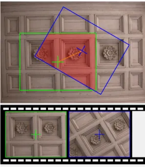
and then to concatenate the transformations in order to recover the full trajectory C0,n of the camera [FS11]. Figure 2.7 illustrates an example of the VO problem with stereo camera.
2.5. DETECTING AND MATCHING FEATURES 17
Figure 2.7: Illustration of the VO problem. From [FS11].
2.5
Detecting and Matching Features
Besides feature based methods, to compute the relative motion Hk,k−1, may also be
used appearance based methods, and hybrid methods. Appearance based methods use the intensity information of all the pixels in two input image (or subregion). A known example of this method is using all the pixels in two images to compute the relative motion using a harmonic Fourier transform [MGD07]. This method has the advantage of working with low texture, but it is computationally extremely expensive. Hybrid methods use a combination of the other two.
In feature detection, the image is searched for salient keypoints that are likely to match well in other images. Point detectors, such as corners of blobs, are important for VO because of their accurate positioning measurements in the image. A blob is an image pattern different from its immediate neighbourhood in intensity, colour, and texture.
matching), and invariance (to illumination, rotation, scale and perspective distortion). To accomplish feature matching (or tracking), features are characterized by a set of metrics, named feature descriptor. For example, the simplest descriptor of a feature is its appearance (i.e., the intensity of the pixels in a path around the feature point).
The simplest way for matching features between two frames is to compare all fea-ture descriptors from one frame with all feafea-ture descriptors from the other frame. Such comparisons are performed by similarity between pairs of feature descriptors. However, exhaustive matching becomes quadratic with the number of features, which is computa-tionally expensive, and could became impractical when the number of features is large. Other feature matching methods like multidimensional tree search or hash table could be used [BL97]. Figure 2.8 illustrates an example of feature matching in two frames.
Figure 2.8: Example of feature matching between two frames.
In the example the camera poses are in samples k and k−1, the features are of type fi and fi′, the corresponding points in the environment are of type pi, and the pose transformation isHk,k−1 (i∈ {1,2,3,4,5}).
2.6. FEATURE DETECTORS 19
in the first image and search for their corresponding matches in the following images. This method is suitable for situations when the amount of motion and appearance deformation between adjacent frames is small. However, the features can suffer from large changes in long images sequences, providing a bad outcome [FS11].
2.6
Feature Detectors
In the VO literature there are many point feature detectors. The most common corners detectors are: Moravec [Mor80], F¨orstner [FG87], Harris [HS88], Shi-Tomasi [ST94], and FAST [RD05]. And the most common blob detectors are: SIFT [TW09], SURF [BTG06], and CENSURE [AKB08]. Here is performed an overview of Moravec and Harris, which have been widely used in VO applications, and FAST that is used in this work. Although FAST is not the most robust in 3D localization, the literature claims this feature detector is currently the fastest one, among the other corner detectors [FS12]. Therefore, FAST is chosen for this work due to its speed, and due to the fact that this work aims to accomplish 2D localization. With 2D localization, significantly less complex than 3D, there is not a significant difference in the corner detectors in terms of robustness.
2.6.1 Moravec Corner Detector
Moravec operator is considered a corner detector, since it defines interest points as points where there is a large intensity variation in every direction. The concept ”point of interest” as distinct regions in images was defined by Moravec. In his work, it was concluded that to find matching regions in consecutive image frames, these interest points could be used. This proved to be a vital low level processing step in determining the existence and location of objects in the vehicle environment [Mor80].
The Moravec corner detector algorithm is stated below. The input parameters of this algorithm are:
I - Grayscale image;
w(x, y) - Binary window;
The output parameter of this algorithm is:
C - Cornerness map.
Input :I,w(x, y), T Output:C
foreach pixel (x,y) in I, do
// Calculate the itensity variation from shifts (u, v) of: // (1,0),(1,1),(0,1),(−1,1),(−1,0),(−1,−1),(0,−1),(1,−1)
Vu,v(x, y) =P x,y
w(x, y)[I(x+u, y+v)−I(x, y)]2
// Calculate the cornerness map
C(x, y) =min(Vu,v(x, y))
// Threshold the interest map
if C(x, y)< T then C(x, y) = 0
Perform non-maximal suppression toC // To find local maxima // All the remaining non-zero points in C are corners.
Algorithm 2.1:Moravec.
Harris corner detector [HS88] was developed as a successor of Moravec corner detector. The difference lies on a Gaussian window w(x, y) = exp(−x22+σ2y2), instead of a binary
window vulnerable to noise, and in the use of a the Taylor expansion to compute all shifts, instead of using a set of shifts at every 45 degree. Results proved Harris to be more efficient and robust to noise [HS88, DNB+12].
2.6.2 FAST Feature Detector
It is stated that the FAST detector is sufficiently fast allowing online operation of the tracking system [RD05]. In order to detect a corner, a test is performed at a pixel p by examining a circle of 16 pixels (a Bresenham circle of radius 3) surrounding p. A corner is detected atp if the intensities of at least 12 contiguous pixels are all above or all below the intensity of p by some thresholdt. This is illustrated in figure 2.9.
2.6. FEATURE DETECTORS 21
Figure 2.9: FAST detection in an image patch. From [RD05]
are brighter than C by more than the threshold.
The test of this condition is optimized by examining pixels 1, 9, 5 and 13, to reject candidate pixels more quickly, considering a corner exists only if three of these test points are all above or below the intensity of pby the threshold.
A corner is categorized as positive, where the intensities of the contiguous pixels of the segment test are greater that the intensity of the pixel in the centre, and negative, on the contrary.
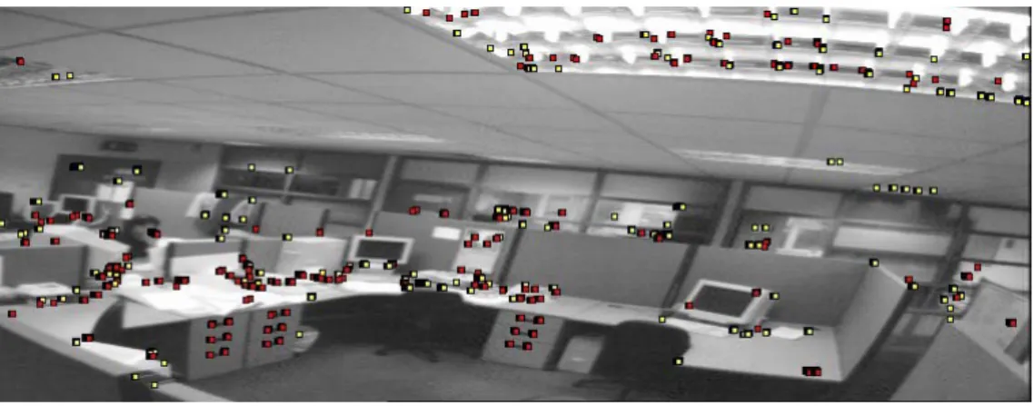
Figure 2.10 shows a corner detection using FAST, where positive and negative corners are distinguished as red and yellow.
Figure 2.10: FAST detection in a frame. From [RD05]
Table 2.1 presents the time taken to perform feature detection on a PAL field (768×288 pixels) on a test system, using FAST, SUSAN and Harris, detectors.
Table 2.1: Time taken to perform a feature detection with FAST, SUSAN and Harris. From [RD05].
Detector FAST SUSAN Harris Time (ms) 2,6 11,8 44
segment test. The arc with size 9 was proved to have more repeatability [RPD10]. More recently, FAST-ER algorithm was developed as a FAST successor. With a new heuristic for feature detection and using machine learning, it was demonstrated to represent significant improvements in repeatability, yielding a detector that is very fast and has a very high quality. The FAST-ER feature detector authors claim in [RPD10] (2010) it is able to fully process live PAL video using less than 5% of the available processing time. By comparison, most other detectors cannot even operate at frame rate (Harris detector 115%) [RPD10].
2.7
Outlier removal
Usually the corner matches are contaminated by outliers, i.e., wrong corner asso-ciations. Image noise, occlusions, blur, and changes in viewpoint and illumination are possible causes for outliers, that the mathematical model of the feature detector does not take into account [FS12]. Most feature matching techniques assume linear illumination changes, pure camera rotation and scaling, or affine distortions. Therefore, for an accurate estimation of the camera motion, it is crucial to remove the outliers. RANSAC is the most widely used method for outlier removal and is explained as follows.
2.7.1 RANSAC
2.7. OUTLIER REMOVAL 23
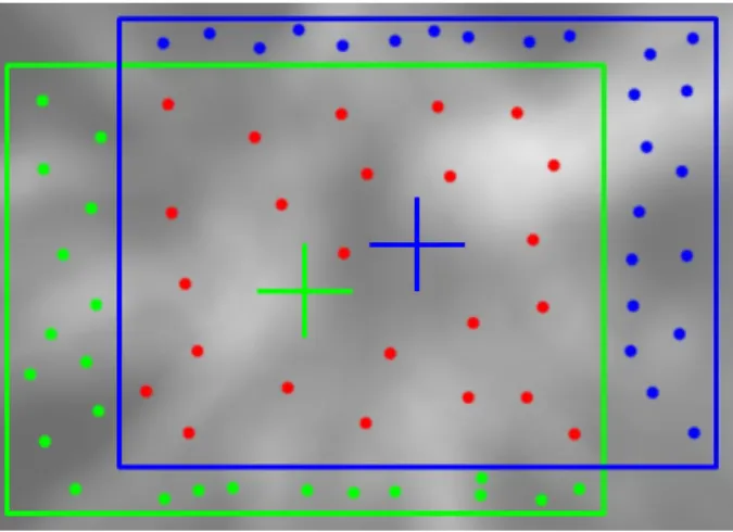
Figure 2.11 illustrates the estimation of a line that approximates the representing model of the inliers, contained on a set of data.
Figure 2.11: Estimated inliers of a data set contaminated with outliers.
For the stereo camera motion estimation, as used in VO, the estimated model is the relative motion between two camera positions, and the data points are the candidate features correspondences.
The RANSAC algorithm works as shown below. The input parameters of this algorithm are:
It - the number of iterations performed by the algorithm;
D - a set of data matches;
υ - the minimum number of data matches required to create the model;
d - maximum distance between a point and a model, to be considered an inlier.
The output parameter of this algorithm is:
Input :It,D,υ,d Output:C
while number of iterationsIt is not reached do
Select a sample of υ points fromD
Fit a model to these points
Compute the distance of all other points to this model
Count the number of points whose distance from the model is lower thand
(create the inlier set) Store these inliers
The solution of the problem is the set with the maximum number of inliers //
Estimate the model using all the inliers.
Algorithm 2.2: RANSAC.
The number of iterations necessary to guarantee that a correct solution is found can be computed as It= log(1−P)
log(1−(1−ǫ)s) whereǫis the percentage of outliers in the data points,
s is the number of data points from which the model can be instantiated, and P is the requested probability of success [FB81]. Usually Itis multiplied by a factor of 10 to make sure of the solution success. As illustrated, RANSAC is a probabilistic method and is non-deterministic considering it exhibits a different solution on different runs. Nevertheless, the solution tends to be stable when the number of iterations is increased.
2.8
Summary
SLAM aims to build a map of the environment and at the same time use the map to determine the location of the robot. Several sensors may be used for this purpose, such as: classical odometry, IMU, magnetic compasses, active beacons, visual odometry, LASER, among other. The sensors may be of type absolute or relative positioning. The absolute positioning sensors are more expensive and less flexible, considering it requires pre installed equipments in the environment. Therefore, relative positioning sensors are of major importance.
2.8. SUMMARY 25
which cause large position estimation errors. Magnetic compasses are efficient sensors when only the magnetic field of the Earth is present, otherwise it loses its functionality. Active beacons, as GPS, are very efficient and accurate, however it is very expensive due to its external equipments. IMU are very used nowadays, due to its low cost and con-sidering it has 6 DOF information. Visual Odometry is also very used and its number of supporters is growing nowadays. It is a cheap system that requires only a camera and is accurate when using robust algorithms.
Chapter 3
Visual Odometry and Mapping
This chapter illustrates the VO solution proposed in this dissertation. A perspective camera projection is used for the VO system. Picture frames are taken, with a certain tested resolution, for odometry analysis. The FAST corner detector is used to extract corners from these frames. FAST is detailed along with the differences between several FAST-n, varying n. For corner matching between frames, this work uses the common iterative method RANSAC. However, using RANSAC alone for corner matching would bring a high temporal complexity. Therefore, after detecting the corners in each frame, it is presented how corner signatures are created in order to allow the corner matching between frames. The algorithm FMBF is carefully detailed in order to prove the decrease of such complexity. Using the frames and the robot locations, a map is performed throughout the path. The camera calibration is performed using several pictures of a certain plane, with SI metrics written on it. The corner signature and picture frames simulators are used to validate the FMBF algorithm.
3.1
A Visual Odometry approach
3.1.1 Introduction
As mentioned previously, VO is the process of estimating the egomotion of a rigid body using only video input. The VO proposed approach consists on estimating the egomotion of a robot using a monocular scheme for video input. The robot is aimed to work on a
horizontal surface only, in an indoor environment, with a singular and perspective camera rigidly attached and pointed to the ceiling. The ceiling and the floor are both parallel planes, and are the means of interaction of the robot with the world. Considering the robot is wheeled and the camera has no proper motion, its image projection is also a plane, parallel to the ceiling.
Figure 3.1 presents a perspective view of the robot motion in one dimension. The ceiling is represented as a black line pattern, scanned by the camera (grey) with a field of view represented by the light green triangle. The body of the robot is shown as blue rectangle. The red arrow indicates the performed motion.
Figure 3.1: Perspective view of the robot, performing a one dimension movement.
While the robot moves, image features are extracted and matched throughout the picture frame sequence, enabling the estimation of the robot egomotion on the floor. There is no featuretriangulationand the full process is performed in 2D data. Hence, this system produces a 3 Degrees of Freedom (DOF) pose of the robot (x, y, yaw).
3.1. A VISUAL ODOMETRY APPROACH 29
Figure 3.2: Example of two successive picture frames taken to a certain ceiling. Top: geometric dispersions of both frames of the ceiling. Bottom: collected frame data.
3.1.1.1 Context
This VO approach uses a feature based type method. This means, features are extracted from each frame of the sequence, for egomotion estimation purpose [NNB04, CSS04]. Other authors use featureless motion estimation [MGD07]. Instead of detect-ing features, the harmonic 2D Fourier transform is applied in all the pixels from the two frames, in order to compute the relative motion. In feature based methods, features point out landmarks of the environment that are repeated over frames. When a robot movement is performed, there are landmarks that show up in the current frame and in the previous frame, in different locations. The pixel coordinates of the same landmark are known in both frames. Therefore, considering landmarks are physically static in the environment, through simple kinematics, the transformation matrix is calculated.
ceiling). Therefore, the distance between the planes is constant and it is assumed to be known in advance.
For feature correspondence in different frames, some authors use feature tracking method [Mor80, SLL01, MCM07], while others use feature matching [NNB04, Low03, How08, CECV14]. Feature tracking consists in detecting features in one frame and track them in the following frames, based on local search techniques. This method is recom-mended for small-scale environments, where motions between frames are short (it was used in the first VO researches). Feature matching consists on detecting and matching features independently based on similar metrics. This method is currently more employed, considering the increasing research on large-scale environments, and it is followed in this work.
After extracting corners from frames, the available metrics arecorner coordinates and corner symmetry. For the corner matching method to work, a set of algorithms is used, to obtain extra corner metrics. Those metrics are CS which are divided bydistance (Corner Distance Signature, CDS) and triangle (Corner Triangle Signature, CTS). Also, CTS is split in angle (Corner Triangle Angle Signature, CTAS) and distance (Corner Triangle Distance Signature, CTDS). CDS is a set of all the Euclidean distances (in pixels units) between the other corners of the frame and the corner respective to the signature. CTAS is a set of angle amplitudes of triangles, made by the respective corner and nearby chosen neighbours. CTDS is a set of pairs of distances made by the respective corner and the neighbours of the same triangle which performs CTAS. The corner symmetry describes if the respective corner is either much brighter or much darker than the arc of pixels from FAST detector. See section 3.1.3 and 3.1.4 for the explanation of these concepts.
3.1. A VISUAL ODOMETRY APPROACH 31
(NN) methodology [Bha10], FMBF finds the best fit of feature metrics for the corners that are extracted from consecutive frames. Section 3.1.5.2 describes this process in detail.
A block diagram in figure 3.3 represents the VO pipeline in this case study.
Figure 3.3: VO block diagram.
3.1.2 Picture frame capture
Picture frames are captured by a perspective camera model. Other authors with 3D approaches use omnidirectional camera models [GD00]. Such camera models have a field of view beyond 180 degrees, and could be useful for 3D mapping, considering the wide amount of the environment information at once.
Experimental results use a frame resolution of 320×240 pixel (i.e., 320 of width and 240 of height). Using this FAST approach (detailed in section 3.1.3) the experiments of this work prove that higher resolutions are not viable. Corners repeatability suffers a substantial decline and time consuming rises. For 3D approaches, where scale-variance is unavoidable, this problem is managed with FAST - Enhanced Repeatability (FAST-ER) [RPD10].
The ceiling observed by the camera is assumed to be a plane, with minimal roughness. There are no pre processing algorithms for image noise, camera shacking or blur treatment. The frames sampling rate changes with the algorithms time consumption. For different algorithms combinations and adjustments the sampling rate varies.
Figure 3.4: Perspective projection: scene plane (SI) and image plane (px) .
3.1.3 FAST feature detection
The FAST feature detector is a method that detects corner features in frames. There are several definitions of corners such as the result of geometric discontinuities, or small patches of texture. FAST computes a corner response and defines corners to be large local maxima of such response. This method requires frames with one colour channel, meaning grey scale intensity is considered on pixels. In order to test if a pixel is elected as a corner, a circle of 16 pixels (with a radius of 3) around a candidate cornerpis analysed. The circle
L∈ {1, ...,16} with locationsl∈Lconsists on pixels positioned relative to p, denoted by
p → l. A pixel p →l can be darker, brighter or similar to p, according to the difference between its intensity Ip→l and p intensity Ip, by a threshold t. These three states are presented as:
Sp→l=
d, Ip→l≤Ip−t (darker)
s, Ip−t < Ip→l≤Ip+t (similar)
b, Ip+t≤Ip→l (brighter)
(3.1)
The locations of an arc of n contiguous pixels, inside the circle, is denoted by A = {1, ..., n}, and each pixel location by a∈A. If the circle aroundp contains an arc p→A
with all pixels darker thenIp−tor brighter thenIp+t,pis considered a corner. Otherwise, no corner is considered. Let P be the set of all pixels in a frame. Three subsets of P are denoted as Pd,Ps andPb, where:
Pd={p∈P,∀a∈A:Sp→a=d}, (3.2)
3.1. A VISUAL ODOMETRY APPROACH 33
the set of pixels called positive corners, andPs are non corners.
FAST was originally made only for n = 12 arc size (FAST-12) [RD05]. Compared to other known corner detectors, such as DoG [Low04], SUSAN [SB97], Harris [HP88], Shi-Tomasi [ST94], FAST-12 is faster, but its repeatability is not higher. Years later, approaches of FAST-n [RPD10] were studied, with n∈ {9, ...,16}, and results prove that FAST-9 is the most efficient of FAST-n.
Figure 3.5 illustrates a 9 point segment test corner detection in an frame patch. The highlighted blue squares correspond to the 16 pixels of the circle, used in the corner detection. The pixel at p is the centre of a candidate corner. The arc is presented by the dashed green line that passes through 9 contiguous pixels.
Figure 3.5: FAST feature detection in a frame patch.
LetQbe a subset of locations ofL,Q={1,5,9,13}, shown in figure 3.6. To determine if p is a corner, the pixels p →Q are examined first. If Sp→1 and Sp→9 are both s, then
p can not be a corner. If p can still be a corner, pixels Sp→5 and Sp→13 are examined
similarly. This is a quick rejection that makes the algorithm faster.
For a certain n, the number of detected corners decreases with tincreasing. Hence, it is important to use an appropriatetto regulate the number of detected corners, depending on prior purposes. When a corner is found there are two implemented approaches. The faster one is to test each pixel of p → L in sequence, and stop when an arc p → A is found. The other approach is to keep testing the remaining p→L after p→A is found, for further analyses. With the complete information ofp∈P¯s corner circles in one frame, it is possible to control the number of detected corners on the next frame. This process is explained in section 3.1.7.1 in detail.
Figure 3.7 shows two successive frames (distinguished by different robot position) and the point corners at red (negative corners) and yellow (positive corners), extracted from FAST-9 with a thresholdt= 22.
3.1. A VISUAL ODOMETRY APPROACH 35
By decreasing the threshold tot= 18, figure 3.8 presents the increase of the extracted corners, using FAST-9.
Figure 3.8: Corner points extracted from FAST-9 witht= 18. Top: 222 corners. Bottom: 375 corners.
The different number of extracted corners between two successive frames occurs due to two possibilities. First, due to image noise or FAST detection imperfections (i.e., repeatability uncertainty). And second, due to the motion of the image projection, as figure 3.9 illustrates. The red corner points are extracted in both frames. The other corner points are extracted only in the respective colour frame.
![Figure 2.7: Illustration of the VO problem. From [FS11].](https://thumb-eu.123doks.com/thumbv2/123dok_br/16578065.738368/47.892.269.620.124.539/figure-illustration-vo-problem-fs.webp)