AN ADAPTIVE CONSTRAINT HANDLIG TECNIQUE FOR PARTICLE SWARM
IN CONSTRAINED OPTIMIZATION PROBLEMS
UMA TÉCNICA DE TRATAMENTO DE RESTRIÇÕES ADAPTATIVA PARA ENXAME DE PARTÍCULAS EM PROBLEMAS DE OTIMIZAÇÃO COM RESTRIÇÕES
Érica C.R. Carvalho1, José P.G. Carvalho2, Heder S. Bernardino3, Patrícia H. Hallak4, Afonso C.C. Lemonge4 1
Graduate Program of Computational Modeling, Federal University of Juiz de Fora, BRAZIL E-mail: ericacrcarvalho@gmail.com
2
Department of Applied and Computational Mechanics, Faculty of Engineering, Federal University of Juiz de Fora, BRAZIL E-mail: jose.carvalho@engenharia.ufjf.br
3
Department of Computer Science, Institute of Exact Sciences, Federal University of Juiz de Fora, BRAZIL E-mail: heder@ice.ufjf.br
4
Department of Applied and Computational Mechanics, Faculty of Engineering, Federal University of Juiz de Fora, BRAZIL E-mail: patricia.hallak@ufjf.edu.br, afonso.lemonge@ufjf.edu.br
RESUMO
Metaheurísticas inspiradas na natureza são largamente utilizadas para resolver problemas de otimização. No entanto, essas técnicas devem ser adaptadas ao resolver problemas de otimização com restrições, que são comuns em situações do mundo real. Aqui uma abordagem de penalização adaptativa (chamada Método de Penalização Adaptativa, APM) é combinada com uma técnica de Otimização por Enxame de Partículas (PSO) para resolver problemas de otimização com restrições. Esta abordagem é analisada utilizando um conjunto de problemas teste e 5 problemas de engenharia mecânica. Além disso, três variantes do APM são consideradas nos experimentos computacionais. A comparação dos resultados mostrou que o algoritmo proposto obteve um desempenho promissor na maioria dos problemas teste.
Palavras-chave: Otimização por Enxame de Partículas. Otimização com Restrições. Método de Penalização
Adaptativa.
ABSTRACT
Nature inspired meta-heuristics are largely used to solve optimization problems. However, these techniques should be adapted when solving constrained optimization problems, which are common in real world situations. Here an adaptive penalty approach (called Adaptive Penalty Method, APM) is combined with a particle swarm optimization (PSO) technique to solve constrained optimization problems. This approach is analyzed using a benchmark of test-problems and 5 mechanical engineering test-problems. Moreover, three variants of APM are considered in the computational experiments. Comparison results show that the proposed algorithm obtains a promising performance on the majority of the test problems.
1. INTRODUCTION
Optimization has been applied in many fields such as business, science, and engineering. Effective optimization techniques are important for improving the performance of applications and processes. A typical optimization problem has an objective function, equality/inequality constraints and upper/lower bounds on its decision variables. Most of the practical optimization problems are nonlinear and non-convex in either the objective and/or constraints, and so optimization of such problems requires a global optimization method (Zhang & Rangaiah, 2012).
In constrained optimization problems, one aims to minimize (or maximize) a function searching for the values of the design variables from a set of options (continuous, discrete, or mixed) which satisfy the set of constraints.
Evolutionary Algorithms (EAs) are stochastic optimization methods based on the principles of natural biological evolution (Han & Kim, 2002) and they are commonly applied to solve real-world optimization problems (Deb et al., 2002). An EA that has been obtained good results in several problems in the literature is Particle Swarm Optimization (PSO) (Eberhart & Kennedy, 1995), which is a population-based algorithm for optimization based on a simplified social model that is closely tied to swarming theory. The algorithm was developed based on the social behavior of some species of birds when searching for food (Eberhart & Kennedy, 1995). The PSO approach has a simple concept and this is easily implemented. Compared with other EAs, the main advantages of PSO are its robustness in controlling parameters and its high computational efficiency (Kennedy et al., 2001). A modified PSO called CRPSO and proposed by (Kar et al., 2012) is adopted here in order to avoid premature convergence. The CRPSO’s main feature is a new velocity expression and an operator called “craziness velocity".
Despite its robustness and global searching capacity, EAs were (originally) designed to be applied to unconstrained optimization problems. Thus, a constraint handling technique is necessary when this type of technique is applied to a constrained optimization problem.
The penalty function method has been the most popular constraint-handling technique in EAs due to its simple principle and easy implementation. The main difficulty of using a static penalty function lies in choosing appropriate values of penalty factors, which are problem-dependent (Kaveh & Talatahari, 2009). Many works in the literature discuss techniques to handle constraints with parameters chosen by the user, such as (Barbosa, 1999), (Koziel & Michalewicz, 1998), (Koziel & Michalewicz, 1999), (Orvosh & Davis, 1994) and (Runarsson & Yao, 2000). The presence of constraints significantly affects the performance of many optimization algorithms, including PSO.
APM (Adaptive Penalty Method), proposed by (Barbosa & Lemonge, 2002), is an adaptive approach to handle with constraints. APM does not require any type of user-defined penalty parameter and its penalty coefficients are calculated based on information obtained from the population, such as the average of objective function values and the level of violation of each constraint. Many works can be found in the literature where APM is used within EAs, for instance: Genetic Algorithms (Barbosa & Lemonge, 2002), Differential Evolution (Vargas et al., 2013)], and PSO (Carvalho et al., 2015). In addition to the original APM, several variants were proposed and analyzed by (Carvalho et al., 2015) when solving constrained structural optimization problems.
The performance of APM and some of its variants are analyzed here when coupled to the CRPSO algorithm solving constrained optimization problems. Several experiments are performed and the results are analyzed and compared to those obtained by other techniques from the literature.
The paper is organized as follows. In the next section the general constrained optimization problem is described. Section 3 presents a particle swarm algorithm. A brief discussion of techniques to
handle constrained optimization problems is presented in Section 4. Numerical experiments, with several test problems from the literature, are presented in Section 5. Finally, in Section 6, the conclusions and proposed future works are presented.
2. CONSTRAINED OPTIMIZATION PROBLEMS
A standard constrained optimization problem in can be defined as
(1) subject to
(2) (3) (4) where m is the number of constraints, n is the number of design variables, and and are the inequality and equality constraints, respectively. Usually, equality constraints are transformed into inequality ones as
(5)
where is the allowed tolerance of the equality constraints.
3. PARTICLE SWARM OPTIMIZATION
Particle Swarm Optimization (PSO) was proposed by (Eberhart & Kennedy, 1995). It is a population-based algorithm which has been inspired by the social behavior of animals, such as fish schooling, insects swarming and bird flocking. PSO was first applied to optimization problems with continuous variables (Parsopoulos & Vrahatis, 2002). The algorithm shows a faster convergence rate than other EAs for solving some optimization problems (Kennedy et al., 2001).
In PSO, each particle of the swarm represents a potential solution of the optimization problem. The particles fly through the search space and their positions are updated based on the best positions of individual particles in each iteration. The objective function is evaluated for each particle and the fitness values of particles are obtained in order to determine which position in the search space is the best one.
In each iteration, the swarm is updated using the following equations (Eberhart & Kennedy, 1995) (6)
where and represent the current velocity and the current position of the jth design variable of the
ith particle, respectively. is the best position of the ith particle (called pbest) and is the best
global position among all the particle in the swarm (called gbest); and are coefficients that control the influence of cognitive and social information, respectively, and and are two random values generated with uniform distribution between 0 and 1.
The basic PSO algorithm can be briefly described using the following steps: 1. Initialize randomly a particle swarm (positions) and velocities.
2. Initialize and .
3. Calculate the objective function value of each particle of the swarm.
4. Update and .
5. Update the position and velocity (Equations (6) and (7)). 6. Repeat the steps 3 to 5 until a stop condition is satisfied.
PSO has undergone many changes since its introduction in 1995. As researchers have learned about the technique, they have derived new versions, developed new applications, and published theoretical studies of the effects of the various parameters and aspects of the algorithm (Poli et al., 2007). An improved particle swarm optimization technique called Craziness based Particle Swarm Optimization (CRPSO), proposed by (Kar et al., 2012), is used here in order to get rid of the limitations of original PSO. The authors have modified the PSO by introducing an entirely new velocity expression associated with many random numbers and an operator called “craziness velocity”.
In CRPSO the velocity can be expressed as (Kar et al., 2012)
(8) where , , , and are random values uniformly taken from the interval [0,1), is a function defined as
(9) , the craziness velocity, is a user define parameter from the interval [ , ], and are defined, respectively, as
(10)
(11) and is a predefined probability of craziness. One can notice that while is a fixed value, varies every time the velocity is calculated.
4. AN ADAPTIVE PENALTY TECHNIQUE
The majority of engineering design problems involves constraints. Thus, appropriate methods for constraint handling are important. Evolutionary Algorithms can be seen as unconstrained search techniques since, in their original form, they do not incorporate any explicit mechanism to handle constraints. Because of this, several authors have proposed a variety of constraint-handling techniques explicitly designed for evolutionary algorithms (Coello, 2002), (Efren, 2009) and (Kicinger et al., 2005).
The most common approach in the EA community to handle constraints (particularly, inequality constraints) is to use penalty functions (Coello & Carlos, 1999). Several researchers have studied heuristics on the design of penalty functions. Probably the most well-known of these studies is the one conducted in (Richardson, 1989). The main idea is to transform a constrained optimization problem into an unconstrained one by adding a penalty function.
Penalty methods, although quite generally, require considerable domain knowledge and experimentation in each particular application in order to be effective. They can be also classified as static, dynamic and adaptive. Static penalty depends on the definition of an external factor to be added to or multiplied by the objective function. Dynamic penalty methods, in general, have penalty coefficients directly related to the number of generations, and the adaptive penalty considers the level of violation of the population by constraints during the evolutionary process. This paper does not attempt to cover the current literature on constraint handling and the reader is referred to survey papers or book chapters of e.g. (Barbosa et al., 2015), (Coello, 2002), (Mezura-Montes & Coello, 2011), (Michalewicz, 1995) and (Michalewicz & Schoenauer, 1996).
An adaptive penalty method (APM) was originally introduced by (Barbosa & Lemonge, 2002). The method uses information from the population, such as the average of the objective function and the level of violation of each constraint during the evolution. When using APM, the fitness function can be written as
(12) where
(13) and is the average of the objective function values in the current population.
The penalty parameter is defined at each generation as
(14) where is the violation of the jth constraint averaged over the current population.
Three variants of APM are analyzed here:
• Variant 3 (Barbosa & Lemonge, 2008): no penalty coefficient kj is allowed to have its value
• Variant 5 (Carvalho et al., 2015): is modified as
(15) where is the value of the objective function of the worst feasible individual (the average of the objective function values is used when no feasible individual exist).
• Variant 7 (Carvalho et al., 2015): , which originally represented the average of the violations of all individuals at each constraint, is defined here as the sum of the violation of all individuals which violate the j-th constraint divided by the number of individuals which violate this constraint. Also, , which represented the average of the objective function values, now denoted by , is the sum of the objective function values of all individuals in the current population divided by the number the infeasible individuals. Thus, is defined in Variant 7 as
. (16)
5. NUMERICAL EXPERIMENTS
In this section, the performance of the CRPSO when using APM or one of its variants is investigated on well-known and widely used test problems. The test-functions used in the computational experiments includes a set of 24 functions known as G-Suite (Liang et al., 2006) and 5 mechanical engineering optimization problems (Bernardino et al., 2007). Only feasible solutions were found in the 35 independents runs.
The parameters which were used for the CRPSO algorithm was a swarm size equal to 50, , , and . For Variant 3, the penalty parameter k is updated every 10 generations. It should be understood that discrete or integer design variables are considered as the nearest integer of the corresponding variable of the vector solution (particle). It points to either an index of a table of discrete values or an integer.
5.1. Performance analysis of experiments
The experiments are compared using the performance profiles proposed by (Dolan & Moré, 2002), an analytical resource for the visualization and interpretation of the results obtained in the numerical experiments.
Given a set of test problems , with , a set of algorithm with ,
and a performance metric (for instance, computational time), the performance ratio is defined as
Thus, the performance profile of the algorithm a is defined as
(18) where is the probability that the performance ratio of algorithm is within a factor of the best possible ratio. If the set P is a good representation of problems to be addressed, then algorithms with larger are to be preferred. The performance profiles have a number of useful properties (Barbosa et al., 2010) and (Dolan & Moré, 2002). Other studies using performance profiles in performance analysis of algorithms can be found in (Barbosa et al., 2010) and (Bernardino et al., 2011). 5.2. G-Suite
The first experiment is based in a popular suite of function presented in (Liang et al., 2006). The experiments were performed considering three levels of evaluations of the objective function: 5000, 50000 and 500000, commonly used in the literature for these experiments. The summary of the 24 test problems is given in Table 1 where n is the number of design variables, is the estimated rate between the feasible region and the search space, and ni and ne are the number of inequality and equality constraints, respectively.
Table 1: Summary of the 24 functions of G-Suite.
Problem N Type of (%) ni ne G01 13 quadratic 0.0111 9 0 G02 20 non-linear 99.9971 2 0 G03 10 polynomial 0.0000 0 1 G04 5 quadratic 52.1230 6 0 G05 4 cubic 0.0000 2 3 G06 2 cubic 0.0066 2 0 G07 10 quadratic 0.0003 8 0 G08 2 non-linear 0.8560 2 0 G09 7 polynomial 0.5121 4 0 G10 8 linear 0.0010 6 0 G11 2 quadratic 0.0000 0 1 G12 3 quadratic 4.7713 1 0 G13 5 non-linear 0.0000 0 3 G14 10 non-linear 0.0000 0 3 G15 3 quadratic 0.0000 0 2 G16 5 non-linear 0.0204 38 0 G17 6 non-linear 0.0000 0 4 G18 9 quadratic 0.0000 12 0 G19 15 non-linear 33.4761 5 0 G20 24 linear 0.0000 6 14 G21 7 linear 0.0000 1 5 G22 22 linear 0.0000 1 19 G23 9 linear 0.0000 2 4 G24 2 linear 79.6556 2 0
The average of the objective function values is used here as performance metric for the three levels of budget. Figure 1(a) shows the performance profiles in the range when 5000 objective function evaluations are allowed. In this case, Variant 5 presented the highest value of , indicating that this variant obtained the best performance in a larger number of problems. In Figure 1(b) it is possible to see that Variant 5 obtained the lowest value of such as assumes the largest value in that plot; this suggests that Variant 5 is also the most robust method between those analyzed here.
(a)
(b)
Figure 1: Performance profiles of the results obtained when solving G-Suite – 5000 objective function evaluations.
The performance profiles of the results obtained when using the 50000 objective function evaluations can be found in Figure 2(a) in which one can note that Variant 5 presented the best performance in the majority of the 24 test-problems. In Figure 2(b), one can seen that Variant 7 obtained the most robust solutions.
(a) (b)
Figure 2: Performance profiles of the results obtained when solving G-Suite – 50000 objective function evaluations. Finally, according to the performance profiles shown in Figure 3(a), Variant 3 presented the best performance in the majority of problems. On the other hand, Variant 7 presented more robustness, as one can see in Figure 3(b).
(a) (b)
Figure 3: Performance profiles of the results obtained when solving G-Suite – 500000 objective function evaluations. Besides the identification of the best performing technique in the majority of problems and the robustness one, performance profiles can be also used to indicate the method with the best performance in general; this can be made by means of the area under of the performance profiles curves (higher values are preferable). Table 2 present the normalized areas under the performance profiles curves for G-Suite, where nfe means the number of function evaluations. It can be observed that the best variant (in general)
for this set of 24 test-problems is Variant 7 which achieved 1 when using the 50000 and 500000 objective function evaluations, followed by the Variant 5 which achieved 1 when using 5000.
Table 2: Normalized areas under the performance profiles curves for G-Suite with 5000, 50000 and 500000 objective function evaluations.
Area
5000 nfe 50000 nfe 500000 nfe
APM 0.99992 0.89736 0.95185
Variant 3 0.94439 0.99995 0.90824
Variant 5 1 0.894736 0.92695
Variant 7 0.94437 1 1
5.3. Mechanical engineering problems
Five mechanical engineering problems are also used in this paper to evaluate the performance of the algorithm when using APM or one of its variants. Table 3 presents some details of each test problem where n is the number of design variables, ni and ne are the number of inequality and equality constraints, respectively and nfe is the number of function evaluations.
Table 3: Mechanical engineering problems.
Problem n Type of ni ne nfe
Welded Beam (WB) 4 quadratic 5 0 32000
Pressure Vessel (PV) 4 cubic 4 0 80000
Cantilever Beam (CB) 10 quadratic 11 0 35000
Speed Reducer (SR) 7 quadratic 11 0 36000
T./C. Spring (TCS) 3 non-linear 4 0 36000
In reference (Bernardino et al., 2007) it is possible obtain the description of the mechanical engineering problems used here. Figs. 4 to 8 illustrate each test-problem.
Figure 4: The Welded Beam.
Figure 5: The Pressure Vessel.
Figure 6: The Cantilever Beam.
Figure 7: The Speed Reducer.
Figure 8: The Tension/Compression Spring.
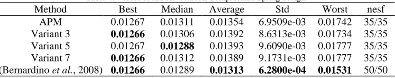
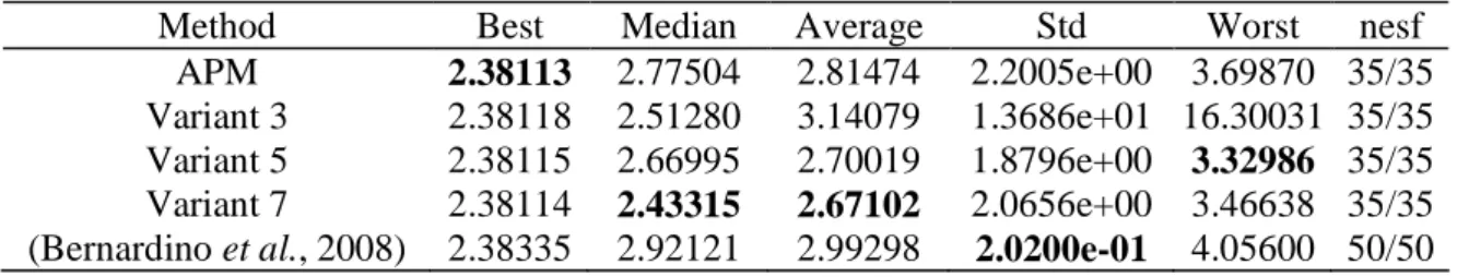
The results obtained for the mechanical engineering problems are presented in Tables 4, 6, 8, 10 and 12, where the best ones are displayed in boldface, and std means the standard deviation and nesf means the total number of independent runs in which feasible solutions were found. A hybridization of a Genetic Algorithm with an Artificial Immune System is proposed in (Bernardino et al., 2008) and its results are used here in the comparisons. It can be observed that in four of the five test-problems the APM or one of its variants achieved the best solution. Tables 5, 7, 9, 11 and 13 presents the design variables considering the best result for each problem for “This study” and reference (Bernardino et al., 2008).
Table 4: Values found for Tension/Compression Spring design.
Method Best Median Average Std Worst nesf
APM 0.01267 0.01311 0.01354 6.9509e-03 0.01742 35/35 Variant 3 0.01266 0.01306 0.01392 8.6313e-03 0.01734 35/35 Variant 5 0.01267 0.01288 0.01393 9.6090e-03 0.01777 35/35 Variant 7 0.01266 0.01312 0.01389 9.1731e-03 0.01777 35/35 (Bernardino et al., 2008) 0.01266 0.01289 0.01313 6.2800e-04 0.01531 50/50
Table 5: Comparison of results for Tension/Compression Spring design.
d D N Volume
This study 0.05406 0.41655 8.48436 0.01266
(Bernardino et al., 2008) 0.05143 0.35053 11.6612 0.01267
Table 6: Values found for Speed Reducer design.
Method Best Median Average std Worst nesf
APM 2996.3592 2996.3837 2998.8105 2.6529e+01 3007.4698 35/35 Variant 3 2996.3631 3005.7006 3003.6417 4.4687e+01 3016.7882 35/35 Variant 5 2996.3654 2996.3927 3002.1440 4.2637e+01 3016.7988 35/35 Variant 7 2996.3622 2996.3780 2999.6083 3.4911e+01 3016.7808 35/35 (Bernardino et al., 2008) 2996.3483 2996.3495 2996.3501 7.4500e-03 2996.3599 50/50
Table 7: Comparison of results for Speed Reducer design.
b m n l1 l2 d1 d2 Weight
This study 3.5000 0.7000 17 7.3009 8.2999 3.3502 5.2868 2996.3592 (Bernardino et al., 2008) 3.5000 0.7000 17 7.3000 7.8000 3.3502 5.2868 2996.3483
Table 8: Values found for Welded Beam design.
Method Best Median Average Std Worst nesf
APM 2.38113 2.77504 2.81474 2.2005e+00 3.69870 35/35 Variant 3 2.38118 2.51280 3.14079 1.3686e+01 16.30031 35/35 Variant 5 2.38115 2.66995 2.70019 1.8796e+00 3.32986 35/35 Variant 7 2.38114 2.43315 2.67102 2.0656e+00 3.46638 35/35 (Bernardino et al., 2008) 2.38335 2.92121 2.99298 2.0200e-01 4.05600 50/50
Table 9: Comparison of results for Welded Beam design.
h l t b Cost
This study 0.2444 6.2183 8.2912 0.2444 2.3811 (Bernardino et al., 2008) 0.2443 6.2186 8.2914 0.2443 2.3833
Table 10: Values found for Pressure Vessel design.
Method Best Median Average std Worst nesf
APM 6059.7143 6090.5263 6474.8760 3.1086e+03 7544.4925 35/35
Variant 3 6059.7143 6090.5263 6352.0563 2.5773e+03 7544.4925 35/35
Variant 5 6059.7143 6318.9481 6359.9781 2.2021e+03 7544.4925 35/35
Variant 7 6059.7143 6370.7797 6427.6676 2.6221e+03 7544.4925 35/35
(Bernardino et al., 2008) 6059.8546 6426.7100 6545.1260 1.2400e+02 7388.1600 50/50
Table 11: Comparison of results for Pressure Vessel design.
Ts Th R L Weight
This study 0.8750 0.4375 45.3367 140.2538 6059.7143 (Bernardino et al., 2008) 0.8125 0.4375 42.0973 176.6509 6059.8546
Table12: Values found for Cantilever beam design.
Method Best Median Average Std Worst nesf
APM 64965.071 67943.462 67901.329 1.6162e+04 75143.537 35/35 Variant 3 64584.132 68673.296 70516.546 4.2187e+04 106637.832 35/35 Variant 5 64578.229 67943.452 68240.218 1.6177e+04 73943.453 35/35
Variant 7 64578.271 68294.702 71817.816 1.0431e+05 173520.325 35/35 (Bernardino et al., 2008) 64834.700 74987.160 76004.240 6.9300e+03 102981.060 50/50
Table 13: Comparison of results for Cantilever beam design.
b1 h1 b2 h2 b3 h3 b4 h4 b5 h5 Volume
This study 4 60 3.1 55 2.6 50 2.204 44.091 1.749 34.995 64578.229 (Bernardino et al., 2008) 3 60 3.1 55 2.6 50 2.294 42.215 1.825 35.119 64834.700
The average of the results obtained by the variants is also used as performance metric in mechanical engineering problems. It can be observed in Figure 9(a), in the range , that APM is the variant with better performance in the majority of problems. Also, one can see that although Variant 5 obtained the best average value in none of the engineering optimization problems considered here (Figure 9(a)), this achieved the most robust results (Figure 9(b)).
(a) (b)
Figure 9: Performance profiles for mechanical engineering problems.
Table 9 present the normalized areas under the performance profiles curves for mechanical engineering problem. Variant 5 presented the high value for the normalized area under the performance profiles curves, followed by APM.
Table 9: Normalized areas under the performance profiles curves for mechanical engineering problems.
Method Area APM 0.96866 Variant 3 0.76332 Variant 5 1 Variant 7 0.94193
5.4. Summary of the results
One can observe that the standard version of APM and its variants performed well when applied to both, G-Suite and mechanical engineering problems. Variant 7 is the best performing technique (in general) when solving the G-Suite test-function (Table 2). Also, it is important to highlight that Variant 5 presented better results (in general) when this is compared to other APM variants and solving mechanical engineering problems (Table 9). Finally, one can notice that Variant 5 achieved the largest area under the performance profiles curves when only 5000 objective function evaluations are allowed.
6. CONCLUSION
A particle swarm optimization algorithm coupled with a method to handle with constraints called APM and three of its variants are tested in a well known set of constrained optimization problems in mathematical and mechanical engineering. A comparison with an alternative approach from the literature was performed and the PSO presented here provided competitive results in the computational experiments.
The results of the computational experiments for G-Suite demonstrate that Variant 7 and Variant 5 are more robust than Variants 3 and APM. Considering an analysis using the performance profiles, Variant 7 performed better than to the others variants for G-Suite. For the mechanical engineering problems, Variant 5 showed better results compared to the other variants.
For future works the proposed method is going to be applied to real world problems from engineering considering more complexity with respect to objective functions and constraints.
ACKNOWLEDGMENT
The authors thank CNPq (grants 306815/2011-7 and 305175/2013-0) and FAPEMIG (grants TEC PPM 528/11, TEC PPM 388/14 and APQ 00103-12) for their support.
7. REFERENCES
BARBOSA, H.J.C.: A coevolutionary genetic algorithm for constrained optimization. Evolutionary Computation, 1999. CEC 99. Proceedings of the 1999 Congress on, vol. 3. IEEE, 1999.
BARBOSA, H.J.C., BERNARDINO, H.S., BARRETO, A.M.S.: Using performance profiles to analyze
the results of the 2006 CEC constrained optimization competition. Evolutionary Computation (CEC),
2010 IEEE Congress on, pp. 1–8. IEEE, 2010.
BARBOSA, H.J.C., LEMONGE, A.C.C.: An adaptive penalty scheme in genetic algorithms for
BARBOSA, H.J.C., LEMONGE, A.C.C.: An adaptive penalty scheme in genetic algorithms for
constrained optimiazation problems. GECCO 2002: Proceedings o f the Genetic and Evolutionary
Computation Conference, pp. 287–294. Morgan Kaufmann Publishers, New York, 2002.
BARBOSA, H.J.C., LEMONGE, A.C.C.: An adaptive penalty method for genetic algorithms in
constrained optimization problems. Frontiers in Evolutionary Robotics 34, 2008.
BARBOSA, H.J.C., LEMONGE, A.C.C., BERNARDINO, H.S.: A critical review of adaptive penalty
techniques in evolutionary computation. Evolutionary Constrained Optimization, pp. 1–27. Springer,
2015.
BERNARDINO, H.S., BARBOSA, H.J., LEMONGE, A.C.: A hybrid genetic algorithm for constrained
optimization problems in mechanical engineering. 2007 IEEE Congress on Evolutionary Computation,
2007.
BERNARDINO, H.S., BARBOSA, H.J.C., FONSECA, L.G.: Surrogate-assisted clonal selection
algorithms for expensive optimization problems. Evolutionary Intelligence 4(2), 81–97, 2011.
BERNARDINO, H.S., BARBOSA, H.J.C., LEMONGE, A.C.C., FONSECA, L.G.: A new hybrid AIS-GA
for constrained optimization problems in mechanical engineering. Evolutionary Computation. CEC
(IEEE World Congress on Computational Intelligence). IEEE Congress on, pp. 1455–1462, 2008.
CARVALHO, E.C.R., BERNARDINO, H.S., HALLAK, P.H., LEMONGE, A.C.C.: An adaptive penalty
scheme to solve constrained structural optimization problems by a Craziness based Particle Swarm Optimization. Optimization and Engineering, 2015. To appear.
COELLO, C.A.C.: Theoretical and numerical constraint-handling techniques used with evolutionary
algorithms: a survey of the state of the art. Computer Methods in Applied Mechanics and
Engineering 191(11-12), 1245 – 1287, 2002.
COELLO, C.A.C., CARLOS, A.: A survey of constraint handling techniques used with evolutionary
algorithms. Lania-RI-99-04, Laboratorio Nacional de Informática Avanzada, 1999.
DEB, K., ANAND, A., JOSHI, D.: A computationally efficient evolutionary algorithm for real-parameter
optimization. Evolutionary computation 10(4), 371–395, 2002.
DOLAN, E.D., MORÉ, J.J.: Benchmarking optimization software with performance profiles. Mathematical Programming 91, 201–213, 2002.
EBERHART, R., KENNEDY, J.: A new optimizer using particle swarm theory. Micro Machine and Human Science. MHS’95., Proceedings of the Sixth International Symposium on, pp. 39–43. IEEE, 1995. EFREN, M.M.: Constraint-handling in evolutionary optimization. Pland: Springer, 2009.
HAN, K.H., KIM, J.H.: Quantum-inspired evolutionary algorithm for a class of combinatorial
KAR, R., MANDAL, D., MONDAL, S., GHOSHAL, S.P.: Craziness based particle swarm optimization
algorithm for fir band stop filter design. Swarm and Evolutionary Computation, 2012.
KAVEH, A., TALATAHARI, S.: Particle swarm optimizer, ant colony strategy and harmony search
scheme hybridized for optimization of truss structures. Computers & Structures 87(5), 267–283, 2009.
KENNEDY, J., KENNEDY, J.F., EBERHART, R.C., SHI, Y.: Swarm intelligence. Morgan Kaufmann Publishers, 2001.
KICINGER, R., ARCISZEWSKI, T., DE JONG, K.: Evolutionary computation and structural design: A
survey of the state-of-the-art. Computers & Structures 83(23), 1943–1978, 2005.
KOZIEL, S., MICHALEWICZ, Z.: A decoder-based evolutionary algorithm for constrained parameter
optimization problems. Parallel Problem Solving from Nature — PPSN V, pp.231–240. Springer, 1998.
KOZIEL, S., MICHALEWICZ, Z.: Evolutionary algorithms, homomorphous mappings, and constrained
parameter optimization. Evolutionary computation 7(1), 19–44, 1999.
LIANG, J., RUNARSSON, T.P., MEZURA-MONTES, E., CLERC, M., SUGANTHAN, P., COELLO, C.C., DEB, K.: Problem definitions and evaluation criteria for the CEC 2006 special session on
constrained real-parameter optimization. Journal of Applied Mechanics 41, 8, 2006.
MEZURA-MONTES, E., COELLO, C.A.C.: Constraint-handling in nature -inspired numerical
optimization: Past, present and future. Swarm and Evolutionary Computation 1(4), 173–194, 2011.
MICHLEWICZ, Z.: A survey of constraint handling techniques in evolutionary computation methods. Proc. of the 4th Annual Conference on Evolutionary Programming, pp. 135–155. MIT Press, 1995.
MICHLEWICZ, Z., SCHOENAUER, M.: Evolutionary algorithms for constrained parameter
optimization problems. Evolutionary computation 4(1), 1–32, 1996.
ORVOSH, D., DAVIS, L.: Using a genetic algorithm to optimize problems with feasibility constraints. Evolutionary Computation, 1994. IEEE World Congress on Computational Intelligence., Proceedings of the First IEEE Conference on, pp. 548–553. IEEE, 1994.
PARSOPOULOS, K.E., VRAHATIS, M.N.: Recent approaches to global optimization problems through
particle swarm optimization. Natural computing 1(2-3), 235–306, 2002.
POLI, R., KENNEDY, J., BLACKWELL, T.: Particle swarm optimization. Swarm intelligence 1(1), 33– 57, 2007.
RICHARDSON, J.T., PALMER, M.R., LIEPINS, G.E., HILLIARD, M.: Some guidelines for genetic
algorithms with penalty functions. Proceedings of the third international conference on Genetic
algorithms, pp. 191–197. Morgan Kaufmann Publishers Inc., 1989.
RUNARSSON, T.P., YAO, X.: Stochastic ranking for constrained evolutionary optimization. Evolutionary Computation, IEEE Transactions on 4(3), 284–294, 2000.
VARGAS, D.E., LEMONGE, A.C., BARBOSA, H.J., BERNARDINO, H.S.: Differential evolution with
the adaptive penalty method for constrained multiobjective optimization. Evolutionary Computation
(CEC), 2013 IEEE Congress on, pp. 1342–1349, 2013.
ZHANG, H., RANGAIAH, G.: An efficient constraint handling method with integrated differential
evolution for numerical and engineering optimization. Computers & Chemical Engineering 37, 74–88,