António Afonso & Rui Carvalho
Revenue Forecast Errors in the
European Union
WP02/2014/DE/UECE
_________________________________________________________ De pa rtme nt o f Ec o no mic s
W
ORKINGP
APERSRevenue Forecast Errors in the European Union
António Afonso
$, Rui Carvalho
#October 2013
Abstract
In this paper we assess the determinants of revenue forecast errors for the EU-15 between 1999 and 2012, based on the forecasts published bi-annually by the European Commission. Our results show that personal income rate changes increase the revenue forecast errors: for forecasts made in t for t, increases in the corporate tax rate implies a
decrease in the revenue forecast errors, in t+1 and t+2. Moreover, an increase in GDP
forecast errors decreases revenue errors, whereas an increase in the inflation error will increase revenue errors. GDP errors, minority governments, election year and corporate tax rate changes can be associated with optimistic revenue forecasts. On the other hand, yield, inflation errors and VAT tax rate changes are associated with more prudent forecast behaviour.
Keywords: macro forecasts, revenue forecast errors, EU
JEL: C23, H20, H68
$ ISEG/ULisbon – University of Lisbon, Department of Economics; UECE – Research Unit on
Complexity and Economics, R. Miguel Lupi 20, 1249-078 Lisbon, Portugal, email: [email protected]. UECE is supported by Fundacão para a Ciência e a Tecnologia (Portuguese Foundation for Science and Technology) through the project PEst-OE/EGE/UI0436/2011. European Central Bank, Directorate General Economics, Kaiserstraße 29, D-60311 Frankfurt am Main, Germany. The opinions expressed herein are those of the authors and do not necessarily reflect those of the ECB or the Eurosystem.
1. Introduction
In recent years there was significant uncertainty regarding macroeconomic forecasts made not only by international institutions but also by central governments. This fact was visible notably when the Organisation for Economic Co-operation and Development (OECD) fiscal outlook, for a wide range of countries, showed that the tax revenue was much lower than officially predicted at the beginning of the financial crisis in 2008 (Buettner & Kauder, 2010; Golosov & King, 2002). This fact was also recently brought to light in the Report of Central Administration Budget Execution for 2012 elaborated by the Portuguese Court of Auditors (2013), where the recent evolution of the value added tax (VAT) raised doubts about the sustainability of forecasts1.
In fact, making precise revenue forecasts is not an easy job. To predict government revenues, one needs to take into account a wide set of variables from the most basic macroeconomic variables, as gross domestic product (GDP) or inflation, to fiscal policy, tax structures, and, perhaps the most difficult one to model, people’s behaviour towards uncertainty.
One of the reasons why the forecasts have a key role in the economy is the expectations generated by them. Macroeconomic data may take a few years until it become definitive, so in the meanwhile, forecasts are the best existing values and the ones taken into account by investors when it comes to evaluate the capability of a country to face its responsibilities. Moreover, as identified by Esteves and Braz (2013) access to reliable information on the economic situation is fundamental for policy makers since the results of their actions depend on the quality of the available information.
In this paper, we study the variables mentioned by the literature as more likely to influence the performance of revenue forecast. For that purpose, a panel data set was constructed based on the biannual reports made by the European Commission (EC), from 2000 spring up to 2013 spring, for the European Union (EU) 15 countries: Austria (AT), Belgium (BE), Germany (DE), Denmark (DK), Spain (ES), Finland (FI), France (FR), Greece (GR), Ireland (IE), Italy (IT), Luxembourg (LU), Netherlands (NL), Portugal (PT), Sweden (SW) and United Kingdom (UK). In addition, a seemingly unrelated regression (SUR) analysis for each country will be performed in order to identify possible cross-country differences.
Our results show that personal income rate changes increase the revenue forecast errors: for forecasts made in t for t, increases in the corporate tax rate implies a decrease
in the revenue forecast errors, in t+1 and t+2. Moreover, an increase in GDP forecast
errors decreases revenue errors, whereas an increase in the inflation error will increase revenue errors. GDP errors, minority governments, election year and corporate tax rate changes can be associated with optimistic revenue forecasts. On the other hand, yield, inflation errors and VAT tax rate changes are associated with more prudent forecast behaviour.
The paper is organised as follows. Section 2 reviews the literature about forecast errors, mainly on the revenue side. Section 3 presents the empirical analysis. Finally, section 4 is the conclusion.
2. Literature review
In the study of Golosov and King (2002) the main focus concerning forecast errors were the ones around the forecast of the GDP growth rate. However, and recognizing that having accurate revenue data is fundamental in order to elaborate a good budget, countries and authorities have made efforts to obtain reliable numbers for expected revenues (Buettner & Kauder, 2010), and so the discussion around this issue has increased. Nevertheless, the majority of the existing literature about revenue forecasting concerns the USA (Buettner & Kauder, 2010; Golosov & King, 2002).
On the other hand, it was not the first time that revenue forecast errors was used as an attempt to explain a crisis. According to Auerbach (1995) economists were trying to explain the ongoing fiscal crisis on the USA by looking at tax changes in the 1980s and early 1990s. Based on the Office of Management and Budget (OMB) annual budget forecasts, the author explained the deviations of revenue using an unusual approach, by trying to explain the determinants of technical errors. The results supported the idea that overly optimistic revenue forecasts from the 1980s were partially caused by unforeseen reactions from taxpayers.
Cimadomo (2011), in his literature survey about real-time data and fiscal policy analysis, identified that frequent and sizeable revisions of fiscal data, as well as large deviations of fiscal outcomes from the initial forecasts, are factors that endanger the
EU’s surveillance mechanism. Model uncertainty or unexpected shocks, are pointed out
as the main reasons for fiscal outcomes deviations’ from government plans. Upcoming political elections are also mentioned as possibly inducing over-optimism in fiscal projections.
Buettner and Kauder (2010) studied the performance of revenue forecasts for 12 OECD countries. They argued that cross-country differences in revenue forecasting performance were mainly caused by the uncertainty about macroeconomic variables, corporate and personal income tax structures, the elapsed time between the forecast and the observation of the variables, and the independence of forecasts from possible government manipulation.
Golosov and King (2002), assessed one year-ahead forecasts of tax revenues in the International Monetary Fund (IMF) programs for a group of low income countries. The authors mentioned that the latest studies (at the time) did not found any link between forecasting errors and political factors. They also report that underestimates of next
year’s fiscal deficit would be much more expensive than overestimating by the same
value. As a consequence, it was suggested that since the fiscal deficit underestimation is more expensive then overestimation, the deviation should occur on the cheaper side. In the context of an IMF program, major changes to the tax system may take place and those changes may introduce additional uncertainty to the forecasts of tax revenues.
Using data from the annual Stability and Convergence Programs, for the EU-15 countries, Hagen (2010) studied the deviations between projected and actual outcomes for several variables, namely GDP growth, general government budget balance, revenues and expenditures relative to GDP. The author found both problems in the forecasting performance of the EU country governments and bias and inefficiency regarding the projections. As a consequence, Hagen (2010) says that these facts lead us to wonder about the capability of governments to carry out accurate forecasts, as well as their availability to reveal all the detained information.
induce over-optimistic forecasts. On the contrary, commitment, mix forms of fiscal governance and numerical expenditure rules are frequently linked to higher carefulness when it comes to forecasts.
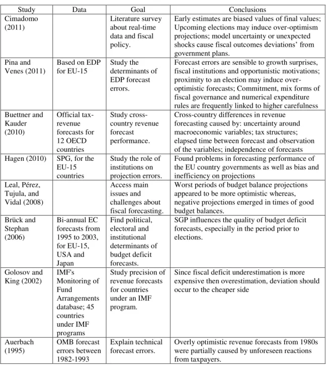
Table I – Summary of literature
Study Data Goal Conclusions
Cimadomo (2011)
Literature survey about real-time data and fiscal policy.
Early estimates are biased values of final values; Upcoming elections may induce over-optimism projections; model uncertainty or unexpected
shocks cause fiscal outcomes deviations’ from
government plans. Pina and
Venes (2011)
Based on EDP for EU-15
Study the determinants of EDP forecast errors.
Forecast errors are sensible to growth surprises, fiscal institutions and opportunistic motivations; proximity to an election may induce over-optimistic forecasts; Commitment, mix forms of fiscal governance and numerical expenditure rules are frequently linked to higher carefulness Buettner and Kauder (2010) Official tax-revenue forecasts for 12 OECD countries Study cross-country revenue forecast performance.
Cross-country differences in revenue forecasting caused by: uncertainty around macroeconomic variables; tax structures; elapsed time between forecast and observation of the variables; independence of forecasts Hagen (2010) SPG, for the
EU-15 countries
Study the role of institutions on projection errors.
Found problems in forecasting performance of the EU country governments as well as bias and inefficiency on projections
Leal, Pérez, Tujula, and Vidal (2008) Access main issues and challenges about fiscal forecasting.
Worst periods of budget balance projections appeared to be more optimistic whereas, negative projections emerged in times of good budget balances. Brück and Stephan (2006) Bi-annual EC forecasts from 1995 to 2003, for EU-15, USA and Japan Find political, electoral and institutional determinants of budget deficit forecasts.
SGP influences the quality of budget deficit forecasts, especially in the period prior to elections. Golosov and King (2002) IMF's Monitoring of Fund Arrangements database; 45 countries under IMF programs
Study precision of revenue forecasts for countries under an IMF program.
Since fiscal deficit underestimation is more expensive then overestimation, deviation should occur to the cheaper side
Auerbach
(1995) OMB forecast errors between 1982-1993
Explain technical
forecast errors. Overly optimistic revenue forecasts from 1980s were partially caused by unforeseen reactions from taxpayers.
A literature survey by Leal, Pérez, Tujula, and Vidal (2008) regarding the main issues and challenges about fiscal forecasting, finds that in the worst periods budget balance projections appeared to be more optimistic whereas, negative projections emerged in times of better budget balances.
Therefore, the literature has already identified possible outcomes for having inaccurate forecasts. However, the results seem to vary across time and country. Table I summarizes some of the abovementioned main findings.
3. Empirical analysis
3.1 Methodology
Since we want to address forecast errors, it is essential to enlighten this concept. Following the literature (Afonso & Silva, 2012, Hagen, 2010, Pina & Venes, 2011) we consider a forecast error the difference between the variable outturn and the variable forecast, where i stands for the country and t for the corresponding forecast period,
(1) .
Thus, positive values for errors are the result of a better than projected performance, while a negative value represents an overly optimistic forecast. Note that, it is considered as outturn, for period t, the first available estimate published by the EC on
t+1 (the spring forecast).2
3.2 European Commission Forecasts
In this sub-section we analyse the revenue forecasts of the EC for the EU-15 countries. Hence, our main data sources are based on the bi-annual reports published by the EC, between 1999 spring and 2013 spring. The data were collected for years t, t+1
and t+2 for GDP growth in volume, for the private consumption price deflator, general
government total revenue as percentage of GDP, plus the first available estimates for these same variables. Subsequently, and using the methodology explained in (1), our main variables were constructed, namely the GDP error, inflation error and revenue as a percentage of GDP.
From the Annual Macroeconomic database of the EC (AMECO), we used the general government consolidated gross debt (DEBT), the general government balance
(BAL), and the gap between actual and potential GDP (GAP). The 10-year bond yield is taken from Eurostat’s European Monetary Union (EMU) convergence criterion series. Standard & Poor's 500 volatility index (VIX) was taken from yahoo finance and used later as an instrumental variable.
Using a political database from Armingeon et al. (2012)3, a set of dummies was used in order to control for political influences, specifically, coalition governments’
(Coalition), legislative elections in the present year (Election year) and minority governments composed by one party (Minority Gov).
The EC has carried out a survey across the member states, in order to assess what kind of numerical fiscal rules are used – budget balance, revenue, expense, among others. According to the EC, the purpose of these rules is to increase fiscal discipline and serve as an instrument for policy coordination between member states, furthermore reducing the uncertainty on fiscal policy. Thus, the variable fiscal rule index (FRI) is also used in order to check whether such rules have any influence on the revenue predictions.
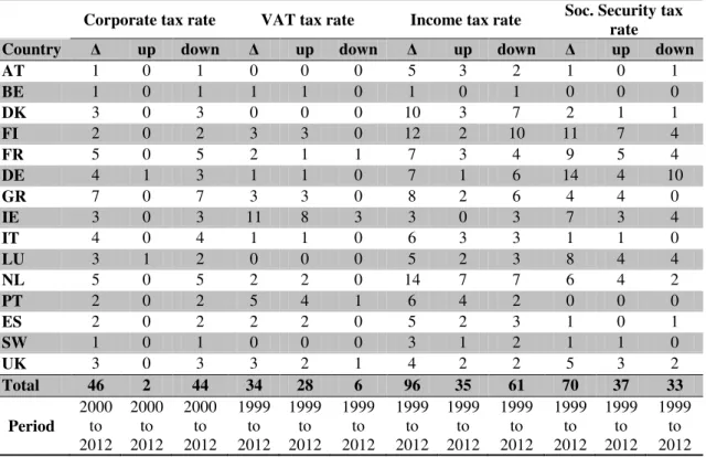
Finally, in order to capture the uncertainty resulting from the changes in the tax rates and in the law, a series of dummies was used. Generally, they assume the value 1 when a change in the tax rate relative to previous year occurs and 0 in the opposite case. Therefore, we can account for changes in VAT rates, changes in the personal income tax rate, changes in the corporate tax rate and changes in social security tax rates. Apart from these variables, there are also dummies for each of the taxes that indicate whether if the observed changed was due to an increase or a decrease of the rate, which allows ascertaining more precisely the impact of each change. All these variables were based on the OECD Tax Database, except for the VAT.4
Table II shows that changes to personal income rates are the most frequent ones, whereas changes to VAT are the less frequent. For instance, there are only two increases of corporate tax rates in the sample, contrasting with the high number of increases in income tax rates.
Overall, the main reason for choosing all the above mentioned variables is because they are the most used in the literature, not only to study revenue deviations but also in
3 Data for 2011 was kindly provided by the authors, while the 2012 calculations were based on
www.parlagov.org/ and on the same methodology.
related studies about other macroeconomic variables, like expenditure, budget deficits, GDP.
Table II - Dummy distribution, by tax type, country and direction of change
Corporate tax rate VAT tax rate Income tax rate Soc. Security tax rate
Country Δ up down Δ up down Δ up down Δ up down
AT 1 0 1 0 0 0 5 3 2 1 0 1
BE 1 0 1 1 1 0 1 0 1 0 0 0
DK 3 0 3 0 0 0 10 3 7 2 1 1
FI 2 0 2 3 3 0 12 2 10 11 7 4
FR 5 0 5 2 1 1 7 3 4 9 5 4
DE 4 1 3 1 1 0 7 1 6 14 4 10
GR 7 0 7 3 3 0 8 2 6 4 4 0
IE 3 0 3 11 8 3 3 0 3 7 3 4
IT 4 0 4 1 1 0 6 3 3 1 1 0
LU 3 1 2 0 0 0 5 2 3 8 4 4
NL 5 0 5 2 2 0 14 7 7 6 4 2
PT 2 0 2 5 4 1 6 4 2 0 0 0
ES 2 0 2 2 2 0 5 2 3 1 0 1
SW 1 0 1 0 0 0 3 1 2 1 1 0
UK 3 0 3 3 2 1 4 2 2 5 3 2
Total 46 2 44 34 28 6 96 35 61 70 37 33
Period 2000 to 2012 2000 to 2012 2000 to 2012 1999 to 2012 1999 to 2012 1999 to 2012 1999 to 2012 1999 to 2012 1999 to 2012 1999 to 2012 1999 to 2012 1999 to 2012 Source: OECD Tax database and authors' calculations. – number of changes.
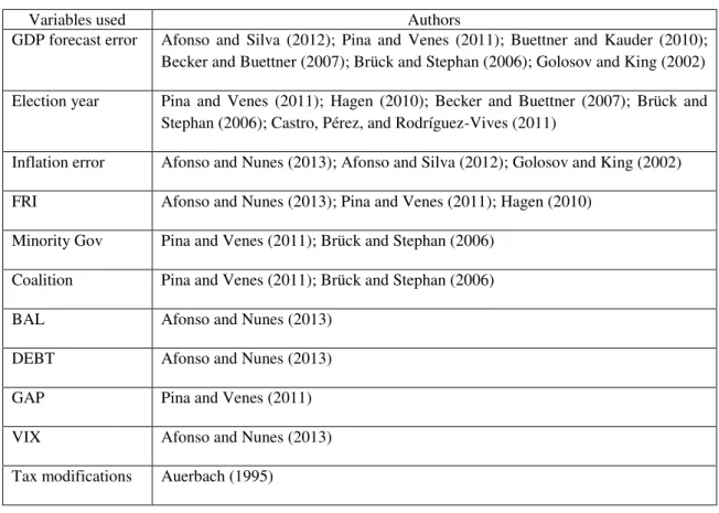
Table III illustrates some of the papers that have used the above described variables, or similar ones, in studies related with forecast errors. Thus, using this set of variables, which can be classified as economic, political and technical, we assess their explanatory power for each of the types of errors associated with the literature for errors in revenue forecasts.
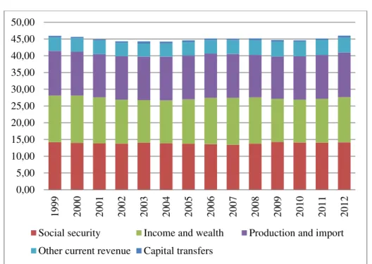
In addition, it is important to stress which components contribute for the general
government’s total revenue. The EC follows the European System of Accounts 95 (ESA95) nomenclature5. Hence, total revenue is the sum of taxes on production and imports (D.2), other subsidies on production (D.39), property income (D.4), current taxes on income and wealth (D.5), social contributions (D.61), other current transfers (D.7) and capital transfer (D.9).
Table III – Summary of main variables in previous studies
Variables used Authors
GDP forecast error Afonso and Silva (2012); Pina and Venes (2011); Buettner and Kauder (2010); Becker and Buettner (2007); Brück and Stephan (2006); Golosov and King (2002)
Election year Pina and Venes (2011); Hagen (2010); Becker and Buettner (2007); Brück and Stephan (2006); Castro, Pérez, and Rodríguez-Vives (2011)
Inflation error Afonso and Nunes (2013); Afonso and Silva (2012); Golosov and King (2002)
FRI Afonso and Nunes (2013); Pina and Venes (2011); Hagen (2010)
Minority Gov Pina and Venes (2011); Brück and Stephan (2006)
Coalition Pina and Venes (2011); Brück and Stephan (2006)
BAL Afonso and Nunes (2013)
DEBT Afonso and Nunes (2013)
GAP Pina and Venes (2011)
VIX Afonso and Nunes (2013)
Tax modifications Auerbach (1995)
Figure 1 - Annual total revenue for EU-15, per category (% of GDP)
Source: AMECO.
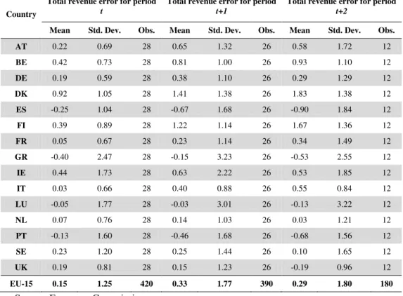
Table IV shows the descriptive statistics for our dependent variables, the revenue error as a percentage of GDP, for all EU-15 countries. Observing the mean value for the EU-15 we conclude that for all periods, the realized revenue has been, on average, higher than forecasts, suggesting the existence of ex-ante prudent behaviour. In practice, revenue outturn was, on average, 0.15 percentage points higher than forecasted for t,
0.33 percentage points higher for t+1 and 0.29 percentage points higher for t+2.
0,00 5,00 10,00 15,00 20,00 25,00 30,00 35,00 40,00 45,00 50,00
19
99
20
00
20
01
20
02
20
03
20
04
20
05
20
06
20
07
20
08
20
09
20
10
20
11
20
12
Table IV – Descriptive statistics for revenue errors (% of GDP)
Country
Total revenue error for period
t
Total revenue error for period
t+1
Total revenue error for period
t+2
Mean Std. Dev. Obs. Mean Std. Dev. Obs. Mean Std. Dev. Obs.
AT 0.22 0.69 28 0.65 1.32 26 0.58 1.72 12
BE 0.42 0.73 28 0.81 1.00 26 0.93 1.10 12
DE 0.19 0.59 28 0.38 1.10 26 0.29 1.29 12
DK 0.92 1.05 28 1.41 1.38 26 1.83 1.38 12
ES -0.25 1.04 28 -0.67 1.68 26 -0.90 1.84 12
FI 0.39 0.89 28 1.22 1.14 26 1.67 1.36 12
FR 0.05 0.67 28 0.23 1.14 26 0.34 1.49 12
GR -0.40 2.47 28 -0.15 3.23 26 -0.53 2.55 12
IE 0.44 1.73 28 0.63 2.22 26 0.53 1.85 12
IT 0.03 0.66 28 0.40 0.88 26 0.55 0.84 12
LU -0.05 1.77 28 -0.03 3.01 26 -0.13 3.22 12
NL 0.07 0.76 28 0.14 1.03 26 0.03 1.21 12
PT -0.13 1.60 28 -0.46 1.68 26 -0.68 1.56 12
SE 0.23 1.20 28 0.25 1.44 26 0.10 1.65 12
UK 0.19 0.81 28 0.15 1.23 26 -0.19 0.96 12
EU-15 0.15 1.25 420 0.33 1.77 390 0.29 1.80 180
Source: European Commission.
However, this is not true for all EU-15 countries. Greece, Portugal, Spain and Luxembourg exhibit negative mean forecast errors for all the periods, in other words, forecast revenues were optimistic. In addition, for Portugal and Spain, the longer is the forecasted period, the higher the negative error, on average. This behaviour is not shared by Luxembourg and Greece, where t+1 forecasts emerge as the most accurate ones, on
average. Besides those countries, only the United Kingdom reveals a negative forecast mean for t+2.
Nevertheless, if we make an average per country for the three periods, the United Kingdom emerges as the country with most accurate forecasts, followed by Luxembourg and the Netherlands. On the opposite side, Denmark, Finland and Belgium are the ones with most inaccurate forecasts, even though they all under predict revenue (see table A.1, on appendix).
3.3 Panel Estimation
unbalanced panel data set, with the earlier described variables, from 1999 to 2012, for the EU-15 (Austria, Belgium, Germany, Denmark, Spain, Finland, France, Greece, Ireland, Italy, Luxembourg, Netherlands, Portugal, Sweden and United Kingdom).
The starting point for the analysis of each year can be represented by the following equation:
(2) = + + ( ) +
( ) + ( ) + + +
+ + +
+ + +
where i represents the year-semester of the forecast and t represents the year for which
the forecast refers.
For each one of the forecasting horizons’ a baseline model is used, allowing us to have comparisons between those years. We have done additional estimations, depending on which of the tax change dummies is significant. Regarding robustness, in order to make sure that our baseline was the most adequate, we also tried different lags and removed variables that decreased the number of observations.
Following (Afonso & Nunes, 2013), due to possible correlation between DEBT and BAL, it was decided not to include both variables at the same time in our model. Nonetheless, both equations were tested, and the results were very similar. For this reason and since the r-square for the BAL specification was slightly higher, in the remaining work we have used this variable.
All the estimations were made using country fixed effects, creating a dummy that will account for all the omitted variables for that country. Moreover, all the equations use white diagonal covariance matrix, which consent residual heteroscedasticity (Afonso & Nunes, 2013).
Suspecting the possible existence of endogeneity between the and the , we performed the Wu-Hausman endogeneity test. In order to run this test, one should start by regressing the suspecting problematic variable on its instruments – in this case the ones used were the VIX(-1) and the (-1),
0.10 we can reject endogeneity. In this case, we did not found evidence of endogeneity evidence in any regression.
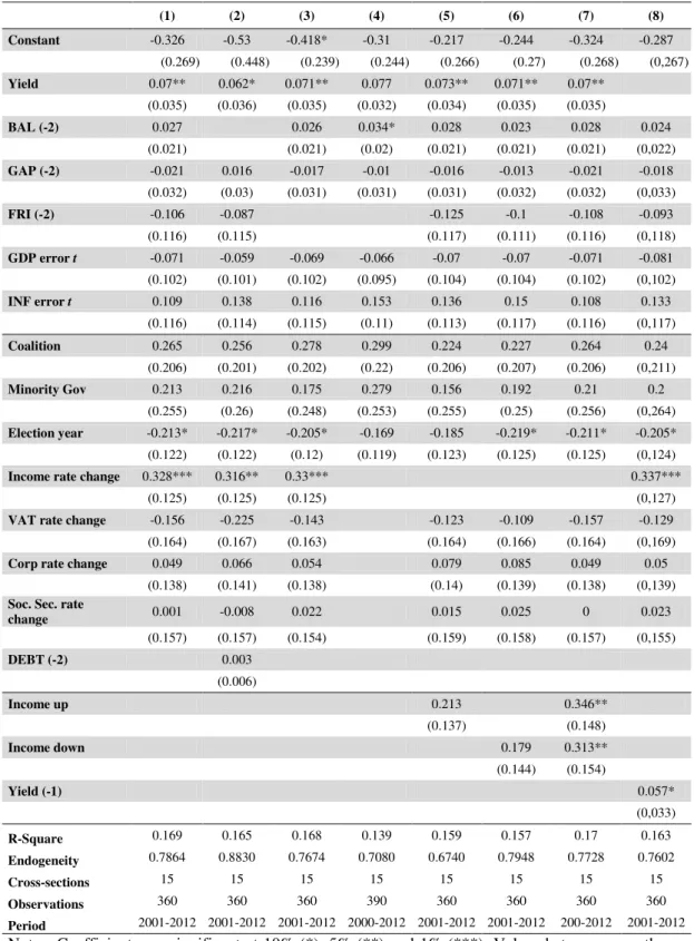
Table V, reports the results using forecasts made in t for t. Three variables emerge
as the most significant ones. Income rate changes of 1 p.p. lead to an increase, on average, of 0.328 p.p. of revenue errors. Also, a 1 p.p. change in the 10-year yield results in a 0.07revenue error increase, on average. On the other hand, legislative elections taking place in year t have the opposite effect. The existence of an election in
year t will result in a decrease of revenue error of 0.212 p.p., on average.
In addition, and knowing that income rate changes lead to higher errors, we checked whether these errors were caused by an increase or a decrease in personal income tax rates, in columns (5), (6) and (7). However, none of the effects is significant when tested individually, column (7) tests for the combined effect. The effects are significant at 5 % and both have positive coefficients. Therefore, if the personal income rate changes, the revenue error will be higher, for forecasts made in t for t.
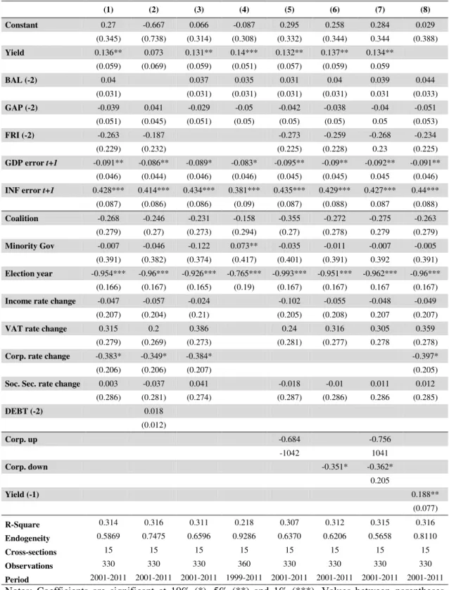
Regarding the estimations reported in Table VI for revenue error estimations made in year t for t+1, we observe an increase on the number of significant variables, when
comparing with the results from Table V. As before, the yield is significant and with a similar impact as well as the lagged yield. The election year is again important but now with higher significance. On average, the existence of an election in t will result in a
decrease of the revenue error of 0.934 p.p. in the GDP error on t+1 and in the INF error
on t+1, and these effects are now significant, which broadly goes into the direction
pointed by literature.
An increase of 1 p.p. of the GDP error for the following year will result on average in -0.9 p.p. on the revenue error whereas the INF error for t+1 will increase the revenue
error in 0,424 p.p. Changes to the corporate tax rate are significant in all equations. Overall, changes to corporate tax rate will result in a decrease of the revenue error of
0.378 on average. By controlling for “up” and “down” corporate tax rate dummies’, we conclude that decreases in the corporate tax rate in year t, decrease the revenue forecast
Table V – Total revenue error estimation, for year t
(1) (2) (3) (4) (5) (6) (7) (8) Constant -0.326 -0.53 -0.418* -0.31 -0.217 -0.244 -0.324 -0.287
(0.269) (0.448) (0.239) (0.244) (0.266) (0.27) (0.268) (0,267)
Yield 0.07** 0.062* 0.071** 0.077 0.073** 0.071** 0.07**
(0.035) (0.036) (0.035) (0.032) (0.034) (0.035) (0.035)
BAL (-2) 0.027 0.026 0.034* 0.028 0.023 0.028 0.024
(0.021) (0.021) (0.02) (0.021) (0.021) (0.021) (0,022)
GAP (-2) -0.021 0.016 -0.017 -0.01 -0.016 -0.013 -0.021 -0.018
(0.032) (0.03) (0.031) (0.031) (0.031) (0.032) (0.032) (0,033)
FRI (-2) -0.106 -0.087 -0.125 -0.1 -0.108 -0.093
(0.116) (0.115) (0.117) (0.111) (0.116) (0,118)
GDP error t -0.071 -0.059 -0.069 -0.066 -0.07 -0.07 -0.071 -0.081 (0.102) (0.101) (0.102) (0.095) (0.104) (0.104) (0.102) (0,102)
INF error t 0.109 0.138 0.116 0.153 0.136 0.15 0.108 0.133 (0.116) (0.114) (0.115) (0.11) (0.113) (0.117) (0.116) (0,117)
Coalition 0.265 0.256 0.278 0.299 0.224 0.227 0.264 0.24 (0.206) (0.201) (0.202) (0.22) (0.206) (0.207) (0.206) (0,211)
Minority Gov 0.213 0.216 0.175 0.279 0.156 0.192 0.21 0.2 (0.255) (0.26) (0.248) (0.253) (0.255) (0.25) (0.256) (0,264)
Election year -0.213* -0.217* -0.205* -0.169 -0.185 -0.219* -0.211* -0.205*
(0.122) (0.122) (0.12) (0.119) (0.123) (0.125) (0.125) (0,124)
Income rate change 0.328*** 0.316** 0.33*** 0.337***
(0.125) (0.125) (0.125) (0,127)
VAT rate change -0.156 -0.225 -0.143 -0.123 -0.109 -0.157 -0.129
(0.164) (0.167) (0.163) (0.164) (0.166) (0.164) (0,169)
Corp rate change 0.049 0.066 0.054 0.079 0.085 0.049 0.05
(0.138) (0.141) (0.138) (0.14) (0.139) (0.138) (0,139)
Soc. Sec. rate
change 0.001 -0.008 0.022 0.015 0.025 0 0.023
(0.157) (0.157) (0.154) (0.159) (0.158) (0.157) (0,155)
DEBT (-2) 0.003 (0.006)
Income up 0.213 0.346**
(0.137) (0.148)
Income down 0.179 0.313** (0.144) (0.154)
Yield (-1) 0.057*
(0,033)
R-Square 0.169 0.165 0.168 0.139 0.159 0.157 0.17 0.163 Endogeneity 0.7864 0.8830 0.7674 0.7080 0.6740 0.7948 0.7728 0.7602 Cross-sections 15 15 15 15 15 15 15 15 Observations 360 360 360 390 360 360 360 360 Period 2001-2012 2001-2012 2001-2012 2000-2012 2001-2012 2001-2012 200-2012 2001-2012
Notes: Coefficients are significant at 10% (*), 5% (**) and 1% (***). Values between parentheses stand for the standard errors. Endogeneity represents the p-value taken from Wu-Hausman endogeneity test for GDP error t. Cross-sections is the number of included countries. Period
Table VI - Total revenue error estimation, for year t+1
(1) (2) (3) (4) (5) (6) (7) (8) Constant 0.27 -0.667 0.066 -0.087 0.295 0.258 0.284 0.029
(0.345) (0.738) (0.314) (0.308) (0.332) (0.344) 0.344 (0.388)
Yield 0.136** 0.073 0.131** 0.14*** 0.132** 0.137** 0.134** (0.059) (0.069) (0.059) (0.051) (0.057) (0.059) 0.059
BAL (-2) 0.04 0.037 0.035 0.031 0.04 0.039 0.044 (0.031) (0.031) (0.031) (0.031) (0.031) 0.031 (0.033)
GAP (-2) -0.039 0.041 -0.029 -0.05 -0.042 -0.038 -0.04 -0.051
(0.051) (0.045) (0.051) (0.05) (0.05) (0.05) 0.05 (0.053)
FRI (-2) -0.263 -0.187 -0.273 -0.259 -0.268 -0.234
(0.229) (0.232) (0.225) (0.228) 0.23 (0.225)
GDP error t+1 -0.091** -0.086** -0.089* -0.083* -0.095** -0.09** -0.092** -0.091**
(0.046) (0.044) (0.046) (0.046) (0.045) (0.045) 0.045 (0.046)
INF error t+1 0.428*** 0.414*** 0.434*** 0.381*** 0.435*** 0.429*** 0.427*** 0.44***
(0.087) (0.086) (0.086) (0.09) (0.087) (0.088) 0.087 (0.088)
Coalition -0.268 -0.246 -0.231 -0.158 -0.355 -0.272 -0.275 -0.263
(0.279) (0.27) (0.273) (0.294) (0.27) (0.278) 0.279 (0.279)
Minority Gov -0.007 -0.046 -0.122 0.073** -0.035 -0.011 -0.007 -0.005
(0.391) (0.382) (0.374) (0.417) (0.401) (0.391) 0.392 (0.391)
Election year -0.954*** -0.96*** -0.926*** -0.765*** -0.993*** -0.951*** -0.962*** -0.96*** (0.166) (0.167) (0.165) (0.19) (0.167) (0.167) 0.167 (0.167)
Income rate change -0.047 -0.057 -0.024 -0.102 -0.055 -0.048 -0.049 (0.207) (0.204) (0.21) (0.205) (0.208) 0.207 (0.207)
VAT rate change 0.315 0.2 0.386 0.24 0.316 0.305 0.359
(0.279) (0.269) (0.273) (0.281) (0.277) 0.278 (0.278)
Corp. rate change -0.383* -0.349* -0.384* -0.397*
(0.206) (0.206) (0.207) (0.205)
Soc. Sec. rate change 0.003 -0.037 0.041 -0.018 -0.01 0.011 0.012
(0.286) (0.281) (0.274) (0.287) (0.286) 0.286 (0.285)
DEBT (-2) 0.018
(0.012)
Corp. up -0.684 -0.756
-1042 1041
Corp. down -0.351* -0.362*
0.205
Yield (-1) 0.188** (0.077)
R-Square 0.314 0.316 0.311 0.218 0.307 0.312 0.315 0.316 Endogeneity 0.5869 0.7475 0.6596 0.9286 0.6370 0.6206 0.5658 0.8110 Cross-sections 15 15 15 15 15 15 15 15 Observations 330 330 330 360 330 330 330 330 Period 2001-2011 2001-2011 2001-2011 1999-2011 2001-2011 2001-2011 2001-2011 2001-2011
Notes: Coefficients are significant at 10% (*), 5% (**) and 1% (***). Values between parentheses stand for the standard errors. Endogeneity represents the p-value taken from Wu-Hausman endogeneity test for GDP error t+1. Cross-section is the number of included countries. Period represents covered
years.
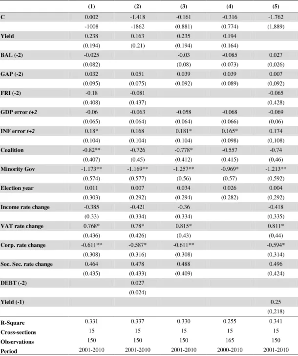
Table VII - Total revenue error estimation, for year t+2 (excluding up and down dummies)
(1) (2) (3) (4) (5)
C 0.002 -1.418 -0.161 -0.316 -1.762
-1008 -1862 (0.881) (0.774) (1,889)
Yield 0.238 0.163 0.235 0.194
(0.194) (0.21) (0.194) (0.164)
BAL (-2) -0.025 -0.03 -0.085 0.027
(0.082) (0.08) (0.073) (0,026)
GAP (-2) 0.032 0.051 0.039 0.039 0.007
(0.095) (0.075) (0.092) (0.089) (0,092)
FRI (-2) -0.18 -0.081 -0.065
(0.408) (0.437) (0,428)
GDP error t+2 -0.06 -0.063 -0.058 -0.068 -0.069
(0.065) (0.064) (0.064) (0.066) (0,06)
INF error t+2 0.18* 0.168 0.181* 0.165* 0.174
(0.104) (0.104) (0.104) (0.098) (0,108)
Coalition -0.82** -0.726 -0.778* -0.557 -0.74
(0.407) (0.45) (0.412) (0.415) (0,46)
Minority Gov -1.173** -1.169** -1.257** -0.969* -1.213**
(0.574) (0.577) (0.56) (0.57) (0,592)
Election year 0.011 0.007 0.034 0.026 0.004
(0.303) (0.292) (0.294) (0.282) (0,292)
Income rate change -0.385 -0.421 -0.36 -0.418
(0.33) (0.334) (0.334) (0,335)
VAT rate change 0.768* 0.78* 0.815* 0.811*
(0.436) (0.426) (0.43) (0,44)
Corp. rate change -0.611** -0.587* -0.611** -0.594*
(0.308) (0.316) (0.308) (0,314)
Soc. Sec. rate change 0.464 0.478 0.488 0.496
(0.435) (0.433) (0.409) (0,424)
DEBT (-2) 0.027 (0.024)
Yield (-1) 0.25 (0,218)
R-Square 0.331 0.337 0.330 0.255 0.341 Cross-sections 15 15 15 15 15 Observations 150 150 150 165 150 Period 2001-2010 2001-2010 2001-2010 2000-2010 2001-2010
Notes: Coefficients are significant at 10% (*), 5% (**) and 1% (***). Values between parentheses stand for the standard errors. Endogeneity represents the p-value taken from Wu-Hausman endogeneity test for GDP error t+2. Cross-section is the number of included countries. Period
represents covered years.
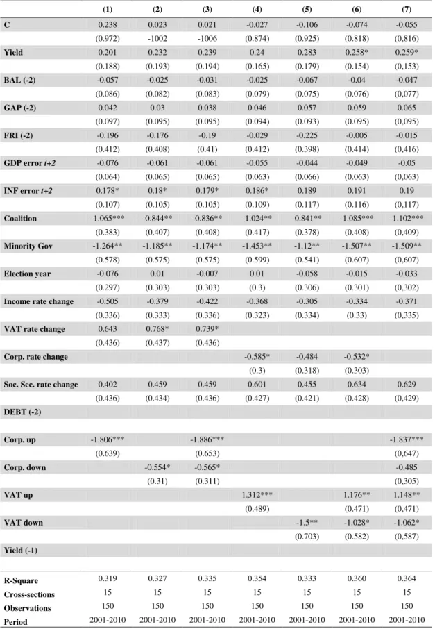
In Table VII we present the results for the 2-years ahead revenue forecasts. In this case the yield is not significant anymore but the inflation errors, for t+2, remain
average. In this horizon, two tax changes are statistically significant: the VAT rate changes contribute to an increase of revenue errors while corporate tax rate changes drive up revenue error decreases’.
Table VIII allows a better overview of the effects of those rate changes. Estimated individually, all the effects are significant but equation (7) discloses that decreases on the corporate rate are no longer significant. On the other hand, increases on the corporate tax rate reduce the revenue error for t+2 by 1.837 p.p. This is particularly surprising because there are only two changes on this variable, one for Germany (2003) and another for Luxembourg (2011). From (7) we can also observe that only increases to the VAT tax rate implies an increase of revenue errors.
Therefore, one can conclude that besides GDP and inflation errors, the other economic variables do not seem to be directly connected to the revenue forecast errors contrasting with institutional and political variables that emerged as the most significant determinants explaining the errors.
Another interesting relation is the one between tax changes and their weight in total revenue. Social security contributions are the ones that contribute the most for total revenue in the EU-15. However, none of the estimated equations showed statistical significance regarding social security rate changes even though there were approximately 70 changes in the social security contribution rates, across countries.
Comparing the results from Tables V, VI and VII with the ones in Table IV –
concerning the descriptive statistic of revenue errors – we observe that t+1 had the
higher mean error and it is for the t+1 estimations that one can find more statistically
significant variables. On the contrary, the mean error for t and t+2 was lower, and we
also found less significant variables in those estimations.
For robustness purposes, we used instrumental variables for all t and t+1 equations.
Table VIII - Total revenue error estimation, for year t+2 (including up and down dummies)
(1) (2) (3) (4) (5) (6) (7)
C 0.238 0.023 0.021 -0.027 -0.106 -0.074 -0.055
(0.972) -1002 -1006 (0.874) (0.925) (0.818) (0,816)
Yield 0.201 0.232 0.239 0.24 0.283 0.258* 0.259* (0.188) (0.193) (0.194) (0.165) (0.179) (0.154) (0,153)
BAL (-2) -0.057 -0.025 -0.031 -0.025 -0.067 -0.04 -0.047
(0.086) (0.082) (0.083) (0.079) (0.075) (0.076) (0,077)
GAP (-2) 0.042 0.03 0.038 0.046 0.057 0.059 0.065
(0.097) (0.095) (0.095) (0.094) (0.093) (0.095) (0,095)
FRI (-2) -0.196 -0.176 -0.19 -0.029 -0.225 -0.005 -0.015
(0.412) (0.408) (0.41) (0.412) (0.398) (0.414) (0,416)
GDP error t+2 -0.076 -0.061 -0.061 -0.055 -0.044 -0.049 -0.05
(0.064) (0.065) (0.065) (0.063) (0.066) (0.063) (0,063)
INF error t+2 0.178* 0.18* 0.179* 0.186* 0.189 0.191 0.19
(0.107) (0.105) (0.105) (0.109) (0.117) (0.116) (0,117)
Coalition -1.065*** -0.844** -0.836** -1.024** -0.841** -1.085*** -1.102***
(0.383) (0.407) (0.408) (0.417) (0.378) (0.408) (0,409)
Minority Gov -1.264** -1.185** -1.174** -1.453** -1.12** -1.507** -1.509** (0.578) (0.575) (0.575) (0.599) (0.541) (0.607) (0,607)
Election year -0.076 0.01 -0.007 0.01 -0.058 -0.015 -0.033 (0.297) (0.303) (0.303) (0.3) (0.306) (0.301) (0,302)
Income rate change -0.505 -0.379 -0.422 -0.368 -0.305 -0.334 -0.371 (0.336) (0.333) (0.336) (0.323) (0.334) (0.33) (0,335)
VAT rate change 0.643 0.768* 0.739* (0.436) (0.437) (0.436)
Corp. rate change -0.585* -0.484 -0.532* (0.3) (0.318) (0.303)
Soc. Sec. rate change 0.402 0.459 0.459 0.601 0.455 0.634 0.629 (0.436) (0.434) (0.436) (0.427) (0.421) (0.428) (0,429)
DEBT (-2)
Corp. up -1.806*** -1.886*** -1.837***
(0.639) (0.653) (0,647)
Corp. down -0.554* -0.565* -0.485
(0.31) (0.311) (0,305)
VAT up 1.312*** 1.176** 1.148**
(0.489) (0.471) (0,471)
VAT down -1.5** -1.028* -1.062*
(0.703) (0.582) (0,587)
Yield (-1)
R-Square 0.319 0.327 0.335 0.354 0.333 0.360 0.364 Cross-sections 15 15 15 15 15 15 15 Observations 150 150 150 150 150 150 150 Period 2001-2010 2001-2010 2001-2010 2001-2010 2001-2010 2001-2010 2001-2010
Notes: Coefficients are significant at 10% (*), 5% (**) and 1% (***). Values between parentheses stand for the standard errors. Endogeneity represents the p-value taken from Wu-Hausman endogeneity test for GDP error t+2. Cross-section is the number of included countries. Period
3.4 SUR system
In order to have country specific results, we have run a SUR analysis for year t and
t+1. Because of the reduced number of observations it was not possible to estimate the
model for year t+2. Another reason for using this approach is that regardless the
previous results, is that there are cross-country differences that cannot be unveiled with simple panel data. Not all countries are influenced by the same variables and with the same intensity.
The SUR model works by running an estimation for each country but at the same time allows for contemporary correlation between the residuals of all equations which is more efficient than performing an OLS for each country. For our case, the following equation was used:
(3) = + + ( ) +
( ) + +
where i denotes the country and t the year forecasted.
The reason for using a reduced form of the baseline model is that the SUR does not support the use of dummy variables. Moreover, it is also not possible to use the FRI since its values are close to a constant over time. In addition, another SUR was performed excluding lagged output gap and can be found in the Appendix (A.4 and A.5).
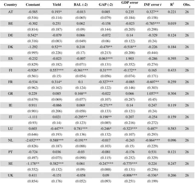
Observing Table IX, the results are slightly different from the previous equations. It may be noted that there are more significant negative coefficients, than negative. The output GAP is the variable that is more frequently statistically significant. For Denmark, France, Ireland, Luxembourg and Sweden, as GAP increases, the revenue error seems to be reduced, whereas for Spain, Finland and Italy the tendency is to increase, while Portugal does not have a single significant variable. The inflation errors affect roughly half of the countries. Another result is that, significant GDP errors only contribute to the reduction of the revenue errors.
Table IX - SUR system per country, for total revenue error as a percentage of
GDP, for year t
Country Constant Yield BAL (-2) GAP (-2) GDP error
t INF error t R
2 Obs.
AT -0.585 0.193* -0.013 0.085 0.235 0.327** 0.221 26
(0.516) (0.114) (0.065) (0.079) (0.184) (0.158)
BE -0.302 0.251 0.062 -0.158 -0.023 -0.785*** 0.019 26
(0.814) (0.187) (0.09) (0.144) (0.205) (0.298)
DE 0.542* -0.079 0.066 -0.072 0.14 -0.329 0.124 26
(0.316) (0.083) (0.049) (0.06) (0.122) (0.24)
DK -1.292 0.52** 0.218 -0.479** -0.518** -0.226 0.184 26
(0.995) (0.226) (0.17) (0.213) (0.208) (0.444)
ES -0.232 -0.023 -0.007 0.063*** 1.903 -0.286 0.395 26
(0.829) (0.182) (0.071) (0.131) (0.352) (0.274)
FI -0.926* 0.557*** -0.361*** 0.31*** -0.172** 0.165 0.433 26 (0.561) (0.15) (0.054) (0.056) (0.074) (0.171)
FR -0.534 0.314* 0.1 -0.327*** -0.085 -0.607** 0.259 26
(0.962) (0.162) (0.124) (0.122) (0.146) (0.303)
GR 0.229 0.085 0.168** -0.022 0.066 1.057** 0.304 26
(0.679) (0.069) (0.077) (0.107) (0.287) (0.45)
IE 0.911 -0.066 0.069 -0.271** 0.14 0.247 0.119 26
(0.901) (0.206) (0.058) (0.133) (0.121) (0.24)
IT -1.111 0.021 -0.295** 0.198** 0.207 -0.254 0.159 26
(0.93) (0.14) (0.123) (0.085) (0.216) (0.272)
LU 0.603 -0.447** 0.781*** -0.246* -0.323*** 0.487* 0.583 26
(0.646) (0.193) (0.136) (0.132) (0.107) (0.293)
NL -2.652*** 0.588*** -0.191** -0.017 -0.243 -0.864*** 0.096 26 (0.826) (0.187) (0.088) (0.103) (0.15) (0.229)
PT -0.724 0.036 -0.03 -0.081 -0.176 0.531 0.121 26
(0.497) (0.075) (0.098) (0.115) (0.252) (0.329)
SE -1.178** 0.382*** 0.061 -0.247*** -0.775*** 0.224 0.247 26 (0.552) (0.132) (0.09) (0.088) (0.131) (0.256)
UK 0.411 -0.151 -0.058 0.09 -0.806*** -0.336* 0.266 26
(0.854) (0.176) (0.052) (0.093) (0.251) (0.199)
Note: Coefficients are significant at 10% (*), 5% (**) and 1% (***). Values between parentheses stand for the standard errors. Obs. represent the number of observations for the specific country
As expected, Table X, regarding the forecasts for t+1, has more significant values
then the previous one. Also, contrary to Table IX, there are now more positive significant coefficients pushing up the revenue error.
The Netherlands is now the country with more statistically significant variables followed by Luxembourg, Spain and Germany. Significant inflation errors’ coefficients only display positive signs, resulting in an increase of the revenue error when the inflation errors increase as well. For instance, for t+1, Portugal has now yield, BAL and
Generally, one can conclude that the variables affect countries in different ways. Despite that, it is not possible to conclude which coefficients have higher impact on revenue errors, if the positive or the negative ones.
Table X - SUR system per country, for total revenue error as a percentage of GDP, for year t+1
Country Constant Yield BAL (-2) GAP (-2) GDP error
t+1
INF error
t+1 R
2 Obs.
AT -1.292 0.161 -0.404*** 0.486*** -0.076 0.824*** 0.448 26
-1.095 (0.257) (0.089) (0.125) (0.105) (0.184)
BE -2.928** 0.951*** -0.083 -0.216 0.261* -0.164 0.056 26
-1.449 (0.364) (0.118) (0.194) (0.149) (0.191)
DE 3.082*** -0.69*** 0.152** -0.335*** -0.216** 0.07 0.494 26
(0.699) (0.175) (0.065) (0.08) (0.084) (0.188)
DK 0.435 0.207 -0.031 -0.138 -0.403*** 0.4 0.208 26
-1.318 (0.302) (0.186) (0.24) (0.125) (0.322)
ES -3.997*** 1.094*** 0.275*** -0.376** 1.069*** -0.23 0.562 26 -1.162 (0.277) (0.093) (0.175) (0.137) (0.168)
FI -1.22 0.71*** -0.283*** 0.26*** -0.013 0.054 0.434 26
(0.786) (0.21) (0.079) (0.076) (0.051) (0.151)
FR 2.069 0.057 0.335 -0.674** 0.158 -0.113 0.468 26
-2.507 (0.373) (0.287) (0.266) (0.131) (0.224)
GR -1.066 0.389*** 0.307** 0.007 -0.116 1.041*** 0.331 26
-1.133 (0.132) (0.143) (0.248) (0.167) (0.283)
IE 3.169*** -0.397** 0.035 -0.39*** 0.33*** -0.108 0.739 26
(0.782) (0.179) (0.05) (0.114) (0.059) (0.094)
IT -1.922* 0.149 -0.471*** 0.245*** 0.029 0.008 0.205 26
(0.938) (0.163) (0.121) (0.086) (0.082) (0.138)
LU -0.102 -0.623** 0.659*** 0.056 -0.776*** 1.644*** 0.796 26
(0.894) (0.252) (0.158) (0.152) (0.085) (0.183)
NL -2.943*** 0.76*** -0.189** 0.396*** 0.243*** 0.291*** 0.642 26
(0.894) (0.215) (0.095) (0.097) (0.081) (0.112)
PT -0.69 -0.731*** -0.803*** 0.342*** 0.076 -0.044 0.499 26
(0.425) (0.084) (0.089) (0.105) (0.104) (0.107)
SE -1.71* 0.443** -0.022 -0.038 -0.137 -0.075 0.241 26
(0.892) (0.204) (0.156) (0.119) (0.087) (0.381)
UK 0.082 -0.096 -0.102 0.055 0.126 0.248 0.164 26
-1.454 (0.297) (0.095) (0.139) (0.141) (0.207)
4. Conclusions
Having in mind that forecasting is a complex task surrounded by huge uncertainty, we have tried find the possible determinants of revenue forecasting errors. Therefore, we used the EC bi-annual forecasts that were made for the period 1999-2012.
Our results allow confirm what the literature had previously documented, that is, the existence of different sources for revenue errors, namely, economic, political and technical. A particular important result is that tax rate changes do affect revenue errors and that different tax changes affect differently the revenue errors. If, on the one hand, personal income rate changes increase the revenue error, for forecasts made in t for t,
increases in the corporate tax rate implies a decrease in the revenue forecast errors, in
t+1 and t+2. We also confirmed that an increase in GDP forecast errors decreases
revenue errors, whereas an increase in the inflation error will increase revenue errors. GDP errors, minority governments, election year and corporate tax rate changes can be associated with optimistic revenue forecasts. On the other hand, yield, inflation errors and VAT tax rate changes are associated with more prudent forecast behaviour.
References
Afonso, A., & Nunes, A. S. (2013). Economic forecasts and sovereign yields: Department of Economics at the School of Economics and Management (ISEG), Technical University of Lisbon.
Afonso, A., & Silva, J. (2012). The Fiscal Forecasting Track Record of the European Commission and Portugal: Department of Economics at the School of Economics and Management (ISEG), Technical University of Lisbon.
Armingeon, K., Weisstanner, D., Engler, S., Potolidis, P., & Gerber, M. (2012).
Comparative Political Data Set I 1960-2010. Bern: Institute of Political Science,
University of Bern.
Auerbach, A. J. (1995). Tax Projections and the Budget: Lessons from the 1980's.
American Economic Review, 85(2), 165-169.
Auerbach, A. J. (1999). On the Performance and Use of Government Revenue Forecasts: Berkeley Olin Program in Law & Economics.
Becker, I., & Buettner, T. (2007). Are German Tax-Revenue Forecasts Flawed? Ifo
Breuer, C. (2013). On the Uncertainty of Tax Revenue Projections: A Forecast Error
Decomposition for New German Data. Leibnutz Institute for Economic Research at
the Universiy of Munich. Munich.
Brück, T., & Stephan, A. (2006). Do Eurozone Countries Cheat with their Budget Deficit Forecasts? Kyklos, 59(1), 3-15.
Buettner, T., & Kauder, B. (2010). Revenue Forecasting Practices: Differences across Countries and Consequences for Forecasting Performance. Fiscal Studies, 31(3),
313-340.
Castro, F. d., Pérez, J. J., & Rodríguez-Vives, M. (2011). Fiscal data revisions in Europe: European Central Bank.
Cimadomo, J. (2011). Real-time data and fiscal policy analysis: a survey of the literature: European Central Bank.
Esteves, P. S., & Braz, C. R. (2013). Previsão de curto prazo das receitas dos impotos indiretos: uma aplicação para Portugal. from Banco de Portugal - Working Pape European Commission. (2013). VAT Rates Applied in the Member States of the
European Union: European Commission.
Golosov, M., & King, J. R. (2002). Tax Revenue Forecasts in IMF-Supported Programs: International Monetary Fund.
Hagen, J. V. (2010). Sticking to fiscal plans: the role of institutions. Public Choice,
144(3), 487-503.
Leal, T., Pérez, J. J., Tujula, M., & Vidal, J.-P. (2008). Fiscal Forecasting: Lessons from the Literature and Challenges. Fiscal Studies, 29(3), 347-386.
Pina, Á. M., & Venes, N. M. (2011). The political economy of EDP fiscal forecasts: An empirical assessment. European Journal of Political Economy, 27(3), 534-546.
Appendix
A.1 – Revenue forecast absolute mean for t, t+1 and t+2, by country
Country 3 years
absolute mean Signal
DK 1.388 +
FI 1.093 +
BE 0.718 +
ES 0.608 -
IE 0.532 +
AT 0.483 +
PT 0.422 -
GR 0.362 -
IT 0.326 +
DE 0.290 +
FR 0.207 +
SE 0.192 +
EU-15 0.142 +
NL 0.078 +
LU 0.068 -
A.2 – Total revenue error estimation for year t
(Instrumental variables)
(1)
Constant -0.284
(0.364)
Yield 0.063
(0.052)
Net L&B (-2) 0.03 (0.024)
Output gap (-2) -0.031 (0.06)
FRI (-2) -0.113
(0.124)
GDP error t -0.142
(0.383)
INF error t 0.103
(0.127)
Coalition 0.256
(0.213)
Sing Party Min Gov 0.218 (0.254)
Election year -0.197 (0.147)
Income change 0.329*** (0.126)
VAT change -0.188 (0.242)
Corp. change 0.045
(0.137)
Soc. Sec. change -0.006
(0.161)
R-Square 0.167
IV GDP Error t (-1) and VIX(-1)
Cross-sections 15 Observations 360 Period 2001-2012
A.3 – Total revenue error estimation for year t+1
(Instrumental variables)
(1)
Constant 0.325 (0.35)
Yield 0.122
(0.067)
Net L&B (-2) 0.043 (0.031)
Output gap (-2) -0.051
(0.058)
FRI (-2) -0.27 (0.229)
GDP error t+1 -0.134 (0.114)
INF error t+1 0.453***
(0.11)
Coalition -0.291 (0.281)
Sing Party Min Gov -0.004
(0.397)
Election year -0.966***
(0.169)
Income change -0.061 (0.209)
VAT change 0.293
(0.297)
Corp. change -0.377* (0.207)
Soc. Sec. change 0.024
(0.294)
R-Square 0.312
IV GDP Error t+1 (-1) and VIX(-1)
Cross-sections 15 Observations 330 Period 2001-2011
A.4 - SUR system per country, for total revenue error as a percentage of GDP, for year t
Country Constant Yield Net L&B (-2) GDP error t INF error t R2 Obs.
AT -0.397 0.181* 0.052 0.283 0.284* 0.143 26
(0.497) (0.105) (0.06) (0.178) (0.163)
BE 0.012 0.102 -0.019 -0.038 -0.167 0.02 26
(0.828) (0.189) (0.076) (0.215) (0.315)
DE 0.534* -0.1 0.028 0.224* -0.467* 0.101 26
(0.31) (0.08) (0.037) (0.123) (0.238)
DK 0.695 0.112 -0.134** -0.268 -0.491 0.15 26
(0.622) (0.159) (0.065) (0.214) (0.468)
ES -0.232 0.002 0.037 1.755*** -0.209 0.394 26
(0.826) (0.188) (0.036) (0.358) (0.276)
FI -1.213* 0.475** -0.079 -0.254*** 0.245 0.243 26
(0.668) (0.189) (0.058) (0.098) (0.302)
FR -1.751** 0.29* -0.186*** 0.074 -0.159 0.107 26
(0.791) (0.149) (0.069) (0.145) (0.298)
GR 0.154 0.083* 0.157** -0.135 0.825* 0.278 26
(0.618) (0.049) (0.077) (0.291) (0.475)
IE 1.092 -0.206 -0.015 0.228* 0.089 0.107 26
(0.868) (0.183) (0.038) (0.116) (0.23)
IT 0.53 -0.099 0.009 0.107 -0.049 0.052 26
(0.795) (0.141) (0.096) (0.225) (0.288)
LU 0.853 -0.446** 0.549*** -0.309*** 0.18 0.559 26
(0.678) (0.203) (0.086) (0.118) (0.286)
NL -2.232*** 0.497*** -0.171** -0.195 -0.685*** 0.115 26
(0.817) (0.183) (0.077) (0.142) (0.225)
PT -0.824* 0.05 -0.034 -0.22 0.364 0.105 26
(0.472) (0.066) (0.084) (0.242) (0.305)
SE -0.925* 0.375*** -0.181** -0.535*** -0.059 0.218 26
(0.532) (0.128) (0.088) (0.143) (0.313)
UK -0.086 -0.031 -0.065 -0.789*** -0.47** 0.289 26
(0.819) (0.162) (0.05) (0.25) (0.19)
A.5 - SUR system per country, for total revenue error as a percentage of GDP, for year t+1
Country Constant Yield Net L&B (-2) GDP error t INF error t R2 Obs.
AT -2.648** 0.632** -0.198** -0.111 0.311 0.288 24
(1.17) (0.262) (0.091) (0.112) (0.191)
BE -1.965 0.624** -0.196** 0.11 -0.019 0.044 24
-1.326 (0.315) (0.087) (0.133) (0.153)
DE 2.902*** -0.773*** -0.087 -0.221** 0.27 0.292 24
(0.828) (0.205) (0.073) (0.099) (0.252)
DK 0.762 0.148 -0.171*** -0.432*** 0.596** 0.206 24
(0.887) (0.214) (0.065) (0.109) (0.273)
ES -3.778*** 0.909*** 0.047 1.042*** -0.303* 0.539 24
-1.221 (0.29) (0.045) (0.133) (0.178)
FI -1.57* 0.649*** -0.041 -0.065 0.017 0.306 24
(0.801) (0.221) (0.06) (0.047) (0.178)
FR -4.304*** 0.777*** -0.412*** 0.183 0.197 0.32 24
-1.439 (0.289) (0.106) (0.115) (0.195)
GR -0.731 0.403*** 0.331*** 0.032 1.011*** 0.325 24
(0.936) (0.073) (0.123) (0.132) (0.258)
IE 4.428*** -0.789*** -0.126*** 0.356*** 0.032 0.65 24
(0.79) (0.165) (0.034) (0.063) (0.091)
IT 0.349 -0.059 -0.131 0.018 -0.099 0.142 24
(0.967) (0.188) (0.104) (0.092) (0.164)
LU 0.109 -0.756*** 0.855*** -0.742*** 1.672*** 0.793 24
(0.95) (0.272) (0.101) (0.087) (0.184)
NL -1.342 0.38 0.146* -0.014 0.421*** 0.527 24
-1.075 (0.259) (0.076) (0.087) (0.133)
PT -0.225 -0.568*** -0.541*** -0.003 0.052 0.442 24
(0.43) (0.07) (0.072) (0.096) (0.1)
SE -1.636 0.437** -0.099 -0.196** -0.099 0.242 24
(0.784) (0.182) (0.106) (0.077) (0.327)
UK -1.702 0.271 -0.168** 0.111 0.225 0.159 24
-1.358 (0.279) (0.077) (0.127) (0.191)
Data and sources
Coalition
Description: dummy variable that assumes value 1 if the country government is composed of more than one party in year t and 0 for other cases. It includes both surplus
and minority coalitions.
Data source: Comparative Political Data Set I (1999-2011) & http://www.parlgov.org/ (2012).
Corporate rate change
Description: dummy variable that assumes value 1 if a change in corporate rate occurred in year t and 0 for other cases. Note that, in this case it is considered the current rate,
which may include temporary surtaxes.
Data source: computed based on OECD Tax Database.
Corporate rate down
Description: dummy variable that assumes value 1 if a decrease in corporate rate occurred in year t and 0 for other cases. Note that, in this case it is considered the
current rate, which may include temporary surtaxes. Data source: computed based on OECD Tax Database.
Corporate rate up
Description: dummy variable that assumes value 1 if an increase in corporate rate occurred in year t and 0 for other cases. Note that, in this case it is considered the
current rate, which may include temporary surtaxes. Data source: computed based on OECD Tax Database.
Election year
Description: dummy variable that assumes value 1 if there is an legislative election in in year t and 0 for other cases.
Fiscal Rule Index
Description: based on an EC in questionnaire it is a database on numerical fiscal rules Data source: EC (1990-2011).
General government net lending or net borrowing
Description: describes general government's budgetary deficit or surplus. Data source: AMECO (1999-2012).
General government total revenue error
Description: revenue error for period t is the result of the difference between the first
total government revenue, as a percentage of GDP, estimate released by the EC in t+1
Spring, for year t, and the forecasted total revenue for period t.
Data source: European Commission (Autumn 1999 - Spring 2013).
Gross domestic product error
Description: GDP error for period t is the result of the difference between the first GDP
growth rate, in volume and as a percentage change from previous year, estimate released by the EC in t+1 Spring, for year t, and the forecasted GDP growth rate for
period t.
Data source: European Commission (Autumn 1999 - Spring 2013).
Inflation error
Description: inflation error for period t is the result of the difference between the first
price deflator of private consumption, as a percentage change from previous year, estimate released by the European Commission in t+1 Spring for year t and the
forecasted price deflator of private consumption for period t. Data source: European Commission (Autumn 1999 - Spring 2013)
Output gap
Description: refers to the gap between actual and potential gross domestic product, at 2005 market prices
Personal income rate change
Description: dummy variable that assumes value 1 if a change in (at least) one personal income rate occurred in year t and 0 for other cases. Note that, for this case there are
different threshold levels with different taxations. Data source: computed based on OECD Tax Database.
Personal income rate down
Description: dummy variable that assumes value 1 if a decrease in personal income rate occurred in year t and 0 for other cases. Note that, for this case there are different
threshold levels with different taxations. If for a given year, more than one threshold change, a mean for all the thresholds is computed; if the mean decreases, it is considered that a decrease in personal income rate as occur, and so the variable assumes the value 1. Also, the creation of a lower personal income rate is also considered a decrease.
Data source: computed based on OECD Tax Database.
Personal income rate up
Description: dummy variable that assumes value 1 if an increase in personal income rate occurred in year t and 0 for other cases. Note that, for this case there are different
threshold levels with different taxations. If for a given year, more than one threshold change, a mean for all the thresholds is computed; if the mean increases, it is considered that an increase in personal income rate as occur, and so the variable assumes the value 1. Also, the creation of a higher personal income rate is also considered an increase. Data source: computed based on OECD Tax Database.
Public Debt
Description: this variable represents the general government consolidated gross debt, taken from EDP, and therefore based on ESA 1995, as percentage of GDP at market prices.
Single party minority government
Description: dummy variable that assumes value 1 if the party in government does not own a majority in parliament in year t and 0 for other cases.
Data source: Comparative Political Data Set I (1999-2011) & http://www.parlgov.org/ (2012).
Social Security rate change
Description: dummy variable that assumes value 1 if a change in social security rate occurred in year t and 0 for other cases.
Data source: computed based on OECD Tax Database.
Social Security rate down
Description: dummy variable that assumes value 1 if a decrease in social security rate occurred in year t and 0 for other cases.
Data source: computed based on OECD Tax Database.
Social Security rate up
Description: dummy variable that assumes value 1 if an increase in social security rate occurred in year t and 0 for other cases.
Data source: computed based on OECD Tax Database.
VAT rate change
Description: dummy variable that assumes value 1 if a change in VAT rates occurred in year t and 0 for other cases. Note that, for this case there are different kinds of tax
levels: reduced, standard, increased and parking rates. If for a given year, more than one tax change, a mean for this four rates is computed; if the mean increases, the variable assume value 1.
Data source: computed based on OECD Tax Database.
VAR rate down
Description: dummy variable that assumes value 1 if a decrease in VAT rates occurred in year t and 0 for other cases. Note that, for this case there are different kinds of tax
tax change, a mean for this four rates is computed; if the mean decreases, it is considered that a decrease in VAT rate as occur, and so the variable assumes the value 1. Also, the creation of a lower VAT rate is also considered a decrease.
Data source: Computed based on OECD Tax Database.
VAT rate up
Description: dummy variable that assumes value 1 if an increase in VAT rates occurred in year t and 0 for other cases. Note that, for this case there are different kinds of tax
levels: reduced, standard, increased and parking rates. If for a given year, more than one tax change, a mean for this four rates is computed; if the mean increases, it is considered that an increase in VAT rate as occur, and so the variable assumes the value 1. Also, the creation of a higher VAT rate is also considered an increase.
Data source: computed based on OECD Tax Database.
VIX
Description: Standard and Poor’s 500 volatility index, taken from June and December of each year.
Data source: Yahoo finance (1999-2011).
Yield
Description: this variable follows the European Monetary Union (EMU) convergence criterion bond yields. For the purpose of this work, bi-annual data was taken, from June and December of each year. By doing this, it is expected to reflect all the available information known by the forecaster at the time.