OSD
9, 1519–1575, 2012TOPAZ4 system
P. Sakov et al.
Title Page
Abstract Introduction
Conclusions References
Tables Figures
◭ ◮
◭ ◮
Back Close
Full Screen / Esc
Printer-friendly Version Interactive Discussion
Discussion
P
a
per
|
Dis
cussion
P
a
per
|
Discussion
P
a
per
|
Discussio
n
P
a
per
|
Ocean Sci. Discuss., 9, 1519–1575, 2012 www.ocean-sci-discuss.net/9/1519/2012/ doi:10.5194/osd-9-1519-2012
© Author(s) 2012. CC Attribution 3.0 License.
Ocean Science Discussions
This discussion paper is/has been under review for the journal Ocean Science (OS). Please refer to the corresponding final paper in OS if available.
TOPAZ4: an ocean-sea ice data
assimilation system for the North
Atlantic and Arctic
P. Sakov1,2, F. Counillon1,3, L. Bertino1,3, K. A. Lisæter4, P. R. Oke2, and A. Korablev1
1
Nansen Environmental and Remote Sensing Center, Bergen, Norway
2
CSIRO Marine and Atmospheric Research, Hobart, Australia
3
Bjerknes Centre for Climate Research, Bergen, Norway
4
Storm Geo AS, Bergen, Norway
Received: 1 March 2012 – Accepted: 6 March 2012 – Published: 10 April 2012 Correspondence to: P. Sakov ([email protected])
OSD
9, 1519–1575, 2012TOPAZ4 system
P. Sakov et al.
Title Page
Abstract Introduction
Conclusions References
Tables Figures
◭ ◮
◭ ◮
Back Close
Full Screen / Esc
Printer-friendly Version Interactive Discussion
Discussion
P
a
per
|
Dis
cussion
P
a
per
|
Discussion
P
a
per
|
Discussio
n
P
a
per
|
Abstract
We present a detailed description of TOPAZ4, the latest version of TOPAZ – a coupled ocean-sea ice data assimilation system for the North Atlantic Ocean and Arctic. It is the only operational, large-scale ocean data assimilation system that uses the ensem-ble Kalman filter. This means that TOPAZ features a time-evolving, state-dependent
5
estimate of the state error covariance. Based on results from the pilot MyOcean re-analysis for 2003–2008, we demonstrate that TOPAZ4 produces a realistic estimate of the ocean circulation and the sea ice. We find that the ensemble spread for tempera-ture and sea-level remains fairly constant throughout the reanalysis demonstrating that the data assimilation system is robust to ensemble collapse. Moreover, the ensemble
10
spread for ice concentration is well correlated with the actual errors. This indicates that the ensemble statistics provide reliable state-dependent error estimates - a fea-ture that is unique to ensemble-based data assimilation systems. We demonstrate that the quality of the reanalysis changes when different sea surface temperature products are assimilated, or when in situ profiles below the ice in the Arctic Ocean are
assimi-15
lated. We find that data assimilation improves the match to independent observations compared to a free model. Improvements are particularly noticeable for ice thickness, salinity in the Arctic, and temperature in the Fram Strait, but not for transport estimates or underwater temperature. At the same time, the pilot reanalysis has revealed sev-eral flaws in the system that have degraded its performance. Finally, we show that a
20
simple bias estimation scheme can effectively detect the seasonal or constant bias in temperature and sea-level.
1 Introduction
TOPAZ4 is the latest version of TOPAZ, a coupled ocean-sea ice data assimilation (DA) system for the North Atlantic Ocean and Arctic (Fig. 1). It has emerged in 2007–2010
25
OSD
9, 1519–1575, 2012TOPAZ4 system
P. Sakov et al.
Title Page
Abstract Introduction
Conclusions References
Tables Figures
◭ ◮
◭ ◮
Back Close
Full Screen / Esc
Printer-friendly Version Interactive Discussion
Discussion
P
a
per
|
Dis
cussion
P
a
per
|
Discussion
P
a
per
|
Discussio
n
P
a
per
|
main workhorse of the Arctic Marine Forecasting Center (MFC) of the MyOcean project (http://www.myocean.eu.org) both for short-term forecasting and reanalysis purposes.
The system is based on an ensemble Kalman filter (EnKF) (Evensen, 1994) with a 100-member ensemble. It uses the hybrid coordinate ocean model (HYCOM, Bleck e.g. 2002; Chassignet et al. e.g. 2006) coupled with a sea ice model (Hunke and
5
Dukowicz, 1997). Compared to TOPAZ3, TOPAZ4 has undertaken a number of sub-stantial modifications in the DA scheme, the model, and the system configuration. These modifications are detailed in the following sections of the paper.
TOPAZ is the only operational, large-scale, eddy-resolving ocean DA system that uses the EnKF. This contrasts from numerical weather prediction (NWP), where there
10
are currently a number of operational, or semi-operational, EnKF systems (Houtekamer and Mitchell, 2006; Torn and Hakim, 2008; Bonavita et al., 2008; Compo et al., 2011). Ocean forecasting differs from NWP in several respects. Apart from the differences in the number of observations available – the ocean observing system is much sparser than the atmospheric observing system – the ocean and atmosphere vary on different
15
spatial and temporal scales. Ocean variability is dominated by mesoscale eddies that vary on spatial scales of 50–200 km at mid-latitudes and on time-scales of days to weeks. By contrast, atmospheric variability is dominated by weather systems that vary on larger spatial scales of 1000 km, or greater, and often on time-scales of hours. As a consequence, large-scale eddy-resolving ocean models are often several times
20
larger than their atmospheric counterparts. Running an EnKF for a large-scale, eddy-resolving ocean model is therefore often prohibitively expensive. Perhaps as a direct result of this, most large-scale, eddy-resolving ocean forecast systems use a single deterministic forecast, together with either a variant of Ensemble Optimal Interpolation (EnOI; Oke et al. 2010), where the background error covariance is approximated by a
25
OSD
9, 1519–1575, 2012TOPAZ4 system
P. Sakov et al.
Title Page
Abstract Introduction
Conclusions References
Tables Figures
◭ ◮
◭ ◮
Back Close
Full Screen / Esc
Printer-friendly Version Interactive Discussion
Discussion
P
a
per
|
Dis
cussion
P
a
per
|
Discussion
P
a
per
|
Discussio
n
P
a
per
|
TOPAZ is under-pinned by a regional ocean model, rather than a global model, a full EnKF was deemed affordable.
In this paper we argue that having the time dependent state error covariance is es-sential for DA in a coupled ice-ocean system. Compared to DA in the open ocean without sea-ice, this system is characterised by strong anisotropy and non-stationarity
5
caused by the presence of the ice edge (Lisæter et al., 2003). To demonstrate this, Fig. 2 shows a typical correlation pattern between ice concentration (ICEC) at the ice edge and sea surface salinity (SSS) elsewhere during the melting season. The cor-relation field in Fig. 2 shows the ensemble-derived influence of an observation of ice concentration at the reference location (denoted in the Fig.) with SSS state in the
10
surrounding region for a particular instance in time. The correlation field is strongly anisotropic, with positive correlations in the ice covered areas corresponding to the fresher melted ice and negative correlations in the ice free areas where the warm and saline waters melt the ice. This field is also non-stationary owing to the constant movement of the ice edge caused by wind-driven advection and melting/freezing of the
15
ice. The pattern shown is characteristic for the melting season; at other times it can be monopole (with negative correlations; not shown), or have close to zero correlations (not shown). Because of the non-stationarity and anisotropy of the physical system, DA systems with stationary background covariances (3D-Var, 4D-Var, EnOI) are unlikely to yield a physically sensible analysis after assimilation of the ICEC observations.
20
The outline of this paper is as follows. Details of the model are presented in Sect. 2, followed by a description of the DA system in Sect. 3; the configuration of a 6-year reanalysis in Sect. 4; an evaluation of the reanalysis results in Sect. 5; and the conclu-sions in Sect. 6.
2 The model 25
OSD
9, 1519–1575, 2012TOPAZ4 system
P. Sakov et al.
Title Page
Abstract Introduction
Conclusions References
Tables Figures
◭ ◮
◭ ◮
Back Close
Full Screen / Esc
Printer-friendly Version Interactive Discussion
Discussion
P
a
per
|
Dis
cussion
P
a
per
|
Discussion
P
a
per
|
Discussio
n
P
a
per
|
surface mixed layer. Isopycnal layers permit high resolution in areas of strong density gradients and better conservation of tracers and potential vorticity; and z-layers are well suited to regions where surface mixing is important. To realistically simulate the circulation in the Arctic region, an ocean model requires a particularly accurate rep-resentation of the dense overflow and the surface mixed layer to isolate the warm
5
Atlantic inflow from the sea ice. In our opinion this makes HYCOM a suitable model for the North Atlantic and Arctic region that spans the stratified open ocean, a wide continental shelf, regions of steep topography, and extensive sea ice. HYCOM also permits sigma coordinates that can be beneficial in coastal regions, however we have not adopted this option here because coastal areas are not our prior objective.
10
Compared to TOPAZ3 (Bertino and Lisæter, 2008), the model has been modified for simulating better the different water masses in the Arctic. Modifications include higher vertical resolution to improve the inflow of Atlantic Water, fine tuning of the model parameters for viscosity and diffusion, and improvement of the methodology employed for surface relaxation (see below). Also, improved river run-off and the inclusion of
15
transport through the Bering Strait improve the inflow of fresh water into the Arctic. The TOPAZ4 implementation of HYCOM uses: the tracer and continuity equation solved with the second order flux corrected transport (FCT2, Iskandarani et al., 2005; Zalesak, 1979); the turbulent mixing sub-model from the Goddard Institute for Space Studies (Canuto et al., 2002); the vertical remapping for fixed and non-isopycnal
coordi-20
nate layers with the Weighted Essentially Non-Oscillatory (WENO) piecewise parabolic scheme; the short wave radiation penetration with varying exponential decay depend-ing on the Jerlov water type (Halliwell, 2004); and biharmonic viscosity.
The model is coupled to a one thickness category sea ice model with elastic-viscous-plastic (EVP) rheology (Hunke and Dukowicz, 1997); its thermodynamics are described
25
OSD
9, 1519–1575, 2012TOPAZ4 system
P. Sakov et al.
Title Page
Abstract Introduction
Conclusions References
Tables Figures
◭ ◮
◭ ◮
Back Close
Full Screen / Esc
Printer-friendly Version Interactive Discussion
Discussion
P
a
per
|
Dis
cussion
P
a
per
|
Discussion
P
a
per
|
Discussio
n
P
a
per
|
and Shu, 1996), with a 2nd order Runge-Kutta time discretisation.
The model domain covers the North Atlantic and Arctic basins (see Fig. 1), with the horizontal model grid created by a conformal mapping with the poles shifted to the opposite side of the globe to achieve a quasi-homogeneous grid size (Bentsen et al., 1999). The grid has 880×800 horizontal grid points, with approximately 12–16 km grid
5
spacing in the whole domain. This is eddy-permitting resolution for low and middle latitudes, but is too coarse to properly resolve all of the mesoscale variability in the Arctic, where the Rossby radius is as small as 1–2 km.
The model uses 28 hybrid layers with carefully chosen reference potential densities of 0.1, 0.2, 0.3, 0.4, 0.5, 24.05, 24.96, 25.68, 26.05, 26.30, 26.60, 26.83, 27.03, 27.20,
10
27.33, 27.46, 27.55, 27.66, 27.74, 27.82, 27.90, 27.97, 28.01, 28.04, 28.07, 28.09, 28.11, 28.131. The top five target densities are purposely low to force them to remain z-coordinates. The minimum z-level thickness of the top layer is 3 m, while the maximum z-layer thickness is 450 m, to resolve the deep mixed layer in the Sub-Polar Gyre and Nordic Seas. The model bathymetry is interpolated from the General Bathymetric Chart
15
of the Oceans database (GEBCO) at 1-minute resolution.
The model is initialised in 1973 using climatology that combines the World Atlas of 2005 (WOA05, Locarnini et al., 2006; Antonov et al., 2006) with version 3.0 of the Po-lar Science Center Hydrographic Climatology (PHC, Steele et al., 2001). At the lateral boundaries, model fields are relaxed towards the same monthly climatology. The model
20
includes an additional barotropic inflow of 0.7 Sv through the Bering Strait, represent-ing the inflow of Pacific Water. This inflow is balanced by an outflow at the southern boundary of the domain in the Atlantic Ocean. Although the seasonal variability of the Bering Strait transport is not considered, it seems to have a rather limited impact on the circulation (Ness et al., 2010; Wadley and Bigg, 2002).
25
For the reanalysis experiment presented in this paper, TOPAZ is forced at the ocean surface with fluxes derived from 6-hourly reanalysed atmospheric fluxes from ERA-interim (Simmons et al., 2007) that has a resolution of 0.25◦. The atmospheric fields
1
OSD
9, 1519–1575, 2012TOPAZ4 system
P. Sakov et al.
Title Page
Abstract Introduction
Conclusions References
Tables Figures
◭ ◮
◭ ◮
Back Close
Full Screen / Esc
Printer-friendly Version Interactive Discussion
Discussion
P
a
per
|
Dis
cussion
P
a
per
|
Discussion
P
a
per
|
Discussio
n
P
a
per
|
from ERA-interim include: precipitation, dew point temperature, total cloud cover, air temperature at 2 m, sea level pressure, wind speed at 10 m and long wave radiation at the sea surface. The incoming short wave radiation is computed every 3 h from synoptic cloud fields, and the wind stress is derived from 10 m winds, estimated as in Large and Pond (1981). The surface fluxes are forced with a bulk formula parametrisation (Kara,
5
2000).
The value of river discharge is poorly known because the observation array for river flows is sparse. A monthly climatological discharge is estimated by applying the run-off estimates from ERA-interim to the Total Runoff Integrating Pathways (TRIP, Oki and Sud, 1998) over the 20-year reanalysis period (1989–2009). Rivers in HYCOM
10
are treated as a negative salinity flux with an additional mass exchange. As in most models, the remaining inaccuracies in the precipitation, evaporation and run-off are constrained using surface relaxation of salinity towards monthly climatology. We only use this relaxation in open ocean areas. The settings are described in Chassignet et al. (2007). This relaxation probably removes part of the interannual variability, but
15
is unavoidable considering the uncertainties in freshwater fluxes. However, relaxation can have a detrimental impact on some regions - particularly where strong fronts oc-cur and/or they are misplaced (e.g., Gulf Stream). In such places the water mass distribution is bimodal, and the relaxation towards an average estimate reduces the sharpness of fronts. To avoid this problem, relaxation is only activated when the
dif-20
ference between the climatology and the model is less than 0.5 PSU (Mats Bentsen, personal communication, 2010).
The diagnosed model SSH is the steric height anomaly that varies due to barotropic pressure mode, deviations in temperature and salinity, and does not include the inverse barometer effect (atmospheric effect). The model mean SSH is computed over the
25
period 1993–1999 and used to assimilate altimeter observations (See Fig. 1).
The model code is publicly available. It can be accessed from
OSD
9, 1519–1575, 2012TOPAZ4 system
P. Sakov et al.
Title Page
Abstract Introduction
Conclusions References
Tables Figures
◭ ◮
◭ ◮
Back Close
Full Screen / Esc
Printer-friendly Version Interactive Discussion
Discussion
P
a
per
|
Dis
cussion
P
a
per
|
Discussion
P
a
per
|
Discussio
n
P
a
per
|
3 Data assimilation
3.1 The scheme and general settings
TOPAZ4 has transitioned from using the traditional “perturbed observations” EnKF scheme (Burgers et al., 1998) to the “deterministic EnKF”, or DEnKF, that was de-veloped by Sakov and Oke (2008a). In the case of “weak” DA, when the increments
5
are much smaller than the ensemble spread, the DEnKF is asymptotically equivalent to the symmetric right multiplied ensemble square root filter (ESRF) (Sakov and Oke, 2008b), commonly known as the ETKF (Bishop et al., 2001). In the case of “strong” DA the DEnKF yields smaller increments than the ESRF – a characteristic that can be interpreted as adaptive inflation, aimed at increasing the robustness of the system.
10
Similar to TOPAZ3, TOPAZ4 uses a simple, non-adaptive, distance-based locali-sation method known as “local analysis” (Evensen, 2003; Sakov and Bertino, 2011). With this method, a local analysis is computed for one horizontal grid point at a time, using observations from a spatial window around it. In contrast to TOPAZ3, TOPAZ4 uses smooth localisation (rather than a box-car type localisation) that yields spatially
15
continuous analyses. The smoothing is implemented by multiplying local ensemble anomalies, or perturbations, by a quasi-Gaussian, isotropic, distance dependent local-isation function (Gaspari and Cohn, 1999). The locallocal-isation radius, beyond which the ensemble-based covariance between two points is artificially reduced to zero, is uni-form in space and is set to 300 km. This corresponds to ane1/2-folding radius of about
20
90 km.
During each analysis step, TOPAZ calculates a 100×100 local ensemble transform matrix (ETM, calledX5in Evensen 2003) for each of the 880×800 horizontal model grid cells. The matrix inversion involved in the calculation of each local ETM is performed either in ensemble or observation space (whichever is smaller), depending on whether
25
OSD
9, 1519–1575, 2012TOPAZ4 system
P. Sakov et al.
Title Page
Abstract Introduction
Conclusions References
Tables Figures
◭ ◮
◭ ◮
Back Close
Full Screen / Esc
Printer-friendly Version Interactive Discussion
Discussion
P
a
per
|
Dis
cussion
P
a
per
|
Discussion
P
a
per
|
Discussio
n
P
a
per
|
field (about 150 fields total).
The analysis is performed in the model grid space. The instances of negative layer thickness or ice concentration, should they occur, are corrected in a post-processing procedure. The next cycle is restarted from the analysis in a straightforward manner; without using incremental update or nudging.
5
The DA code is publicly available. It can be accessed from https://svn.nersc.no/ repos/enkf or browsed at https://svn.nersc.no/enkf/browser.
3.2 Moderation of observation errors
Several aspects of the practical implementation of TOPAZ4 are designed to make the system’s performance more robust. Examples of these, described above, include the
10
use of localisation and the calculation of local analyses, instead of global analyses. Another aspect of the implementation that makes the DA more robust is the estimation of observation errors. In practice, we inflate the assumed observation error variance when we update the ensemble anomalies. Recall that the update of the model state in the Kalman filter can be derived from balancing the first order terms in the cost
15
function, while the update to state error covariance can be derived from balancing the second order terms (Hunt et al., 2007). Therefore, a relatively small error in the system can have a minor effect on the update of the ensemble mean, but a much more significant effect on the update of the ensemble anomalies. Because it is important for the robustness of the system to ensure that the variance is bigger rather than smaller,
20
we consider it prudent to use a weaker update for the state error covariance. For the reanalysis presented here we use an observation error variance that is increased by a factor of 2 for updating of the ensemble anomalies, while the original observation error variance is used for updating the ensemble mean.
Another moderation technique can be characterised as an adaptive observation
pre-25
OSD
9, 1519–1575, 2012TOPAZ4 system
P. Sakov et al.
Title Page
Abstract Introduction
Conclusions References
Tables Figures
◭ ◮
◭ ◮
Back Close
Full Screen / Esc
Printer-friendly Version Interactive Discussion
Discussion
P
a
per
|
Dis
cussion
P
a
per
|
Discussion
P
a
per
|
Discussio
n
P
a
per
|
may be due to a rogue observation. It may occur because of errors in the forcing, or if there are insufficient observations to properly constrain the model. In such situations it may be better to limit the impact from the observation rather than to discard it alto-gether. In TOPAZ, all assimilated observations are pre-screened against the ensemble spread in observation space, and their error variance is modified smoothly in such way
5
that its magnitude is limited to twice the ensemble spread:
˜
σobs2 =
s
(σens2 +σobs2 )2+
1
Kσensδd
2
−σens2 , (1)
where ˜σobs2 is the modified value of observation error variance;σobs2 is the original ob-servation error variance;σens2 =HPfH
T
is the corresponding estimate of the state error variance;δd is the innovation (observation minus observation forecast); andK is the
10
maximal allowed magnitude of the increment for the observational variable expressed in terms of σens: |H(xa−xf)| ≤K σens (set to K =2). This procedure normally has a negligible impact on the system, but does prevent an excessive shock that can occur if the model and the observations happen to be too far apart.
3.3 The perturbation system 15
The model perturbation system is a critically important part of TOPAZ. It accounts for the model error by increasing the model spread through perturbation of a number of forcing fields. Perturbing model states indirectly through the forcing fields ensures their dynamic consistency.
The perturbation system currently used in TOPAZ was initially taken from Brusdal
20
et al. (2003) and then was adapted empirically after years of operational runs. The perturbations of the forcing fields are assumed to be red noise simulated by the spectral method described by (Evensen, 2003). The perturbations are computed in a Fourier space with a decorrelation time-scale of 2 days and horizontal decorrelation length scale of 250 km. We perturb air temperature, with the standard deviation of 3◦C; cloud
OSD
9, 1519–1575, 2012TOPAZ4 system
P. Sakov et al.
Title Page
Abstract Introduction
Conclusions References
Tables Figures
◭ ◮
◭ ◮
Back Close
Full Screen / Esc
Printer-friendly Version Interactive Discussion
Discussion
P
a
per
|
Dis
cussion
P
a
per
|
Discussion
P
a
per
|
Discussio
n
P
a
per
|
cover (20 %); and per-area precipitation flux (4×10⁻⁹m s−1)2. The perturbations of the wind field are derived from sea level pressure (SLP) perturbations, which have a standard deviation of 3.2 mb decorrelation lengths and time scale identical to the previous perturbations. The wind perturbations are the geostrophic winds related to the SLP perturbations, their intensity being inversely proportional to the value of the
5
Coriolis parameter. At 40◦N the standard deviations of the winds is 1.5 m s−1. The wind perturbations transition smoothly from 15◦to the Equator, where they are aligned with the gradients of SLP perturbations. In order to increase the ensemble spread in sea ice, the squared parametere in the EVP rheology (Hunke and Dukowicz, 1997, Table 1) is perturbed. This parameter represents the ratio between the minor and the
10
major axis of the elliptic yield curve, which partly controls the transition between the viscous and plastic flows for a given stress. In other words, it represents the shear to compression strength ratio. The optimal value for this parameter is poorly known and may vary with time and space (Dumont et al., 2009). To perturbe2, a Gamma distribution is used (k=5,σ=1, Dany Dumont personal communication 2010).
15
3.4 Diagnostics
A number of diagnostic variables are routinely calculated in TOPAZ4 during the analy-sis. Firstly, the data for each (super)observation3 assimilated is saved to permit easy access to the innovation statistics. This includes the forecast and estimated forecast error variance, observations assimilated and the assumed observation error variance,
20
the increment, and the coordinates. Secondly, estimates of degrees of freedom of signal, or DFS Rodgers (2000); Cardinali et al. (2004) are calculated in each local
2
Prior to April 2007, these values were 3◦C, 7 % and 0 m s−1, respectively.
3
OSD
9, 1519–1575, 2012TOPAZ4 system
P. Sakov et al.
Title Page
Abstract Introduction
Conclusions References
Tables Figures
◭ ◮
◭ ◮
Back Close
Full Screen / Esc
Printer-friendly Version Interactive Discussion
Discussion
P
a
per
|
Dis
cussion
P
a
per
|
Discussion
P
a
per
|
Discussio
n
P
a
per
|
analysis, both total and for each observation data type, and stored as a 2-dimensional field. Thirdly, a theoretical estimate for the spread reduction factor, or SRF, is also calculated, both total and for each observation type.
The DFS and SRF are two different metrics that can be calculated from the SVD spectra of the forecast and analysis state error covariance. While the use of DFS for
5
diagnostics of the impact of observations in DA is rather common, SRF, to the best of our knowledge, is a new metric. It is related to the reduction of the state error variance (or, in the context of the EnKF, to the reduction of the ensemble spread) during the analysis, and can been used to characterise the “strength” of assimilation (Sakov and Bertino, 2011, p. 230) . The SRF is defined as
10
SRF=
"
trace(HPfHTR−1) trace(HPaHTR−1)
#1/2
−1, (2)
wherePf andPaare the forecast and analysis error covariances;His the observation matrix;Ris the observation error covariance; and superscript “T” denotes matrix trans-position. An SRF value of 0 means no impact from DA, while the value of 1 corresponds to reduction of ensemble spread by a factor of 2 (and a reduction of the estimate for
15
the state error variance by a factor of 4).
Both the DFS and SRF are useful diagnostics of the DA and for assessing the effects on the system from changes in observations or system settings. An example of DFS and SRF fields is shown in Fig. 3. Note the difference in the two fields resulting from the difference in how the two metrics are defined: SRF is mostly influenced by changes
20
OSD
9, 1519–1575, 2012TOPAZ4 system
P. Sakov et al.
Title Page
Abstract Introduction
Conclusions References
Tables Figures
◭ ◮
◭ ◮
Back Close
Full Screen / Esc
Printer-friendly Version Interactive Discussion
Discussion
P
a
per
|
Dis
cussion
P
a
per
|
Discussion
P
a
per
|
Discussio
n
P
a
per
|
4 Reanalysis
4.1 Generation of the initial ensemble and system spin-up
The initial ensemble is generated so that it contains variability both in the interior of the ocean and at surface. We take 20 random model states from each September of a 20-year model run (1990–2009). Each of these states are used to produce five alternative
5
states by adding spatially correlated noise to the layer and ice thickness, with an ampli-tude that is 10 % of each field, with a spatial decorrelation length scale of 50 km. The perturbation of isopycnal ocean layer thickness also has vertical decorrelation scale of three layers, and an exponential covariance structure. The initial ensemble is inte-grated for 40 days to damp instabilities that result from dynamical inconsistencies that
10
may be present in the initial perturbations.
After generating the initial ensemble the DA system is span up during a period of 4 months, for the period from September to December 2002. In order to limit the impact from an abrupt start of DA, the observation error variance is inflated by a factor of 8 at the start of the reanalysis and gradually decreased to the desired level over a period of
15
one year.
4.2 Observations
Observations that are assimilated by TOPAZ4 include along-track Sea Level Anomalies (SLA) from satellite altimeters, Sea Surface Temperature (SST) from the Operational Sea Surface Temperature and Sea Ice Analysis (OSTIA), in situ temperature and
salin-20
ity from Argo floats, ICEC from AMSR-E, and sea ice drift data from CERSAT. The system uses a 7-day assimilation cycle, and assimilates the gridded SST, ICEC and ice drift fields for the day of the analysis; and along-track SLA and in-situ T and S for the week prior to the day of the analysis. A brief overview of observations used in the reanalysis is given in Table 1.
OSD
9, 1519–1575, 2012TOPAZ4 system
P. Sakov et al.
Title Page
Abstract Introduction
Conclusions References
Tables Figures
◭ ◮
◭ ◮
Back Close
Full Screen / Esc
Printer-friendly Version Interactive Discussion
Discussion
P
a
per
|
Dis
cussion
P
a
per
|
Discussion
P
a
per
|
Discussio
n
P
a
per
|
Quality control procedures and preprocessing steps include a range check and hori-zontal superobing. The details for each observation type follow.
The altimetry data used for assimilation are the along-track SLA from TOPEX/Pos ´eidon, ERS1, JASON-1, JASON-2, ENVISAT provided by Collecte Local-isation Satellites (CLS, ftp.aviso.oceanobs.com/global/dt/upd/sla/) from January 1993
5
to present. These data are geophysically corrected for tides, inverse barometer, tropo-spheric, and ionospheric signals (Le Traon and Ogor, 1998; Dorandeu and Le Traon, 1999). The oceanographic signal is less accurate near the coast because of pollution by land and in shallow waters due to inaccuracies of the global tidal model that is used to de-alias the along-track altimeter observations. Therefore, we only retain data
lo-10
cated both in water deeper than 200 m and at least 50 km away from the coast. The observation error is computed as follow:
σ2
o=σinstr2 +σ 2
repr, (3)
whereσinstris set as recommended by the provider (3 or 4 cm depending on the satel-lite), and σrepr is represented by the representation error that accounts for sub-grid
15
variability of observations. Little is known about the latter and we assume that this error is larger in the more dynamical areas (Oke and Sakov, 2008). Thus, a proxy based on the model variance for the period 1993–1999 scaled by a factor of 0.7 is used. The observations are assimilated asynchronously (Sakov et al., 2010) by using daily snap-shots of the ensemble SLA fields.
20
The SST data assimilated is sourced from OSTIA (OSTIA Stark et al., 2007). The data set is available daily from 2006-01-04 at horizontal resolution of approximately 6 km (though the spatial scales evident in OSTIA tend to be significantly coarser than 6 km), and is free of diurnal variation. It is a foundation SST product that combines data from infrared sensors (AVHRR and AATSR), microwave sensors (AMSR-E and
25
OSD
9, 1519–1575, 2012TOPAZ4 system
P. Sakov et al.
Title Page
Abstract Introduction
Conclusions References
Tables Figures
◭ ◮
◭ ◮
Back Close
Full Screen / Esc
Printer-friendly Version Interactive Discussion
Discussion
P
a
per
|
Dis
cussion
P
a
per
|
Discussion
P
a
per
|
Discussio
n
P
a
per
|
estimated by the provider is purposely overestimated by a factor 2.5 to account for the representation error. Prior to 1 April 2006, TOPAZ4 uses version 2 of the Reynolds SST product (Reynolds and Smith, 1994) from the National Climatic Data Center (NCDC), which has a resolution of approximately 100 km.
The assimilated temperature (T) and salinity (S) profiles from Argo floats are
down-5
loaded from the Coriolis data centre at Ifremer. Unlike SLA data, in situ tempera-ture and salinity data are not assimilated asynchronously, and are instead assumed to correspond to the analysis time, even though they spanned the week preceding the analysis time. Profiles ofT and S are checked for hydrostatic stability, and observa-tions within each profile are superobed vertically to retain a maximum of one
super-10
observation per layer, based on the layer structure of the first ensemble member. The forecast at each observation for each ensemble member is calculated by linearly inter-polating between the adjacent layers of each member to the depth of the observation.
Beginning 18 April 2007, we assimilate in-situ T and S observations from hydro-graphic stations in the Arctic and Nordic Seas using the same framework as for Argo
15
observations. Additional in situ data are also assimilated from the Nansen database that includes data from the International Polar Year (IPY), mainly the Ice-Tethered Pro-filers (ITP) which are currently the only observations available under ice. The scien-tific cruise data from the World Ocean Atlas (WOA05 Levitus et al., 2005, WOA09), ICES, IOPAS, IMR, AARI, Ocean Weather Station Mike, NABOS, NPI, North Pole
En-20
vironment Observatory, the TRACTOR project, MMBI, LOGS are also assimilated after being manually quality checked. A total of 73 757 profiles are assimilated.
The map of locations of assimilated in-situ observations to the North of 50 N for the period from April 2007 to December 2009 is shown in Fig. 4.
The ICEC data is obtained from AMSR-E. It is computed with the ARTIST sea ice
25
OSD
9, 1519–1575, 2012TOPAZ4 system
P. Sakov et al.
Title Page
Abstract Introduction
Conclusions References
Tables Figures
◭ ◮
◭ ◮
Back Close
Full Screen / Esc
Printer-friendly Version Interactive Discussion
Discussion
P
a
per
|
Dis
cussion
P
a
per
|
Discussion
P
a
per
|
Discussio
n
P
a
per
|
increased on 25 January 2006 to account for larger errors near the ice edge and to reduce over-fitting at these locations. The error variance then becomes:
σobs2 =0.01+(0.5− |0.5−c|)2, (4) wherecis the observed ICEC. Prior to 19 June 2002 (during system spin-up) TOPAZ4 used the SSM/I data set at a resolution of 25 km. Brightness temperatures are sourced
5
from the NSIDC and processed with the NORSEX algorithm, starting from 26 October 1978 with increasing resolution (Svendsen et al., 1983; Cavalieri et al., 1999).
The sea ice drift product is provided by CERSAT, Ifremer (Ezraty et al., 2006). The Lagrangian drift data is obtained at a resolution of 35 km by a pattern recognition algo-rithm from QuickSCAT, AMSR-E and SSM/I images. It is available from October to April
10
inclusive and does not provide information close to the ice edge. The 3-day drift has been chosen as a compromise: long enough to average out some random errors in the composites that are computed over shorter periods and short enough to avoid severe loss of data near the coast that occurs in the composites computed over longer peri-ods. The data is available from October 2002, but it is unavailable during summer due
15
to loss of patterns caused by melting. The provider accuracy estimate of 7 km/3 days is overestimated by a factor 2 to account for representation error.
Because the sea ice drift data is Lagrangian, the corresponding observation operator is nonlinear. The model equivalent 3-days drift is computed for each ensemble member and each grid cell of the satellite data product. The initial positions are advected 3
20
days forward using model daily averaged ice velocities and a 2nd order Runge-Kutta method. The final displacements are computed on the observation grid. To the best of our knowledge, assimilation of ice drift in TOPAZ represents the first example of assimilating Lagrangian data in a realistic ocean model.
4.3 Bias estimation 25
OSD
9, 1519–1575, 2012TOPAZ4 system
P. Sakov et al.
Title Page
Abstract Introduction
Conclusions References
Tables Figures
◭ ◮
◭ ◮
Back Close
Full Screen / Esc
Printer-friendly Version Interactive Discussion
Discussion
P
a
per
|
Dis
cussion
P
a
per
|
Discussion
P
a
per
|
Discussio
n
P
a
per
|
procedure.
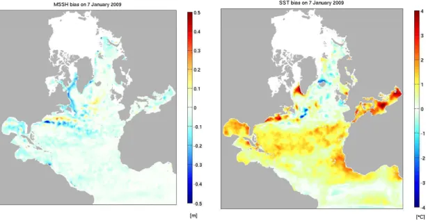
1. The bias fields for each ensemble member are initialised to random spatially uni-form values, with the standard deviation of the order of expected bias magnitude (the SST bias fields were initialised in the interval [−4,4]◦C; the MSSH bias fields – [−0.6,0.6] m). There is no need to have spatial variations in the initial fields due
5
to the use of localisation.
2. These fields are then augmented to the state vector.
3. During assimilation, the forecast observations for each ensemble member are offset by the value of the corresponding bias field. This involves SLA and SST ob-servations, as well as in-situ temperature obob-servations, which are offset up to the
10
model depth of the mixed layer for a given ensemble member, with a smooth tran-sition between offsetting by the full magnitude of the SST bias and no correction at about the mixed layer depth.
4. The bias fields are corrected due to their correlations with the forecast ensemble observations, which establish after a few assimilation cycles.
15
5. The bias fields remain constant during propagation, but their spread reduces after each assimilation cycle. Therefore, to avoid collapse of bias field ensembles, additional inflation is introduced (2 % per cycle for SLA, and 6% for SST).
This bias estimation procedure is similar to that in the EnKF-Matlab package available from http://enkf.nersc.no/Code/EnKF-Matlab.
20
The difference in the magnitude of inflation for the SST and MSSH bias field is due to the fact that, as indicated by the innovation statistics, the SST bias has seasonal variability; while SLA is supposed to have substantial constant or interseasonal com-ponent.
Note that the bias correction doesn’t explicitly correct the model bias, but rather
25
OSD
9, 1519–1575, 2012TOPAZ4 system
P. Sakov et al.
Title Page
Abstract Introduction
Conclusions References
Tables Figures
◭ ◮
◭ ◮
Back Close
Full Screen / Esc
Printer-friendly Version Interactive Discussion
Discussion
P
a
per
|
Dis
cussion
P
a
per
|
Discussion
P
a
per
|
Discussio
n
P
a
per
|
plus the diagnosed time-dependent bias. Also note that in TOPAZ4 the bias estimates are subtracted from the innovation, so that a well-behaved bias estimate reduces, on average, the innovation magnitude.
5 Results
5.1 Innovation statistics 5
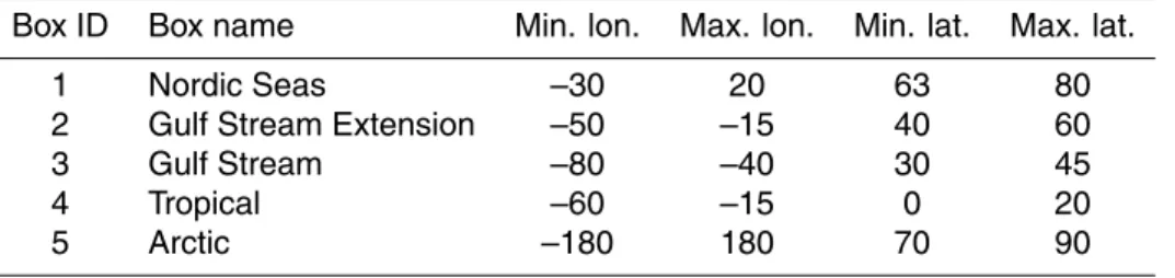
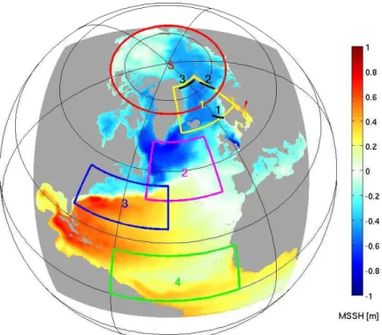
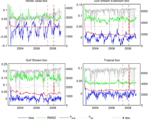
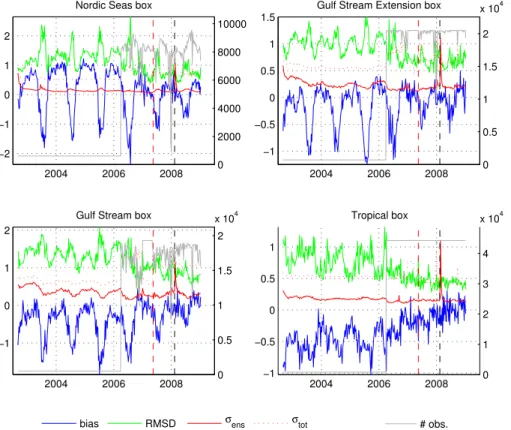
The background innovation is a vector of differences between the observations and the model estimate of the observed quantities immediately before an assimilation is performed. Time series of the background innovation statistics, averaged over different regions (see Fig. 1 and Table 2), are shown for SLA (Fig. 5), SST (Fig. 6), and ICEC (Fig. 7). In each case, time series are shown for the model bias (labelled bias); the
10
root-mean-squared difference (RMSD) between the observations and the model back-ground field (labelled RMSD); the standard deviation of ensemble anomalies (labelled
σens) that represents an estimate of the background error standard deviation; the
es-timated standard deviation of the innovation (labelledσtot) that is the quadrature sum
ofσens and the assumed observation error standard deviation σobs; and the number
15
of observations to be assimilated (labelled # obs.).
Note that the RMSD and the bias are not independent (Oke et al., 2002). For dif-ferent applications, different components of the RMSD might be more important. For example, the bias might be most informative for the assessment of sea ice extent and the freezing and melting of sea ice; while the correlation might be most informative for
20
the assessment of eddies and meanders, where the “shape” and phase of features in the ocean are important.
The time series of the innovation statistics for SLA (Fig. 5) show that the RMS of the innovations remained fairly constant throughout the reanalysis. These time series indicate that the RMS error for SLA is about 0.05 m in the Nordic Seas box; between
25
OSD
9, 1519–1575, 2012TOPAZ4 system
P. Sakov et al.
Title Page
Abstract Introduction
Conclusions References
Tables Figures
◭ ◮
◭ ◮
Back Close
Full Screen / Esc
Printer-friendly Version Interactive Discussion
Discussion
P
a
per
|
Dis
cussion
P
a
per
|
Discussion
P
a
per
|
Discussio
n
P
a
per
|
Gulf Stream box; and about 0.04 m in the Tropical box. We note a substantial seasonal bias in the Nordic Seas box, and to a lesser degree, in the Gulf Stream Extension box. The SLA innovation bias in the Nordic Seas box seems to exceed, on average, the estimated amplitude of seasonal steric height anomaly in the Nordic Seas (Siegismund et al., 2007, Figure 5).
5
Generally, there is a good agreement between the estimated innovation standard deviationσtot and the measured RMSD for all presented fields. This demonstrates an internal consistency between the background and observation error variance and the innovations.
With regard to the innovation statistics for SST (Fig. 6), the RMSD of the innovations
10
fluctuate throughout the period of the reanalysis, with a peak each year that corre-sponds to a peak in the magnitude of the bias. This seasonal behaviour of the bias and RMSD is clearly seen in all boxes, except, perhaps, the Tropical box where the sea-sonality is weaker. The magnitude of the bias and the RMS are often comparable. This indicates that the RMSD between the reanalysed and observed SST is often dominated
15
by the bias. In February 2006, the assimilated SST data was switched from Reynolds SST to OSTIA. The timing of this switch is evident in Fig. 6, when the number of ob-servations increases significantly. The RMSD and bias decrease after this transition, indicating that the OSTIA SST is better suited to constraining the TOPAZ system. Prior to 2006, the RMS of the SST innovations in the Nordic Seas, Gulf Stream Extension,
20
Gulf Stream and the the Tropical boxes is typically between 1.1–1.8◦C, 0.7–1.2◦C, 1– 1.5◦C, and 0.6–1.0◦C respectively. After OSTIA SST data started to be assimilated the RMSD of the SST innovations dropped to 0.5–0.8◦, 0.5–1.0◦ (with the exception of the peak in summer 2006), 0.7–1.3◦C, and 0.4–0.5◦C in the Nordic Seas, Gulf Stream Extension, Gulf Stream, and Tropical boxes respectively.
25
OSD
9, 1519–1575, 2012TOPAZ4 system
P. Sakov et al.
Title Page
Abstract Introduction
Conclusions References
Tables Figures
◭ ◮
◭ ◮
Back Close
Full Screen / Esc
Printer-friendly Version Interactive Discussion
Discussion
P
a
per
|
Dis
cussion
P
a
per
|
Discussion
P
a
per
|
Discussio
n
P
a
per
|
after this point in the Gulf Stream and Tropical boxes, and decreases to some degree in the Nordic Seas and Gulf Stream Extension boxes; the RMS of the innovations also reduces after the bias is explicitly diagnosed and accounted for. Interestingly, the SST bias field does not show as much seasonal variability (not shown) as the bias of the SST innovations. This suggests that the seasonality of the SST bias that is evident in
5
Fig. 6 may be related to the seasonal variations in the surface mixed layer depth. The surface mixed layer is generally deeper in winter. This is reflected in the ensemble-based background error covariance (not shown) that projects the SST innovations over a greater depth in winter. As a result, during winter, it appears that the assimilation of SST data better constrains the ocean model.
10
The vertical dashed red line in Fig. 6 denotes the time when the variance increasing factor of 2 for the update of the ensemble anomalies, described in Section 3.2, was introduced. It is expected to result in the increase of the ensemble spread and therefore the sensitivity of the DA system to observations. The impact on the ensemble spread is evident in Figs. 5 and 6, but any change in the sensitivity of the analysis system to
15
individual observations is less clear. We suspect a parallel run without the variance increasing factor is needed to quantify this sensitivity.
The ensemble spread for SST remains relatively constant throughout the reanalysis for all domains considered here, indicating that the DEnKF showed no tendency to-wards ensemble collapse. It shows some seasonal fluctuations in each box except the
20
Tropical box, with greater spread in winter and less in summer.
For an optimal data assimilation system,σtot should match the RMS of the innova-tions. Clearly, for SST prior to the switch to OSTIA SST, σtot was too small by about 50 % of the RMS, but was approximately correct after the switch to OSTIA. This indi-cates that either the ensemble spread,σens, was too small before the switch to OSTIA,
25
OSD
9, 1519–1575, 2012TOPAZ4 system
P. Sakov et al.
Title Page
Abstract Introduction
Conclusions References
Tables Figures
◭ ◮
◭ ◮
Back Close
Full Screen / Esc
Printer-friendly Version Interactive Discussion
Discussion
P
a
per
|
Dis
cussion
P
a
per
|
Discussion
P
a
per
|
Discussio
n
P
a
per
|
the background fields in the reanalysis.
The time series of the innovation statistics for ICEC is shown in Fig. 7. The most notable feature in the time series of RMSD is the peaks each summer. This occurs because summer is the period when sea ice variability is highest. At the start of sum-mer, sea ice melts and at the end of summer it begins to freeze. The timing of this
5
melting and freezing each summer can be seen in Fig. 7 when the number of observa-tions assimilated substantially decreases and then increases again, reflecting the ice extent. Note the strong correlation between the RMSD and the bias. This indicates that a significant portion of the RMSD is attributed to the bias.
The vertical dashed black line marks the time when a number of changes have been
10
introduced into the system after observing some excessive increments in salinity in the course of assimilating ICEC. These changes include the introduction of adaptive observation pre-screening (Sect. 4.2), increasing the perturbations of model forcing to affecting the position of the ice edge (Sect. 3.3), and relaxation of the assumed ob-servation error variance (Sect. 4.2). These changes seem to improve the performance
15
of the system in regard to the ICEC. For example, there is an increasing trend in the RMSD prior to the change, which is then reversed.
The time series of ensemble spread shows a peak each summer that is in phase with the peak in RMSD. Moreover, the time series of the estimated standard deviation of the innovationσtot is remarkably well-aligned with the RMSD.
20
This demonstrates an internal consistency between the actual errors, quantified by the RMSD, and the assumed and modelled estimates of the errors, from the estimated observation errors and the ensemble-based estimate of the background field errors. This is a very encouraging result, because it demonstrates that the time-varying es-timate of the background field errors from the ensemble can be used to quantify the
25
OSD
9, 1519–1575, 2012TOPAZ4 system
P. Sakov et al.
Title Page
Abstract Introduction
Conclusions References
Tables Figures
◭ ◮
◭ ◮
Back Close
Full Screen / Esc
Printer-friendly Version Interactive Discussion
Discussion
P
a
per
|
Dis
cussion
P
a
per
|
Discussion
P
a
per
|
Discussio
n
P
a
per
|
5.2 Bias estimates
The estimated bias fields for MSSH and SST at the end of reanalysis are presented in Fig. 8. An assessment of the bias estimate for MSSH is provided in Fig. 10, where we compare the MSSH derived from TOPAZ before the bias correction is introduced (from a free run of the model), after the bias is introduced (from the reanalysis), and
5
the observations-only MDT from CNES-CLS09 (Rio et al., 2009), not assimilated. The revised MSSH after the bias is introduced is constructed by adding the time-mean estimate of the SSH bias with the MSSH from the free model run. Several aspects of the revised MSSH are in better agreement with CNES-CLS09 MDT than the MSSH from the free model run. For example, the Gulf Stream at Cape Hatteras shoots too far
10
north in the free model run, as one expects from a model of this resolution, is shifted southwards and is more confined in the revised MSSH. The improvement is visible in the meridional section at 60 W in Fig. 9, where the MSSH drop South of 40 N is sharper after bias estimation and SSH peak on the Southern side of the Gulf Stream is also reproduced. The correlation between the model and observations increases from
15
0.71 to 0.74. We also note that the extent of the Sub-polar Gyre in the Labrador Sea is reduced in the revised MSSH, in agreement with the CNES-CLS09 MDT, and the permanent anticyclonic eddy at the Southern tip of the Sub-polar Gyre that is evident in CNES-CLS09 MDT is also evident in the revised MSSH, but is not clear in the original MSSH. Finally, the two branches of NAC inflow into the Nordic Seas are re-equilibrated
20
– the Icelandic branch of the NAC is too strong in the original MSSH. This is also illustrated in the meridional section at 20 W in Fig. 9: the downward slope between 40 N and 60 N is steeper after bias estimation, in better agreement with the observations. Here again, the correlation increases from 0.86 to 0.92.
An attractive aspect of the online bias estimation is that it requires no hand-tuning of
25
OSD
9, 1519–1575, 2012TOPAZ4 system
P. Sakov et al.
Title Page
Abstract Introduction
Conclusions References
Tables Figures
◭ ◮
◭ ◮
Back Close
Full Screen / Esc
Printer-friendly Version Interactive Discussion
Discussion
P
a
per
|
Dis
cussion
P
a
per
|
Discussion
P
a
per
|
Discussio
n
P
a
per
|
The SST bias field (Fig. 8) shows several regions of spatially coherent positive bias, including regions in the Gulf of Mexico and the Caribbean Sea, the Southern part of the sub-Tropical Gyre and parts of the Mediterranean Sea. In these areas the model is warmer, indicating either that the net surface heat flux is too high or that the modelled surface mixed layer is too shallow – so that not enough sub-surface water is entrained
5
into the surface layers. There are also several regions along the path of the Gulf Stream Extension where the SST bias is large and negative. We suspect that this is an indication that the path of the Gulf Stream is too far to the South.
5.3 Comparison with drifting buoys
A series of SSH maps for different seasons is presented in Fig. 11 with drifter
trajecto-10
ries overlaid. In each map, we show the position of all available drifters, obtained from http://www.meds-sdmm.dfo-mpo.gc.ca/isdm-gdsi/drib-bder/svp-vcs/index-eng.asp on 3 March 2011. Each map in Fig. 11 shows daily averaged SSH and 6-hourly drifter positions for a 9-day window centred on the model time. The purpose of this analy-sis is to provide an independent qualitative assessment of the mesoscale variability in
15
the reanalysis. Since the ocean circulation is dominated by geostrophy, we expect the drifters to flow along paths of constant SSH, and we hope to see good correspondence between the drifter paths and the mesoscale features in SSH. In most cases, we find that there is good correspondence between the SSH fields in the reanalysis and the independent observations of drifter paths. In many cases, even the details of the drifter
20
paths are well captured by the reanalysis.
The good comparisons between drifter paths and modelled SSH demonstrates that the TOPAZ system produces realistic variability in the North Atlantic Ocean. The good performance of the TOPAZ reanalysis in the North Atlantic confirms that the model is “sufficiently eddy permitting” to provide a realistic representation of the mesoscale
25
OSD
9, 1519–1575, 2012TOPAZ4 system
P. Sakov et al.
Title Page
Abstract Introduction
Conclusions References
Tables Figures
◭ ◮
◭ ◮
Back Close
Full Screen / Esc
Printer-friendly Version Interactive Discussion
Discussion
P
a
per
|
Dis
cussion
P
a
per
|
Discussion
P
a
per
|
Discussio
n
P
a
per
|
We note that a similar comparison between drifter paths and the free running model without data assimilation shows no correspondence between individual mesoscale fea-tures in the model and observations (not shown). This is what we expect, and is a consequence of the chaotic nature of mesoscale variability. Individual eddies and me-anders spawn from instabilities that are difficult to predict and model explicitly. Although
5
the model may be capable of reproducing eddies and meanders with the right variabil-ity, and in the right locations, without data assimilation it is unable to predict precisely when and where an instability will occur.
5.4 Evaluation of ice fields
The comparisons of early Fall ice thickness in Fig. 12 show that the data assimilation
10
has done limited change to the overall distribution of ice in the Arctic, in line with Lisæter et al. (2003) who found that the assimilation of ice concentrations mostly impacted the position of the ice edge, but not so much the ice volume. As is generally the case when using the EVP rheology, the thick ice covers the whole Beaufort Sea, while the observations of thick ice from ICESat shows it should be more tightly linked to the
15
North of Greenland and the Canadian Archipelago. The assimilation has indeed slightly thickened the ice there, which – by elimination – is likely to be the effect of assimilating ice drift. The ice is also thickened to the North of Franz Joseph Land and Siberian Islands, in better agreement with the ICESAT data, which reflects the better position of the ice edge during the ice minimum.
20
The comparison of the ice drift from TOPAZ with that from IABP buoys and the Tara expedition (not shown) reveals that the model ice drift is generally slightly too fast, by 3 km d−1for slow drift as much as for fast drift, which is a known deficiency of the EVP type of model: Girard et al. (2009) reported an even larger bias of 6 to 7 km d−1. The too fast ice drift is advecting too much ice into the Beaufort Sea and is consistent with
25
OSD
9, 1519–1575, 2012TOPAZ4 system
P. Sakov et al.
Title Page
Abstract Introduction
Conclusions References
Tables Figures
◭ ◮
◭ ◮
Back Close
Full Screen / Esc
Printer-friendly Version Interactive Discussion
Discussion
P
a
per
|
Dis
cussion
P
a
per
|
Discussion
P
a
per
|
Discussio
n
P
a
per
|
5.5 Evaluation of salinity and temperature
Below we will mainly concentrate on the evaluation of salinity, which is the most im-portant tracer for circulation in the Arctic; but we will also provide some temperature comparisons with mooring data.
A comparison of SSS from the TOPAZ reanalysis, from the GDEM climatology
5
(Teague et al., 1990), and from a free run of the model (not shown) indicates that these SSS fields are very similar in the North Atlantic. By contrast, there is a signif-icant improvement in the SSS of the reanalysis in the Arctic compared to that of the free running model.
Figures 13 and 14 show the monthly mean SSS and the monthly mean salinity at
10
100 m depth (S100) for the reanalysis during January 2007, before in situ observations in the Arctic are assimilated, and during January 2008, after in situ observations in the Arctic are assimilated. For comparison, we also show an estimate of SSS climatology from PHC (Steele et al., 2001).
The SSS and S100 fields in January 2007, before in situ observations in the Arctic
15
are assimilated, show an unrealistically large and misplaced Beaufort Gyre, with too low salinity. The salinity of the free run is very similar to that of the reanalysis in Jan-uary 2007 (not shown). In spite of this model deficiency, the intensity and location of the Beaufort Gyre are corrected efficiently by assimilation of the profiles. We interpret this improved performance in 2008 as an indication that the assimilation of in situ
ob-20
servations in the Arctic is beneficial, and has had a measurable positive impact on the reanalysis (however, see Sect. 5.8 in regard to the patchiness observed in the middle panels of Figs. 13 and 14).
In particular, the assimilation of ITP profiles appears to be critical for constraining the central Arctic temperature and salinity structures, even though the number of ITP
25
OSD
9, 1519–1575, 2012TOPAZ4 system
P. Sakov et al.
Title Page
Abstract Introduction
Conclusions References
Tables Figures
◭ ◮
◭ ◮
Back Close
Full Screen / Esc
Printer-friendly Version Interactive Discussion
Discussion
P
a
per
|
Dis
cussion
P
a
per
|
Discussion
P
a
per
|
Discussio
n
P
a
per
|
reanalysis.
The temperature and salinity profiles in the Arctic are assessed against the NA-BOS/CABOS moorings in Fig. 15. The moorings were active before the assimilation of ITP data but not assimilated. The temperature profiles in the Laptev Sea reveal in-sufficient transport or excessive diffusion of warm Atlantic Water. Although transport
5
estimate in the Fram Strait compares well with observations(see Sect. 5.7), the core of Atlantic Water is too weak and too diffuse (see Sect. 5.6). This excessive diff u-sion may result from the artificial thickness diffusion used for model stability or from our parametrisation of diapycnal mixing that does not account for the attenuation of internal waves below sea ice (Morison et al., 1985; Nguyen et al., 2009).
10
For the Canadian mooring the comparison with observations for both the reanalysis and the free run is quite poor. Note, however, that historically TOPAZ has been cali-brated for the North Atlantic and the adjacent Arctic sector rather than for the Canadian basin. Both simulations show a too shallow and too cold Pacific Water, which is likely to be a direct consequence from dis-regarding seasonal variability in the Bering Strait
15
inflow. The reanalysis does not show the Atlantic layer presented in observations, and in this instance, the free running model is closer to observations. However, in view of the relatively patchy horizontal fields (not shown), we suspect the deterioration of the reanalysis to be an isolated case rather than reflecting a general tendency.
5.6 Comparison with hydrographic sections 20
The Fram Strait is the main oceanic gateways between the Atlantic and the Arctic ocean and is thus the most important region for the exchange of Atlantic and Polar water masses. Since 1997 oceanic fluxes through Fram Strait have been monitored by an array of moorings deployed between 6◦30′W and 8◦40′E at the latitude 78◦50′N (Schauer et al., 2008; Beszczynska-M ¨oller et al., 2011). This data-set is not assimilated
25
OSD
9, 1519–1575, 2012TOPAZ4 system
P. Sakov et al.
Title Page
Abstract Introduction
Conclusions References
Tables Figures
◭ ◮
◭ ◮
Back Close
Full Screen / Esc
Printer-friendly Version Interactive Discussion
Discussion
P
a
per
|
Dis
cussion
P
a
per
|
Discussion
P
a
per
|
Discussio
n
P
a
per
|
On the western side the East Greenland Polar front englobe the fresh and cold Polar Water. Between 800 m and 1200 m, one can find the Arctic Intermediate Water and the Upper Polar Deep Water with a temperature close to 0◦C. Bellow, the Nordic Sea Deep Water and the Arctic Ocean Deep Water are present.
Figure 16 compares temperature from the free and assimilative runs to the data in the
5
Winter and Summer 2007. The improvements from data assimilation are numerous. The Atlantic Water in the free run is too cold, too deep and diffuse. This is much improved in the reanalysis even if the multiple cores are not clearly represented and the core of Atlantic Water is still too deep and slightly too diffuse. The Polar Water is also too deep in the free run. In the reanalysis the water is located at a reasonable
10
depth but extends too far to the East. Both the free run and the reanalysis misrepresent the deep water. The differences in the intermediate and deep water are small, but the stratification is better pronounced in the reanalysis and the deep water is slightly colder. It appears that the influence of data assimilation at depths is minor.
It is worth mentioning that the comparison in the Fram Strait is affected by the
ini-15
tialisation problem described in Sect. 5.8. In a normal free run (initialised from a long spin-up), the water masses are in better agreements to observations than in the free run started from the ensemble mean.
5.7 Volume transport estimates
Time series of 3-monthly averaged volume transports through the Svinøy section and
20
Barents Sea Opening (denoted in Fig. 1), from the reanalysis and from independent observations, is presented in Fig. 17. The Svinøy section is a key location for mea-suring the Atlantic inflow to the Norwegian Sea, due to the topographic steering of the Norwegian Atlantic Slope Current (NwASC) and its vertical structure. Skagseth et al. (2008) estimate the volume flux from one single mooring in the core of the flow.
25
OSD
9, 1519–1575, 2012TOPAZ4 system
P. Sakov et al.
Title Page
Abstract Introduction
Conclusions References
Tables Figures
◭ ◮
◭ ◮
Back Close
Full Screen / Esc
Printer-friendly Version Interactive Discussion
Discussion
P
a
per
|
Dis
cussion
P
a
per
|
Discussion
P
a
per
|
Discussio
n
P
a
per
|
of moored current measurements in the BSO monitors the fluxes between Norway and Bear Island (Ingvaldsen et al., 2004). The associated uncertainty estimates are not provided in either case, but differences should be expected between the punctual current measurements and the section-averaged volume fluxes, even after low pass filtering. The velocity measurements used to generate the observational estimates of
5
the volume transport in Fig. 17 were not assimilated in the reanalysis.
In the Svinøy section the transport estimate from the free run is too low (3.5 Sv) compare to observation (4.7 Sv) and the one from the reanalysis is too high (6.1 Sv). The free run transport is too low until 2005, but then adjusts to a level that is compa-rable to the observation while the reanalysis transport remains offset during the whole
10
integration. The variability is relatively well captured by the model but the reanalysis correlates better with the observations, with the correlation coefficient increasing from 0.7 to 0.8. Both model runs represents reasonably well the seasonal variably but the interannual variability of the volume transports is better reproduced by the reanalysis with an increasing trend until 2006, followed by a decreasing trend.
15
In the BSO, the interannual variability is missing, and the model does not represents the very high maximum in 2006 nor the decreasing trend, and the correlation is poor (0.42 for the reanalysis and 0.40 for the free run). We attribute this difference to insuffi -cient resolution in the surface forcing fields (from ERA-interim) that does not accurately represent winter storms and polar lows. The transport is overestimated in both the free
20
run and the reanalysis (with 2.9 Sv instead of 2.2 Sv from observations). Still, the free and assimilated run are very close to each other and reasonably close to the obser-vations with respect to other model products of higher resolution (Gammelsrød et al., 2009).
Finally, the transport in the Fram Strait is analysed against the estimate from
Mau-25