A synthesis of marine sediment core δ<sup>13</sup>C data over the last 150 000 years

(1)

CPD

5, 2497–2554, 2009

Synthesis of marine

δδδ13C

K. I. C. Oliver et al.

Title Page

Abstract Introduction

Conclusions References

Tables Figures

◭ ◮

Back Close

Full Screen / Esc

Printer-friendly Version

Interactive Discussion

Clim. Past Discuss., 5, 2497–2554, 2009 www.clim-past-discuss.net/5/2497/2009/

Climate of the Past Discussions

This discussion paper is/has been under review for the journal Climate of the Past (CP). Please refer to the corresponding final paper in CP if available.

A synthesis of marine sediment core

δ

13

C

data over the last 150 000 years

K. I. C. Oliver1,2, B. A. A. Hoogakker3, S. Crowhurst3, G. M. Henderson4, R. E. M. Rickaby4, N. R. Edwards1, and H. Elderfield3

1

Department of Earth and Environmental Sciences, The Open University, Walton Hall, Milton Keynes MK7 6AA, UK

2

School of Ocean and Earth Science, National Oceanography Centre, University of Southampton, European Way, Southampton SO14 3ZH, UK

3

Department of Earth Sciences, University of Cambridge, Downing Street, Cambridge CB2 2EQ, UK

4

Department of Earth Sciences, University of Oxford, Parks Road, Oxford OX1 3PR, UK

Received: 19 November 2009 – Accepted: 21 November 2009 – Published: 11 December 2009

Correspondence to: K. I. C. Oliver (k.i.c.oliver@noc.soton.ac.uk)

(2)

CPD

5, 2497–2554, 2009

δδδ13C

Title Page

Tables Figures

◭ ◮

Back Close

Full Screen / Esc

Interactive Discussion Abstract

The isotopic composition of carbon, δ13C, in seawater is used in reconstructions of ocean circulation, marine productivity, air-sea gas exchange, and biosphere carbon storage. Here, a synthesis ofδ13C measurements taken from foraminifera in marine sediment cores over the last 150 000 years is presented. The dataset comprises previ-5

ously published and unpublished data from benthic and planktonic records throughout the global ocean. Data are placed on a commonδ18O age scale and filtered to remove timescales shorter than 6 kyr. Error estimates account for the resolution and scatter of the original data, and uncertainty in the relationship betweenδ13C of calcite and of dissolved inorganic carbon (DIC) in seawater. This will assist comparison with δ13C 10

of DIC output from models, which can be further improved using model outputs such as temperature, DIC concentration, and alkalinity to improve estimates of fractionation during calcite formation.

High global deep oceanδ13C, indicating isotopically heavy carbon, is obtained dur-ing Marine Isotope Stages (MIS) 1, 3, 5a, 5c and 5e, and lowδ13C during MIS 2, 4 15

and 6, which are temperature minima, with larger amplitude variability in the Atlantic Ocean than the Pacific Ocean. This is likely to result from changes in biosphere carbon storage, modulated by changes in ocean circulation, productivity, and air-sea gas ex-change. The North Atlantic verticalδ13C gradient is greater during temperature minima than temperature maxima, attributed to changes in the spatial extent of Atlantic source 20

waters. There are insufficient data from shallower than 2500 m to obtain a coherent pattern in other ocean basins. The data synthesis indicates that basin-scaleδ13C dur-ing the last interglacial (MIS 5e) is not clearly distdur-inguishable from the Holocene (MIS 1) or from MIS 5a and 5c, despite significant differences in ice volume and atmospheric CO2concentration during these intervals. Similarly, MIS 6 is only distinguishable from 25

(3)

CPD

5, 2497–2554, 2009

δδδ13C

Title Page

Tables Figures

◭ ◮

Back Close

Full Screen / Esc

number of records.

1 Introduction

The isotopic composition, δ13C, of inorganic carbon in seawater is a diagnostic of ocean circulation and the marine and terrestrial carbon cycle. The potential forδ13C in calcium carbonate shells, formed by foraminifera and preserved in marine sediments, 5

to record past changes in climate has been recognised since the 1970s (Shackleton, 1977; Duplessy et al., 1981). Greater differences in δ13C between planktonic and benthic foraminifera, during glacial periods, were interpreted as indicating greater stor-age of isotopically light organic carbon in the deep ocean and linked to atmospheric pCO2(Broecker, 1982a; Shackleton et al., 1983; Shackleton et al., 1992). Lowerδ

13 C 10

values recorded in the Pacific Ocean, during the last glacial maximum (LGM), were attributed to a change in the oceanδ13C reservoir due to the release of organic carbon from the terrestrial biosphere or marine shelf sediments (Broecker, 1982b; Duplessy et al., 1988b). Carbon isotopes have also been used to reconstruct past water masses, notably lowδ13C Antarctic source waters and highδ13C Atlantic source waters (Sarn-15

thein et al., 1994), or to diagnose changes in air-sea gas exchange (Marchitto and Broecker, 2006). However, the interpretation of the δ13C is complicated by the de-pendence of fractionation during calcification on properties of the water (temperature; [CO2]; [CO

2−

3 ]) and the foraminifer (species; shell size; diet), and on the formation of microenvironments around benthic foraminifera (Sect. 3). The variety of mechanisms 20

influencing theδ13C record is summarised in Fig. 1.

The reconstruction of past ocean states depends on the collation ofδ13C observa-tions from throughout the ocean, which can provide a fairer test to hypotheses than individual datasets. The demand for such syntheses is increased by the development of Earth system models that are able to simulate paleoclimate proxies includingδ13C 25

(4)

CPD

5, 2497–2554, 2009

δδδ13C

Title Page

Tables Figures

◭ ◮

Back Close

Full Screen / Esc

Bickert and Mackensen, 2003; Curry and Oppo, 2005; Lynch-Stieglitz et al., 2007), typically focusing on the difference between the late Holocene and the LGM. Data from the benthic speciesCibicidoides wuellerstorfi, considered the most reliable indicator of seawaterδ13C, were selected for those time-slices, reducing the error in the data at the expense of reduced data coverage. In this study, we focus not on specific times-5

lices but on producing a synthesis of timeslices, at 2 kyr intervals, for the last 150 kyr. We include data from a range of benthic and planktonic species, and do not exclude data from high productivity regions. The inhomogeneity in this data is addressed by attaching an error estimate for each observation, using the entire dataset to estimate additional errors associated with less reliable species and unfavourable core locations. 10

The goals for this study are threefold: (1) to provide a common δ18O-derived age-scale for a synthesis ofδ13C data; (2) to provideδ13C error estimates for the synthesis, in order to facilitate direct model–data comparison; (3) to provide a global overview of the data, and an account of the large scale processes invoked to explain changes in ocean δ13C. In Sect. 2, we introduce the data and summarise the age-scale intro-15

duced in the companion paper (Hoogakker et al., 2009a). In Sect. 3, we describe the methods used to determine uniformly spaced time-series and uncertainty intervals. In Sect. 4, we examineδ13C time-series, grouped by region, and six time-slices, as well as planktonic-benthic differences. We summarise our findings in Sect. 5, and discuss their application for Earth System models and biosphere reconstructions.

20

2 Data

2.1 Data selection and coverage

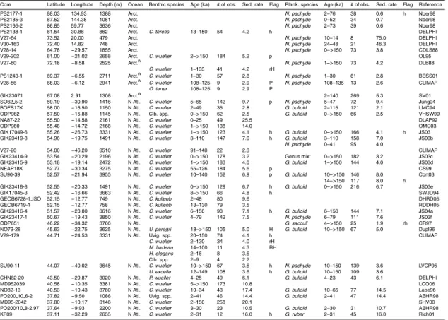
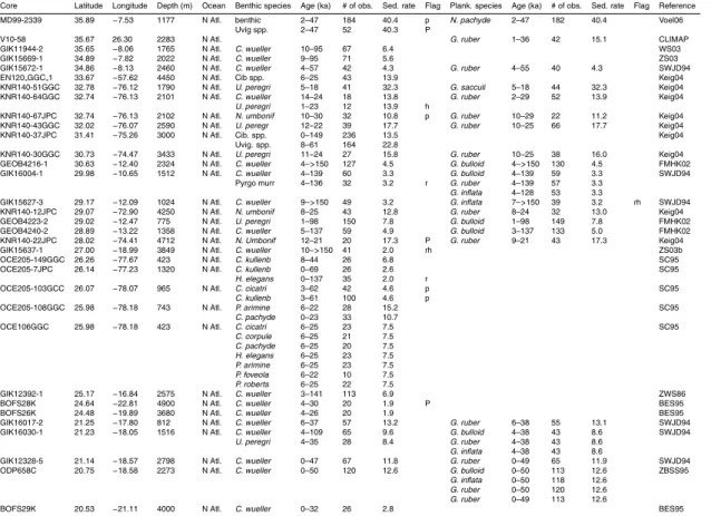
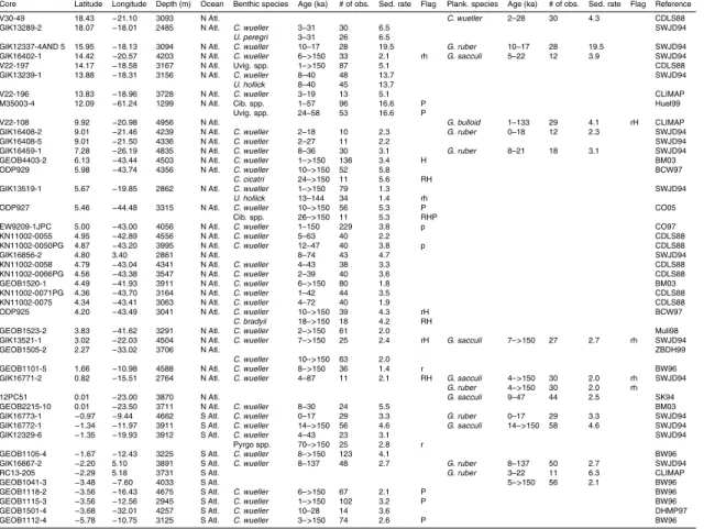
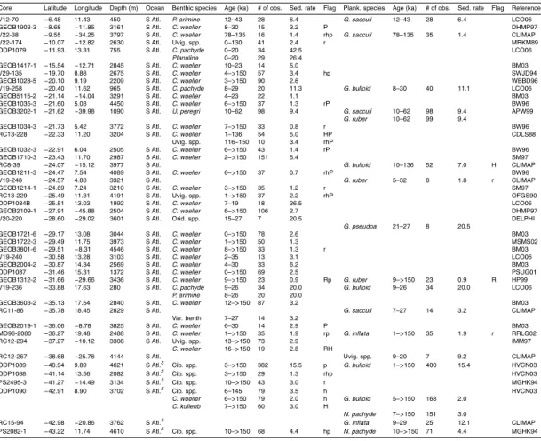
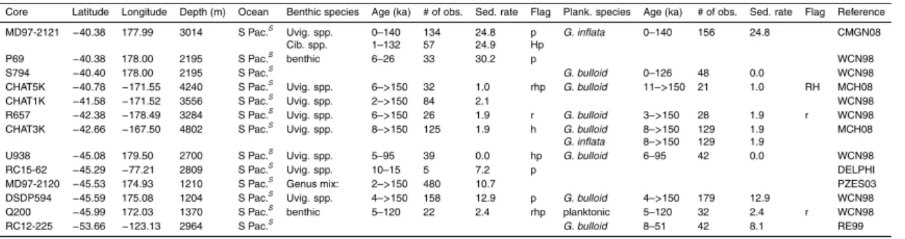
Table 1 summarises the data used in this compilation. Data consist mostly of records submitted to the PANGAEA publishing network for geoscientific and envi-ronmental data (http://pangaea.de), the National Geophysical Data Centre (NGDC; 25

(5)

CPD

5, 2497–2554, 2009

δδδ13C

Title Page

Tables Figures

◭ ◮

Back Close

Full Screen / Esc

with additional records obtained through personal correspondence.δ13C records were accepted into the pre-processed compilation provided that it was possible to obtain a reliable (though sometimes low resolution) age model within the last 150 000 years usingδ18O stratigraphy (Hoogakker et al., 2009a). No data quality constraint was ap-plied to the pre-processed compilation, but several factors (detailed in Sect. 3) can lead 5

to a large error estimate, so that some data were ultimately rejected as having too large an associated error to be useful.

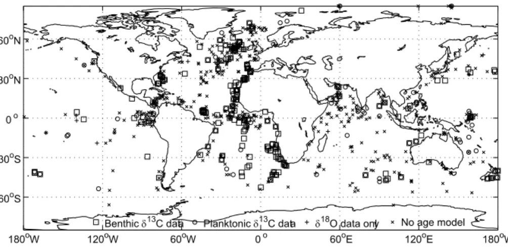
Figure 2 shows the core locations for the records used in the data synthesis, as well as for records for which we were unable to provide aδ18O–derived age model. Among the records that were used, there is good data coverage in deep waters (>2500 m) in 10

the Atlantic Ocean (100 cores with benthic data). Atlantic data coverage is also rea-sonable at shallower depths (45 cores) and in surface waters (71 cores with plank-tonic data). The principal gaps in benthic data coverage are: (1) <2500 m in the Pacific ocean (10 cores); (2) the Indian ocean (12 cores); and (4) south of 50◦S (2 cores). There is a large variation in the temporal resolution of the pre-processed data, 15

both within and across cores. Of the cores providing benthic data, all but 28 vide at least one observation for the LGM (19–23 ka), compared with 64 cores pro-viding no Holocene (<10 ka) data, and 124 cores providing no data from Marine Iso-tope Stage (MIS) 5a or earlier (>71 ka). This is summarised in Table 1. The data, pre-processed onto a δ18O age-scale and with a limited amount of filtering (the ex-20

clusion of small subsets of data taken from a different species to the majority of the record) but with no changes toδ13C values, are available from the authors. We cau-tion that these data do not constitute a repository of raw records, which can instead be obtained from PANGAEA, NGDC, or Delphi. The fully processed data, after ap-plying the methods described in Sect. 3, are included as Supplementary Materials 25

(6)

CPD

5, 2497–2554, 2009

δδδ13C

Title Page

Tables Figures

◭ ◮

Back Close

Full Screen / Esc

2.2 Age modelling

A detailed description of the age modelling method is provided in the companion paper (Hoogakker et al., 2009a). In summary,δ18O data, obtained together withδ13C data, were used to manually obtain pivot dates at 18 ka, 62 ka, 87 ka, 108 ka, and 137 ka. It was assumed that these dates correspond to local maxima in theδ18O time-series. 5

The selection of these pivot dates was constrained by a subjective judgement of plau-sible age-depth relationships; large changes in mean sedimentation rate between pivot dates were considered unlikely, though not impossible. Between pivot-points, a uniform sedimentation rate was assumed. For high resolution records where pivot dates could be clearly identified, we estimate 2σ uncertainties associated with this approach of up 10

to 6 kyr between pivot dates (excluding uncertainties in the initial selection of dates of δ18O maxima). Lower resolution cores, cores with low resolution segments (see Ta-ble 1), or cores with hiatuses, are likely have greater dating uncertainties. Therefore inter-basin differences in the timing ofδ18O changes (Skinner and Shackleton, 2005) are unlikely to be a major additional source of dating error. The age models presented 15

are not suitable for examining the detailed phasing of changes inδ13C within deglacia-tions, or for events with timescales close to that of ocean circulation, but are suitable for examining variability on orbital timescales.

Earlier published or unpublished age models, based on a variety of methods includ-ing radiocarbon datinclud-ing and stratigraphy, were also obtained for many of the records. In 20

(7)

CPD

5, 2497–2554, 2009

δδδ13C

Title Page

Tables Figures

◭ ◮

Back Close

Full Screen / Esc

Interactive Discussion 3 Procedure for temporal gridding andδδδ13C uncertainty estimation

This section describes the treatment of data inhomogeneity within and between records in obtaining a temporally gridded data synthesis, with uncertainties ascribed to individ-ual δ13C values as a function of species, core location, data resolution and scatter. In accounting for data inhomogeneities, it is useful to distinguish between systematic 5

errors associated with each record (intrecord error) and the temporally varying er-ror component (intra-record erer-ror). For example, the erer-ror due to fractionation during calcification has a large inter-record component because this is strongly dependent on species, and most records consist of samples from a single species or genus. Spatial variability in the species offset is also an inter-record error, but in situ variability of this 10

offset in response to climate change is an intra-record error. Similarly, any systematic difference inδ13C resulting from intlaboratory calibration errors is an intrecord er-ror. Since we expect uncertainties in the systematic inter-record error to be significant, δ13C and its uncertainties are estimated by two stages. First, we present intra-record variability inδ13C relative to the LGM, which we label∆LGMδ

13

C (Sect. 3.1). Second, 15

we obtain estimates for absolute δ13C values (Sect. 3.2). ∆LGMδ 13

C can be used to understand spatial patterns inδ13C variability, and has smaller uncertainty than abso-luteδ13C. Therefore, we recommend that∆LGMδ

13

C is chosen where possible when using this data synthesis (for example for model-data comparison), and it is also the variable presented in most figures within this paper.

20

3.1 Obtainingδδδ13C as anomalies relative to the LGM

∆LGMδ 13

C is temporally gridded at 2 kyr intervals, and the smoothing spline applied to the data approximates a 6 kyr low pass filter (Sect. 3.1.1), removing high frequency variability such as Dansgaard-Oeschger oscillations which are beyond the precision of the age model. All∆LGMδ

13

C values are calculated as an anomaly relative to the 25

(8)

CPD

5, 2497–2554, 2009

δδδ13C

Title Page

Tables Figures

◭ ◮

Back Close

Full Screen / Esc

definition of 19–23 ka (e.g. Bickert and Mackensen, 2003; Paul et al., 2009); averaging pre-processed data within the 19–23 ka interval would not be preferable due to uncer-tainties in the age model. The LGM, rather than the late Holocene, is chosen as the reference period because almost all cores provide LGM data, whereas approximately half of all cores provide no data for<4 ka.

5

Three steps were taken to obtain∆LGMδ 13

C estimates and uncertainties, described in detail below. First, each time-series was smoothed and gridded, and the error as-sociated with this process estimated (Sect. 3.1.1). Second, a correction and additional error was estimated for cores thought to be subject to changes in the phyto-detritus effect (Sect. 3.1.2). Third, an error for the representativeness of each species of the 10

ambient water was estimated (Sect. 3.1.3). Although the errors associated with each of these steps are likely to be correlated, there were insufficient data to reliably estimate these correlations, so the total error was estimated to be the quadratic sum of the error components. 2σerror estimates are quoted; where they exceed 1‰ or where the data resolution is poorer than 6 kyr, no final∆LGMδ

13

C estimate is given. Full error estimates 15

are provided as part of the uniformly spaced output dataset (Supplementary Materials http://www.clim-past-discuss.net/5/2497/2009/cpd-5-2497-2009-supplement.zip).

3.1.1 Smoothing splines

The first step in obtaining∆LGMδ 13

C estimates was independent of species or region, and a function only of the input time-series data. These were smoothed and placed on 20

a uniform 2 kyr grid using the spline smoothing method described by Silverman (1985). For a time-series ofnobservations, the set ofn−1 cubic equations was obtained which minimised

θ=λ

Zt_n

t₁ ¨ y2_d_t

+n−1

Σn_i₌₁y′2

i , (1)

whereλis the smoothing parameter,y is the outputδ13C estimate and ¨y is its second 25

(9)

CPD

5, 2497–2554, 2009

δδδ13C

Title Page

Tables Figures

◭ ◮

Back Close

Full Screen / Esc

of each record (note thatt is defined positive towards the past), andy′ is given by

y_i′2=(yi−Yi)2, |yi−Yi|≤ythr,

y_i′2=y_thr2 +|yi−Yi| −ythr, |yi−Yi| > ythr, (2) whereY_i is theδ13C observation andy_thr=0.5‰ was chosen to prevent outliers from having a dominant effect on the estimate (Enting, 1987). The smoothing parameter is 5

given by

λ= (n−1)T 4 0.5 (2π)4₍_t

n−t1)

, (3)

where T0.5 was chosen to be 6 kyr. For a uniformly spaced input time-series, this method is equivalent to a kernel filter admitting 50% of variability with a period ofT0.5, steeply increasing towards 100% at longer timescales and steeply decreasing towards 10

0% at shorter timescales (Enting, 1987). For time-series with non-uniformly spaced data, the period at which 50% of the variability is admitted is a weak function (∼fˆ−14₎

of the local kernel density ˆf. Kernel data density estimates, which approximate to the inverse of the temporally local data resolution∆t, are provided as part of the uniformly spaced output dataset (Supplementary Materials http://www.clim-past-discuss.net/5/ 15

2497/2009/cpd-5-2497-2009-supplement.zip).

A first estimate of the error in the smoothed time-series is given by (Silverman, 1985)

2σsil(t)=2 4λ

1 3fˆ(t)−

3 8

_Σn

i=1y

′2 i

n34−2−32λ−14Σn

i=1fˆ(ti)

12

. (4)

Typical values of 2σsil are of the order of 0.1‰, rarely increasing above 0.25‰. How-ever, this method is intended for time-series with largen, and unrealistically small error 20

(10)

CPD

5, 2497–2554, 2009

δδδ13C

Title Page

Tables Figures

◭ ◮

Back Close

Full Screen / Esc

the spectral characteristics of both the signal and the noise. For our purposes, all high frequency variability is noise, and it is likely that this is aliased in low resolution time-series. In order to address this, we assume that the root-mean-square of the residuals,

¯

y′_{, from high resolution time-series provides an estimate of the noise present in all} time-series. Where smaller values of ¯y′ _{are obtained from low resolution records, this}

5

indicates that variability in the high frequency (T <T_0.5) band is being aliased as a signal at lower frequencies. ¯y′_{is plotted as a function of time-series mean resolution in Fig. 3,} along with a line of best fit,y_h′, with the form of atanhfunction. We obtain lower values ofy_h′ in low resolution cores. The resulting error estimate due to aliasing,

2σali(∆t)=2 y_h′(0)−y_h′(∆t)

1+ T0 π∆t

−1₂

, (5)

10

is also plotted if Fig. 3. Note that there is a large range in y_h′ even within high fre-quency time-series, likely to be largely caused by data inhomogeneities about which information is often unavailable (e.g. shell sizes used; shells per sample; averaging of duplicate samples). Therefore aliasing error estimates for low resolution time-series are very uncertain. The total error associated with the smoothing spline process is the 15

quadratic sum of 2σsiland 2σali.

3.1.2 Error due to the phyto-detritus effect

A further source of error is the possible change in time of the depositional environment in which benthic foraminifera exist. Infaunal species such as those in the Uvigerina

genus inhabit a microenvironment that is often depleted inδ13C due to the respiration 20

of organic matter in the sediment, whereas δ13C epifaunal species are not typically subject to this effect. There is some evidence that the error in infaunal species varies over a glacial cycle (Hoogakker et al., 2009b), but there are insufficient data to deter-mine a correction that varies over time. In this study, we treat this effect as a constant component of the species offset plus a random error (Sect. 3.1.3); therefore there is no 25

(11)

CPD

5, 2497–2554, 2009

δδδ13C

Title Page

Tables Figures

◭ ◮

Back Close

Full Screen / Esc

Although shells from the epifaunalCibicidoides taxon are thought usually to record theδ13C of ambient water ΣCO2 accurately, several studies have identified a bias to-ward low values in high productivity regions (Mackensen et al., 1993; Sarnthein et al., 1994), termed the phyto-detritus effect. Bickert and Wefer (1999) compared cores from upwelling regions in the Atlantic Ocean to nearby cores outside upwelling regions and 5

found that δ13C in upwelling regions was more depressed, relative to nearby cores, during the LGM than the late Holocene. Bickert and Mackensen (2003) applied a cor-rection of+0.4‰ to LGMδ13C in several upwelling regions in the Atlantic Ocean (parts of the eastern boundary in both hemispheres; equator; subtropical and subantarctic fronts), applying no analogous correction to Holocene values. Such a time-dependent 10

correction influences both δ13C and _∆_LGMδ13C estimates. Figure 4 shows the cor-rection and uncertainty that we add to δ13C estimates in cores, flagged in Table 1, found in the upwelling regions identified by Bickert and Mackensen (2003), including the Antarctic Circumpolar Current. The correction for the LGM is +0.4‰ and for the late Holocene is zero, with an assumed 2σphy error of 0.4‰ at all times. Phyto-detritus 15

corrections, in ‰, throughout the 150 kyr record are given by

δphy(t)=0.4

1− (∆LGMδ

13_C) S1

phy (t)

(_∆_LGMδ13_C) S1

phy (1ka)

, (6)

where (∆LGMδ 13

C)_S1 is the value of∆LGMδ 13

C obtained after spline fitting but before applying the phyto-detritus correction, 1 ka is chosen to represent the late Holocene,

and

phy

indicates averaging over cores for which a phytodetritus correction is ap-20

plied. Values lower than 0‰ or greater than 0.4‰ are replaced with 0‰ and 0.4‰, respectively. Because the LGM is used as the reference date, the correction towards higher values in glacialδ13C corresponds to a correction, towards lower values, in in-terglacial and interstadial ∆LGMδ

13

C (Fig. 4). The 0.4‰ uncertainty is also added to cores at upwelling sites in the Indian and Pacific Oceans (Table 1). However, no correc-25

(12)

CPD

5, 2497–2554, 2009

δδδ13C

Title Page

Tables Figures

◭ ◮

Back Close

Full Screen / Esc

differences at Indo-Pacific upwelling sites to those at nearby sites where there is no upwelling. Therefore, we lack the evidence to support a stronger phytodetritus e_ffect during cold climates in these oceans.

It is not well known to what extent the phyto-detritus effect in epifaunal species is caused by changes in foraminifer growth rate (McConnaughey et al., 1997), or by the 5

build-up of respiring organic matter over epifaunal species leading to a decrease in δ13C similar to that observed in infaunal species. No correlation has been observed between sedimentation rate and amplitude of the phyto-detritus e_ffect, although Mack-ensen et al. (2001) suggested that this is because the key control is seasonal peak de-position rate, rather than annual mean dede-position rate. It is therefore uncertain whether 10

additional errors are introduced to records from infaunal species in high productivity re-gions. As noted above, we apply no correction, but add the same uncertainty as would be added to epifaunal species.

3.1.3 Disequilibria and the calculation of species errors

An important error in_∆_LGMδ13C estimates is variability in disequilibria of δ13C in cal-15

cium carbonate in the shells of foraminifera, relative to the ambient water. Along with the phyto-detritus effect, δ13C disequilibrium leads to the application of different “species o_ffsets” toδ13C data collected from di_fferent species. We note that_∆_LGMδ13C is independent of any uniform species offset, and that errors due to variability between individual shells, or small groups of shells, of a given species have already been implic-20

itly accounted for in the smoothing spline calculation. Of interest here are the causes of variability in the disequilibrium of calcium carbonate through time.

In planktonic formanifiera, recorded δ13C is a strong function of shell size (e.g. Berger et al., 1978; Spero and Lea, 1993; Elderfield et al., 2002), and the difference inδ13C between the largest and smallest size fractions can be greater than glacial-25

(13)

CPD

5, 2497–2554, 2009

δδδ13C

Title Page

Tables Figures

◭ ◮

Back Close

Full Screen / Esc

throughout a record may lead to significant error in ∆LGMδ 13

C. A second source of error is temperature-dependent fractionation, which affects planktonic species due to variability in surface temperature on seasonal to glacial timescales. The temperature-dependence of fractionation is a function of species. Culture experiment estimates of ∂(δ13C)/∂(T) (whereT is temperature) have been made of−0.11‰ ◦C−1for

Globige-5

rina bulloides (Bemis et al., 2000),−0.08‰ ◦C−1 for Limacina inflata (Fischer et al., 1999), 0 to +0.05‰ ◦C−1 for Orbulina universa (Bemis et al., 2000). No relation-ship with temperature was observed onGlobigerinoides ruber (Fischer et al., 1999), whereas Kohfeld et al. (2000) assumed a relationship of−0.13‰ ◦C−1 for Neoglobo-quadrina pachyderma.

10

Culture experiments on planktonic foraminifera also reveal a strong depen-dence on the concentration of the carbonate ion, with a gradient of approximately

−0.012‰/(µmol kg−1) forG. bulloides under constant DIC. Glacial carbonate concen-tration is dependent on the poorly constrained alkalinity inventory of the ocean, but a change of 30 to 80µmol kg−1 is not implausible (Kohfeld et al., 2000), indicating an 15

effect of the same order as glacialδ13C cycles. The effect of carbonate ion on benthic δ13C is not known. A final effect arises due to changes in the isotopic composition of carbon in the diet; culture experiments indicate thatδ13C inG. bulloidesshell carbon-ate varies asδ13C in organic matter in the ratio 0.084:1 (Spero and Lea, 1996).

With the exception of sea-surface temperature reconstructions for the LGM (e.g. 20

MARGO Project Members, 2009), variability in water properties likely to cause system-atic errors in∆LGMδ

13

C are poorly constrained over the last 150 kyr, so no time-varying correction is applied to∆LGMδ

13

C. Therefore, we caution that changes in these prop-erties over a glacial cycle, rather than changes in seawaterδ13C, may contribute sig-nificantly to variability in the the planktonic∆LGMδ

13

C record. However, Earth system 25

(14)

CPD

5, 2497–2554, 2009

δδδ13C

Title Page

Tables Figures

◭ ◮

Back Close

Full Screen / Esc

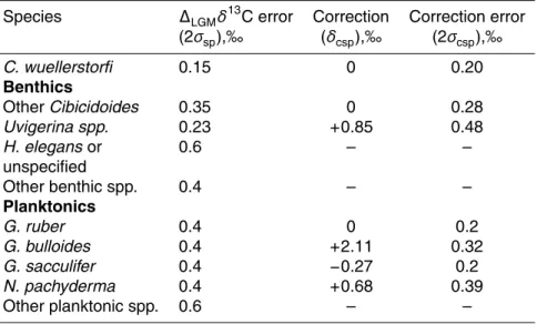
benthicδ13C record.

A random error estimate may be made by comparing records from different species but from the same core. Among benthic species, the epibenthic taxon Cibicidoides wuellerstorfi is widely preferred for recordingδ13C, and to this species we ascribe an error, 2σsp, of 0.15‰. This value is obtained from comparison of water column data 5

(Kroopnick, 1985) with data from core samples (c.f. Beveridge et al., 1995). Error esti-mates for other species in theCibicidoidesgenus were obtained using cores containing both C. wuellerstorfi and another Cibicidoides species. The error is the root-mean-squared (rms) di_fference between the two species after the application of an optimal species offset. This process was repeated for the infaunal genusUvigerina. For other 10

species, there was insufficient overlap in data withC. wuellerstorfito apply this method. For these species, errors of 0.4‰ were ascribed. A larger error of 0.6‰ was applied to data derived fromHoeglandia elegans or from mixed benthics. Error estimates are presented in Table 2.

For planktonic foraminifera, the choice of reference species is less clear. We select 15

G. ruber, which yields data that are consistent on a regional scale, and has a restricted depth range (Fischer et al., 1999), so that changes in recordedδ13C are more likely to reflect changes in surface conditions. We ascribe an error of 0.4‰ to this species, and calculated estimates forG. bulloides, Globigerinoides sacculifer, andN. pachyderma

by the same method used for benthic species. However, since these relative errors 20

are less than 0.4‰, we ascribe an error of 0.4‰ to each of these species. These are presented in Table 2. We ascribe an error of 0.6‰ to other planktonic species.

3.2 Obtaining absoluteδδδ13C values

Absoluteδ13C values within each time-series are the sum of∆LGMδ 13

C estimates and the LGMδ13C value. The LGMδ13C estimate is the value output from spline smooth-25

(15)

cor-CPD

5, 2497–2554, 2009

δδδ13C

Title Page

Tables Figures

◭ ◮

Back Close

Full Screen / Esc

rection of 0±0.2‰. The correction and correction error for other species are obtained by calculating the mean and standard deviation of the o_ffsets used to optimise the least-squares-fit between different species in the same core, as described in Sect. 3.1.3. This precludes any spatial variability in the species offset, because despite evidence that these o_ffsets change over a glacial cycle (Hoogakker et al., 2009b), there are insuf-5

ficient data to quantify this variability globally. We obtain a correction of+0.85±0.48‰ forUvigerina species, similar to the canonical value of +0.9‰ (Shackleton and Hall, 1984). Other estimates are given in Table 2; where no correction is quoted, no absolute δ13C estimate is made.

4 δδδ13C data presentation and interpretation

10

Data were separated into the principal regions: North Atlantic, South Atlantic, Indian Ocean and Pacific Ocean (Table 1), with subcategories for regions such as the Arctic Ocean, the Nordic Seas, and the South China Sea, and the Southern Ocean sector of each ocean, for which a highly inclusive definition of south of 40◦S is used. By compiling all availableδ13C data in each region, presented as an anomaly relative to 15

the LGM, and plotting on a uniform timescale, we can look for large scale changes in δ13C that might be obscured or biased by consideration of a small number of cores. Nevertheless, there are sampling biases towards coastal areas in each ocean, towards the eastern Atlantic and towards the Arabian Sea in the Indian Ocean (Fig. 1), as well as towards the 2500–3500 m depth range. Data coverage is insu_fficient to interpolate 20

and extrapolate in three dimensions, but estimates might be refined with new data or by dynamical smoothing using an Earth system model.

4.1 Benthic time-series

(16)

CPD

5, 2497–2554, 2009

δδδ13C

Title Page

Tables Figures

◭ ◮

Back Close

Full Screen / Esc

Only where the temporal resolution of the pre-processed data was sufficiently high (∆t<6 kyr) and the estimated error sufficiently low (<0.8‰) are data plotted. The mean and standard deviation, weighted by estimated error, of data from each region were calculated and are plotted in Fig. 6. Sampling biases towards coastal regions with high sedimentation rates are not removed in the averaging calculation. Therefore Fig. 6 is 5

a representation of the range of data observed within each region, and not an unbiased estimate of regional averages.

In waters deeper than 2500 m, a consistent pattern is observed within the North At-lantic, South AtAt-lantic, and Pacific Oceans. These basins exhibit maxima inδ13C during temperature maxima, with small differences between the Eemian interglacial (MIS5e), 10

the MIS5c and MIS5a interstadials, and the Holocene (MIS1). MIS4 and MIS6 are marked by values ofδ13C similar to or lower than LGM values, consistent with a longer timescale trend towards higherδ13C (Hoogakker et al., 2006). The principal difference between the basins is in the amplitude ofδ13C variations. The North Atlantic exhibits slightly larger amplitude changes in δ13C than the South Atlantic. The amplitude of 15

the glacial cycle in the Pacific basin is approximately half that in the Atlantic basin. Furthermore, there is much less variability observed in the Pacific at around preces-sional timescales; MIS3 is a much weaker peak, whereas troughs during MIS5b and MIS5d are not consistently recorded. Typically lower sedimentation rates in the Pacific, leading to poorer data resolution, may contribute to the latter result. Another bias may 20

arise from a weak positive correlation between bathymetric depth and the amplitude of variability. However, the mean depth of >2500 m cores in the Pacific (3400 m) is only slightly shallower than that in the Atlantic (3600 m), so this can explain less than 0.05‰ of the difference between the two basins. The lack of long records from deeper than 2500 m in the Indian Ocean prevent us from concluding whether there is similar 25

variability inδ13C over a full glacial cycle, although the amplitude of change between the LGM and the Holocene is greater than typical Pacific but lower than typical Atlantic amplitudes.

Much of the variability in deep∆LGMδ 13

(17)

CPD

5, 2497–2554, 2009

δδδ13C

Title Page

Tables Figures

◭ ◮

Back Close

Full Screen / Esc

oceanδ13C reservoir, influenced by the storage of isotopically light carbon in the bio-sphere. This is supported by the qualitative similarity between the Pacific and the Atlantic_∆_LGMδ13C, unless there are changes of the opposite sign within intermediate or pycnocline waters. There is some evidence, from Pacific cores in the 1500–2500 m depth range, for such changes over the time interval since the LGM (c.f. Duplessy et al., 5

1988b). However, records from a similar depth in the Indian Ocean, as well as shal-lower Pacific records, present a pattern that is broadly consistent with that observed in the deep Pacific.

Glacial variations in intermediate and pycnocline Atlantic δ13C are thought to be strongly influenced by changes in the depth and range of the Atlantic overturning cell, 10

in competition with Antarctic Bottom Water and Antarctic Intermediate Water, although changes in the partitioning of remineralised carbon have also been invoked (Boyle, 1988). Here, we note that Atlantic∆LGMδ

13

C in the 1500–2500 m depth range is sim-ilar to that observed in the Indian Ocean at the same depth, and in the deep Pacific Ocean. An exception is during deglaciations, when there are lower values of Atlantic 15

intermediate water∆LGMδ 13

C. Holocene∆LGMδ 13

C in <1500 m deep cores is usually negative, particularly in the West Atlantic, whereas there is no consistent pattern prior to the LGM.

4.2 Planktonic time-series and planktonic/benthic differences

Planktonic ∆LGMδ 13

C time-series, grouped by region, are presented in Fig. 7. There 20

is less agreement between different planktonic records within a region, compared to benthic records, consistent with the large uncertainty attributed to the estimation of seawater∆LGMδ

13

C from planktonic species (Sect. 3.1.3). G. ruber records from the North Atlantic and Indian Oceans consistently show elevated Holocene∆LGMδ

13 C val-ues. Temperature maxima also exhibit higher_∆_LGMδ13C values than temperature min-25

(18)

CPD

5, 2497–2554, 2009

δδδ13C

Title Page

Tables Figures

◭ ◮

Back Close

Full Screen / Esc

Southern Ocean, in which low early Holocene ∆LGMδ 13

C values are recorded, and Indian Ocean cores, which exhibit little coherent variability over 150 000 yr, except for a slight upward trend. A decrease in_∆_LGMδ13C during MIS4 is present in most Atlantic records but less apparent in Pacific records. There is no clear evidence for minima in planktonic∆LGMδ

13

C during MIS5b and MIS5d, in contrast to benthic records from the 5

deep Atlantic Ocean.

The difference between δ13C recorded in planktonic and benthic foraminifera has long been of interest to paleooceanographers because of its association with deep ocean carbon storage (Broecker, 1982a; Shackleton et al., 1983), although interpret-ing changes in seawaterδ13C from planktonic data is problematic (Sect. 3.1.3). The 10

difference between planktonic and benthic ∆LGMδ 13

C, ∆LGMδ 13

Cp−b, was calculated for each core with both planktonic and benthicδ13C records. The weighted mean and standard deviation were calculated, at a regional scale, and are plotted in Fig. 8 (anal-ogous to Fig. 6). There are few benthic/planktonic pairs from the Indian Ocean, or from shallower than 2500 m in the Pacific Ocean, so that averages are constructed from 15

3–8 benthic/planktonic pairs in each of these regions (averages are not constructed from fewer than three pairs). Throughout all regions,∆LGMδ

13

C_p₋_bremains within one standard deviation of zero for most of the 150 kyr record. The most notable features oc-cur during deglaciations (MIS1/2 boundary; MIS5e/6 boundary), where∆LGMδ

13 Cp−b is usually negative outside the North Atlantic. The very low∆LGMδ

13

Cp−b values ob-20

tained for MIS1 in the Pacific are caused by anomalously low planktonic∆LGMδ 13

C in the Southern Ocean (Fig. 7); exclusion of these cores removes this feature.

Changes in the difference inδ13C between surface and deep waters could be caused by changes in the relative strength of export production and meridional overturning in the global ocean. This is because the positive verticalδ13C gradient, set up by the 25

downward flux of isotopically light organic matter, is eroded by the exchange of upper ocean and deep waters. The weakδ13C gradient found during deglaciations (i.e. the low value of∆LGMδ

13

(19)

CPD

5, 2497–2554, 2009

δδδ13C

Title Page

Tables Figures

◭ ◮

Back Close

Full Screen / Esc

mixing between the deep and surface ocean, or a shift in downwelling towards isotopi-cally heavier parts of the surface ocean. However, several other mechanisms influence ∆LGMδ

13

Cp−b, such as regional variability in productivity, circulation, and air-sea gas exchange, and periods of rapid growth or decline of the biosphere. It is also possible that variability in the_∆_LGMδ13C_p₋_bis dominated by variability in isotope disequilibria in 5

planktonic foraminifera due to changes in temperature, diet, or carbonate ion concen-tration (Kohfeld et al., 2000).

4.3 Time slices and the role of ocean circulation inδδδ13C change

A set of_∆_LGMδ13C time-slices for the Holocene (7 ka), MIS3 (49 ka), MIS5a (81 ka), MIS5b (87 ka) and MIS5e (123 ka) are plotted in Figs. 10–14. These are referenced 10

to an absoluteδ13C time-slice for the LGM (21 ka), plotted in Fig. 9. We begin by de-scribing the LGM state with reference to previous studies yielding LGM time-slices (e.g. Bickert and Mackensen, 2003; Curry and Oppo, 2005). Note that no uniform adjust-ment, representing changes in biosphere carbon storage (Duplessy et al., 1988b), is added to the time-slice. Horizontal gradients in deep (>2500 m)δ13C are weaker than 15

in modern observations (Kroopnick, 1985), with similar or lower values in the Atlantic Ocean than the Pacific Ocean. Isotopically light (δ13C<0.5 ‰) bottom waters penetrate north as far as the Iceland Basin, consistent with an expanded Antarctic overturning cell in the Atlantic Ocean relative to today. However, there persists a meridional gra-dient with isotopically heavier water in the north, consistent with an influence of North 20

Atlantic source waters. At shallower depths, high δ13C values are observed in the North Atlantic Ocean, increasing to ∼1.5 ‰ around 1000 m depth. This is consistent with the presence of an Atlantic source water, isotopically enriched relative to modern North Atlantic Deep Water, at depths currently occupied by Antarctic intermediate wa-ter (Curry and Oppo, 2005). In other basins, the available evidence is consistent with 25

a weaker vertical δ13C gradient than that found in the Atlantic, with no minimum at

(20)

CPD

5, 2497–2554, 2009

δδδ13C

Title Page

Tables Figures

◭ ◮

Back Close

Full Screen / Esc

cycle, Bickert and Mackensen (2003) and Curry and Oppo (2005) focused on com-piling benthic LGM time-slices for the Atlantic ocean. These studies include cores, mostly from the West Atlantic, that are absent from our synthesis due to the age mod-elling constraint (Sect. 2.1). These cores reveal a zonal gradient in the LGM South Atlantic at intermediate depths, with isotopically lighter water of southern origin in the 5

west (Curry and Oppo, 2005), and isotopically heavier water of possible Mediterranean origin near the eastern boundary (Bickert and Mackensen, 2003). Our time-slice also excludes data from the Matsumoto and Lynch-Stieglitz (1999) compilation of southeast Pacific LGM data, where individual foraminer shells were interpreted as representing the LGM, based on δ18O measurements. They obtained glacial δ13C estimates of 10

between−0.35 and−0.6‰ in the 2800–3800 m depth range. The Holocene time-slice (Fig. 10) exhibits deep Atlantic ∆LGMδ

13

C values that are 0.4–1.0 ‰ higher than LGM values, with lower but positive ∆LGMδ

13

C in the Indian and Pacific oceans. The Atlantic values are likely to be the sum of an ocean reservoir effect and changes in oceanic processes in the Atlantic Ocean. In the South Atlantic, 15

the anomalously high Holocene∆LGMδ 13

C is attributed to an increase inδ13C of the southern end member (Curry and Oppo, 2005). This could be caused by more rapid air-sea gas exchange in the Southern Ocean or by changes in ventilation rates of the Southern Ocean (Marchitto and Broecker, 2006; Toggweiler et al., 2006). Further north, changes in the end member and the expansion of North Atlantic source water 20

both contribute to high values of∆LGMδ 13

C. Lower values of∆LGMδ 13

C are observed at shallower depths throughout the global ocean, where observations exist, including negative values at<1500 m in the Atlantic Ocean. Low latitude planktonic_∆_LGMδ13C is typically similar to that observed in the deep ocean, although there is much greater scatter in the data. Negative or near-zero values of planktonic∆LGMδ

13

C occur to the 25

south of the Greenland-Scotland Ridge, along with positive values in the Nordic seas, and are consistent with a northward shift in deep ocean ventilation between the LGM and the Holocene (Labeyrie and Duplessy, 1985).

(21)

CPD

5, 2497–2554, 2009

δδδ13C

Title Page

Tables Figures

◭ ◮

Back Close

Full Screen / Esc

during MIS3 (Fig. 6). As with the 7 ka time-slice, positive deep∆LGMδ 13

C and nega-tive or near-zero∆LGMδ

13

C at intermediate depths are observed in the Atlantic Ocean, though the changes are of much smaller amplitude. However, deep∆LGMδ

13

C in the Southern Ocean is negative or near-zero. Moreover, bottom waters in the low lat-itude South Atlantic exhibit smaller increases in ∆LGMδ

13

C than waters at ∼3000 m 5

depth (not shown). To the extent that Holocene data are consistent with an expan-sion of Atlantic source waters and an increase in southern end-memberδ13C, MIS3 data are consistent with an expansion of Atlantic source waters (relative to the LGM) and a decrease in southern end-member δ13C. An MIS4 timeslice is presented only in the Supplementary Materials (http://www.clim-past-discuss.net/5/2497/2009/ 10

cpd-5-2497-2009-supplement.zip) because no clear pattern of change relative to MIS2 is obtained; there are generally higher values of_∆_LGMδ13C in the North Atlantic than the South Atlantic, but this gradient is small compared with the uncertainty in the data.

The 81 ka time-slice (Fig. 12) occurs during MIS5a, the final maximum in∆LGMδ 13

C before dropping to low values that persist from MIS4 to MIS2. Comparison of Figs. 12 15

and 14 reveals that only the Southern Ocean exhibits consistently lower ∆LGMδ 13

C during MIS5a then MIS5e, nor is there a change in the gradient between intermediate and deep _∆_LGMδ13C. This is despite much of the glacial decrease in atmospheric pCO2 and most of the decrease in Antarctic temperature occurring between MIS5e and MIS5a, rather than between MIS5a and MIS4 (Fig. 6). Planktonic∆LGMδ

13 C in 20

much of the ocean is higher during MIS5a than MIS5e, however. The 87 ka time-slice (Fig. 13) occurs during MIS5b, a local minimum in deep Atlantic∆LGMδ

13

C within the generally high values observed during MIS5. A pattern is observed that is more similar to MIS3 than the Holocene, with lower values of∆LGMδ

13

C in the Southern Ocean than elsewhere in the deep ocean (albeit higher than in MIS3). This is consistent with the 25

findings of Govin et al. (2009) that the decrease in Southern Oceanδ13C occurs early during glacial inception, predating changes in the North Atlantic.

(22)

CPD

5, 2497–2554, 2009

δδδ13C

Title Page

Tables Figures

◭ ◮

Back Close

Full Screen / Esc

that lower values of planktonic∆LGMδ 13

C are found in the low latitude Atlantic Ocean during MIS5e. Globally, ∆LGMδ

13

C values are lower by 0–0.1 ‰. An MIS6 timeslice is presented only in the Supplementary Materials (http://www.clim-past-discuss.net/ 5/2497/2009/cpd-5-2497-2009-supplement.zip), because it is indistinguishable from MIS2, except for globally lower values during MIS6 by 0.1–0.2 ‰.

5

5 Discussion

We have presented benthic and planktonicδ13C data over the last 150 kyr. The rea-sonable global coverage within the synthesis depends on the inclusion of records from a variety of species, from high-productivity regions, and from regions with low sedi-mentation rates. This approach makes uncertainties an essential part of the data set; 10

these were obtained using the entire dataset to estimate the additional error present in data from low resolution records and in less reliable species. Errors are smaller for estimates of∆LGMδ

13

C, the anomaly relative to the local LGM value, than for the abso-luteδ13C because a large component of error is uniform within each record. ∆LGMδ

13 C timeslices have the advantage overδ13C timeslices as a modelling target that the latter 15

target may favour states with errors that compensate for model error in the Holocene δ13C distribution. We caution that, due to imprecision in the age-models, the data synthesis should not be used to examine inter-basin differences on timescales shorter than 6 kyr. A final caveat is that much remains to be learnt about how foraminifera record changes in properties other than seawaterδ13C. Several such properties (no-20

tably temperature, pCO2 and carbonate ion concentration) are likely to change over a glacial cycle and introduce systematic errors toδ13C change estimates (Sect. 3.1.3). This is of particular importance for data from planktonic foraminifera. We therefore caution that recorded variability in planktonicδ13C may result from changes in ocean temperature and chemistry rather than in seawaterδ13C.

25

(23)

CPD

5, 2497–2554, 2009

δδδ13C

Title Page

Tables Figures

◭ ◮

Back Close

Full Screen / Esc

in the deep Atlantic and Pacific Oceans, with high values during temperature maxima and low values during temperature minima. The amplitude of variability in the Atlantic Ocean is approximately double that in the Pacific, suggesting that the δ13C reservoir effect and ocean processes influencing deep Atlantic δ13C act in phase and are of similar magnitude. The relative lack of variability in intermediate-depth North Atlantic 5

δ13C is consistent with a shoaling of13C rich North Atlantic source waters during cold periods. The available data from outside the Atlantic Ocean also show less variability at intermediate depths. Atlanticδ13C appears to be influenced by increases inδ13C of the southern end-member during interglacials, but not during other temperature max-ima. There is little evidence for basin-scale differences in δ13C between MIS1, 5a, 10

5c and 5e, or between MIS2, 4 and 6 (except for the globally lower δ13C values ob-tained during MIS 6), although individual records may show such differences. δ13C at a given location may be interpreted in terms of highly local processes rather than large scale processes discusses in this paper. We therefore recommend that care be taken when using small numbers of records to infer changes in global phenomena. The 15

similarity between MIS 5a and 5e suggests that the relationship betweenδ13C and at-mosphericpCO₂over glacial cycles is complex. The major change in theδ13C record occurs between MIS 5a and MIS 4, whereas much of the decrease inpCO2 (and al-most all of the decrease in Antarctic temperature) occurs between MIS 5e and MIS 5a (Fig. 6). Therefore, either the drawdown ofpCO₂ during early glaciation occurred by 20

a mechanism that does not decrease deep oceanδ13C or there was a compensating mechanism acting to increase deep oceanδ13C without increasingpCO2.

Constructingδ13C inventories would be a valuable tool in estimating changes in car-bon storage in the terrestrial biosphere and shelf sediments. Duplessy et al. (1988b) used Pacific data only to estimate the increase in ocean meanδ13C between the LGM 25

(24)

CPD

5, 2497–2554, 2009

δδδ13C

Title Page

Tables Figures

◭ ◮

Back Close

Full Screen / Esc

to our age modelling method are in the Indian Ocean, intermediate depths in the Pa-cific Ocean, the Southern Ocean, and pycnocline depths throughout the global ocean. Nevertheless, there are sufficient data to tightly constrain the evolution of an Earth sys-tem model, and we propose data assimilation into such a model as a viable means to reconstruct biosphere carbon storage over the last glacial cycle.

5

Acknowledgements. This study was funded by the NERC Quaternary QUEST programme.

K. Oliver was supported by a Leverhulme Early Career Research Fellowship. We are grateful to the many researchers who have assisted us in compiling the data either through personal correspondence or by making records available via Pangaea or NGDC, and for data obtained through the DELPHI project.

10

References

Abrantes, F., Baas, J., Haflidason, H., Rasmussen, T. L., Klitgaard, D., Loncaric, N., and Gas-par, L.: Sediment fluxes along the northeastern European Margin: inferring hydrological changes between 20 and 8 kyr, Mar. Geol., 152, 7–23, 1998. 2539

Anderson, D. M., Prell, W. L., and Barratt, N. J.: Estimates of sea surface temperature in the

15

Coral Sea at the last glacial maximum, Paleoceanography, 4, 615–627, 1989. 2539

Arz, H. W., P ¨atzold, J., and Wefer, G.: The deglacial history of the western tropical Atlantic as

inferred from high resolution stable isotope records offnortheastern Brazil, Earth Planet. Sci.

Lett., 167, 105–117, 1999. 2539

Bassinot, F. C., Beaufort, L., Vincent, E., Labeyrie, L., Rostek, F., M ¨uller, P. J., Quidelleur,

20

X., and Lancelot, Y.: Coarse fraction fluctuations in pelagic carbonate sediments from the tropical Indian Ocean: A 1500-kyr record of carbonate dissolution, Paleoceanography, 9, 579–600, 1994. 2539

Bauch, H., Erlenkeuser, H., Spielhagen, R. F., Struck, U., Matthiessen, J., Thiede, J., and Heinemeier, J.: A multiproxy reconstruction of the evolution of deep and surface waters in

25

the subarctic Nordic seas over the last 30 000 years, Quat. Sci. Rev., 20, 659–678, 2001. 2539

(25)

CPD

5, 2497–2554, 2009

δδδ13C

Title Page

Tables Figures

◭ ◮

Back Close

Full Screen / Esc

isotopic composition ofGlobigerina bulloidesandOrbulina universa(planktonic foraminifera),

Mar. Micropaleontol., 38, 213–228, 2000. 2509

Berger, W. H., Killingley, J. S., and Vincent, E.: Stable isotopes in deep-sea carbonates: box core ERDC-92 west equatorial Pacific, Oceanol. Acta, 1, 203–216, 1978. 2508

Beveridge, N. A. S., Elderfield, H., and Shackleton, N. J.: Deep thermohaline circulation in the

5

low-latitude Atlantic during the last glacial, Paleoceanography, 10, 643–660, 1995. 2510, 2539

Bickert, T. and Mackensen, A.: Last Glacial to Holocene Changes in South Atlantic deep water circulation, in: The South Atlantic in the late Quaternary: Reconstruction of material budgets and current systems, edited by: Wefer, G., Mulitza, S., and Ratmeyer, V., 671–695,

Springer-10

Verlag, Berlin Heidelberg New York Tokyo, 2003. 2500, 2504, 2507, 2515, 2516, 2539 Bickert, T. and Wefer, G.: Late Quaternary deep water circulation in the South Atlantic:

Re-construction from carbonate dissolution and benthic stable isotopes, in: The South Atlantic in the late Quaternary: Present and Past Circulation, edited by: Wefer, G., Berger, W. H., Siedler, G., and Webb, D., 599–620, 1996. 2539

15

Bickert, T. and Wefer, G.: South Atlantic and benthic foraminiferδ13C-deviations: Implications

for reconstructing the Late Quaternary deep-water circulation, Deep-Sea Res. I, 46, 437– 452, 1999. 2507

Bickert, T., Curry, W. B., and Wefer, G.: Late Pliocene to Holocene (2.60 Ma) western equatorial Atlantic deep-water circulation: Inferences from stable isotopes, Proc. Ocean Drill. Program

20

Sci. Results, 154, 239–253, 1997. 2539

Boyle, E.: Vertical oceanic nutrient fractionation and glacial/interglacial CO₂ cycles, Nature,

331, 55–56, 1988. 2513

Broecker, W. S.: Ocean chemistry during glacial time, Geochem. Cosmochim. Acta, 46, 1689– 1705, 1982a. 2499, 2514

25

Broecker, W. S.: Tracers in the Sea, Eldigio Press, New York, 690 pp., 1982b. 2499

Brovkin, V., Ganapolski, A., Archer, D., and Rahmstorf, S.: Lowering of glacial atmospheric CO₂

in response to changes in oceanic circulation and marine biogeochemistry, Paleoceanogra-phy, 22, PA4202, doi:10.1029/2006PA001380, 2007. 2499

Cannariato, K. G. and Ravelo, A. C.: Pliocene-Pleistocene evolution of eastern tropical Pacific

30

surface water circulation and thermocline depth, Paleoceanography, 12, 805–820, 1997. 2539

(26)

CPD

5, 2497–2554, 2009

δδδ13C

Title Page

Tables Figures

◭ ◮

Back Close

Full Screen / Esc

Interactive Discussion abrupt climate change during the Antarctic Cold Reversal Younger Dryas, Palaeogeogr.

Palaeoclimatol. Palaeoecol., 260, 284–298, 2008. 2539

Chapman, M. R. and Shackleton, N. J.: Global ice-volume fluctuations, North Atlantic ice-rafting events, and deep-ocean circulation changes between 130 and 70 ka, Geology, 27, 795–798, 1999. 2539

5

Cortijo, E.: Stable isotope analysis on sediment core SU90-39, PANGAEA,

doi:10.1594/PANGAEA.106761, 2003. 2539

Crowley, T. J.: Ice age terrestrial carbon changes revisited, Glob. Biogeochem. Cyc., 9, 377– 389, 1995. 2519

Curry, W. B. and Oppo, D. W.: Synchronous, high-frequency oscillations in tropical sea

sur-10

face temperatures and North Atlantic Deep Water productivity during the last glacial cycle, Paleoceanography, 12, 1–14, 1997. 2539

Curry, W. B. and Oppo, D. W.: Glacial water mass geometry and the distribution ofδ13C ofΣCO₂

in the western Atlantic Ocean, Paleoceanography, 20, PA1017, doi:10.1029/2004PA001021, 2005. 2500, 2515, 2516, 2539

15

Curry, W. B., Duplessy, J.-C., Labeyrie, L., and Shackleton, N. J.: Changes in the distribution of

δ13C of deep waterΣCO₂between the last glaciation and the Holocene, Paleoceanography,

3, 317–341, 1988. 2539

Dorschel, B., Hebbeln, D., R ¨uggeberg, A., Dullo, W.-C., and Freiwald, A.: Growth and Erosion of a Cold-Water Coral Covered Carbonate Mound in the Northeast Atlantic during the Late

20

Pleistocene and Holocene, Earth and Planet. Sci. Lett., 233, 33–44, 2005. 2539

Duplessy, J.-C.: Quaternary paleoceanography: unpublished stable isotope records. IGBP PAGES/World Data Center for Paleoclimatology Data Contribution Series #1996-035., NOAA/NGDC Paleoclimatology Program, Boulder, Colorado, USA, 1996. 2539

Duplessy, J. C., B ´e, A. W. H., and Blanc, P. L.: Oxygen and carbon isotopic composition and

bio-25

geographic distribution of planktonic foraminifera in the Indian Ocean, Palaeogeogr. Palaeo-climatol. Palaeoecol., 33, 9–46, 1981. 2499

Duplessy, J. C., Labeyrie, L., and Blanc, P. L.: Norwegian Sea Deep Water variations over the last climatic cycle: Paleo-oceanographical implications, in: Long and Short Term Variability of Climate, edited by: Wanner, H. and Siegenthaler, U., 83–116, Springer, Heidelberg, 1988a.

30

2539

(27)

CPD

5, 2497–2554, 2009

δδδ13C

Title Page

Tables Figures

◭ ◮

Back Close

Full Screen / Esc

Interactive Discussion deepwater circulation, Paleoceanography, 3, 343–360, 1988b. 2499, 2513, 2515, 2519

Duplessy, J.-C., Labeyrie, L., Arnold, M., Paterne, M., Duprat, J., and van Weering, T. C. E.: Changes of surface salinity of the North Atlantic ocean during the last deglaciation, Nature, 358, 485–488, 1992. 2539

D ¨urkop, A., Hale, W., Mulitza, S., P ¨atzold, J., and Wefer, G.: Late Quaternary variations of

5

sea surface salinity and temperature in the western tropical Atlantic: Evidence fromδ18O of

Globigerinoides sacculifer, Paleoceanography, 12, 764–772, 1997. 2539

Elderfield, H., Vautravers, M., and Cooper, M.: The relationship between shell size and Mg/Ca,

Sr/Ca,δ18O andδ13C of species of planktonic foraminifera, Geochem. Geophys. Geosyst.,

3, 2001GC000194, 2002. 2508

10

Enting, I.: On the use of smoothing splines to filter CO₂ data, J. Geophys. Res., 92, 10 977–

10 984, 1987. 2505

EPICA community members: Eight glacial cycles from an Antarctic ice core, Nature, 429, 623– 628, doi:10.1038/nature02599, 2004. 2546, 2548

Fischer, G. and Wefer, G. (Eds.): Use of Proxies in Paleoceanography: Examples from the

15

South Atlantic, Springer-Verlag, Berlin Heidelberg New York Tokyo, 1999.

Fischer, G., Kalberer, M., Donner, B., and Wefer, G.: Stable isotopes of pteropod shells as

recorders of sub-surface water conditions: Comparison to the record of G. ruber and to

measured values, in: Use of Proxies in Paleoceanography: Examples from the South At-lantic, edited by: Fischer, G. and Wefer, G., 191–206, 1999. 2509, 2510

20

Freudenthal, T., Meggers, H., Henderiks, J., Kuhlmann, H., Moreno, A., and Wefer, G.:

Up-welling intensity and filament activity offMorocco during the last 250 000 years, Deep Sea

Res. II, 49, 3655–3674, 2002. 2539

Gorbarenko, S. A. and Southon, J. R.: Detailed Japan Sea paleoceanography during last

25 Kyr: constraints from AMS dating and δ18O of planktonic foraminifera, Palaeogeogr.

25

Palaeoclimatol. Palaeoecol., 156, 177–193, 2000. 2539

Govin, A., Michel, E., Labeyrie, L., Waelbroeck, C., Dewilde, F., and Jansen, E.: Evidence for northward expansion of Antarctic Bottom Water mass in the Southern Ocean during the last glacial inception, Paleoceanography, 14, PA1202, doi:10.1029/2008PA001603, 2009. 2517 Hale, W. and Pflaumann, U.: Sea-surface Temperature Estimations using a Modern Analog

30

(28)

CPD

5, 2497–2554, 2009

δδδ13C

Title Page

Tables Figures

◭ ◮

Back Close

Full Screen / Esc

Interactive Discussion Hodell, D. A., Venz, K. A., Charles, C. D., and Ninnemann, U. S.: Pleistocene vertical

car-bon isotope and carcar-bonate gradients in the South Atlantic sector of the Southern Ocean, Geochem. Geophy. Geosy., 4, doi:10.1029/2002GC000367, 2003. 2539

Holbourn, A. E., Kuhnt, W., and James, N.: Late Pleistocene bryozoan reef mounds of the Great Australian Bight: isotope stratigraphy and benthic foraminiferal record, Paleoceanography,

5

17, doi:10.1029/2001PA000 643, 2002. 2539

Hoogakker, B. A. A., Crowhurst, S. C., Oliver, K. I. C., and Elderfield, H.:: A synthesis of marine

sediment coreδ18O data over the last 150 000 years, in prep. for Clim. Past, 2009a. 2500,

2501, 2502

Hoogakker, B. A. A., Elderfield, H., Oliver, K. I. C., and Crowhurst, S.: Benthic foraminiferal

10

isotope offsets over the last glacial-interglacial cycle, submitted to Paleoceanography, 2009b.

2506, 2511

Hoogakker, B. A. A., Rohling, E. J., Palmer, M. R., Tyrrell, T., and Rothwell, R. G.: Underlying

causes for long-term global oceanδ13C fluctuations over the last 1.20 Myr, Earth Planet. Sci.

Lett., 248, 15–29, 2006. 2512

15

Howard, W. R. and Prell, W. L.: Late Quaternary carbonate production and preservation in the Southern Ocean: implications for oceanic and atmospheric carbon cycling, Paleoceanogra-phy, 9, 453–482, 1994. 2539

H ¨uls, M.: Stable isotope analysis on sediment core M35003-4, PANGAEA, 29,

doi:10.1594/PANGAEA.55754, 1999. 2539

20

Imbrie, J., McIntyre, A., and Mix, A. C.: Composite stable isotope data (adjusted) for sediment core RC12-294 (specmap.002), PANGAEA, doi:10.1594/PANGAEA.52117, 1997. 2539 Jung, S. J. A.: Stable isotope analysis of foraminifera from sediment core SO82 5-2, PANGAEA,

doi:10.1594/PANGAEA.201812, 2004. 2539

Jung, S. J. A. and Sarnthein, M.: Stable isotope data of sediment cores GIK23419-8,

PAN-25

GAEA, doi:10.1594/PANGAEA.112916, 2003a. 2539

Jung, S. J. A. and Sarnthein, M.: Stable isotope data of sediment cores GIK23414-9, PAN-GAEA, doi:10.1594/PANGAEA.112911, 2003b. 2539

Jung, S. J. A. and Sarnthein, M.: Stable isotope data of sediment cores GIK23415-9, PAN-GAEA, doi:10.1594/PANGAEA.112912, 2003c. 2539

30

Jung, S. J. A. and Sarnthein, M.: Stable isotope data of sediment cores GIK23418-8, PAN-GAEA, doi:10.1594/PANGAEA.112915, 2003d. 2539