Modelling runoff at the plot scale taking into account rainfall partitioning by vegetation: application to stemflow of banana (<I>Musa</I> spp.) plant

(1)

HESSD

6, 4307–4347, 2009

Modelling runo_ff taking into account rainfall partitioning

J.-B. Charlier et al.

Title Page

Abstract Introduction

Conclusions References

Tables Figures

◭ ◮

Back Close

Full Screen / Esc

Printer-friendly Version

Interactive Discussion

Hydrol. Earth Syst. Sci. Discuss., 6, 4307–4347, 2009 www.hydrol-earth-syst-sci-discuss.net/6/4307/2009/ © Author(s) 2009. This work is distributed under the Creative Commons Attribution 3.0 License.

Hydrology and Earth System Sciences Discussions

Papers published inHydrology and Earth System Sciences Discussionsare under open-access review for the journalHydrology and Earth System Sciences

Modelling runo

_ff

at the plot scale taking

into account rainfall partitioning by

vegetation: application to stemflow of

banana (

Musa

_{spp.) plant}

J.-B. Charlier1,*, R. Moussa2, P. Cattan1, Y.-M. Cabidoche3, and M. Voltz2

1

CIRAD, UPR Syst `emes bananes et ananas, Capesterre-Belle-Eau, 97130 Guadeloupe, France

2

INRA, Laboratoire d’ étude des Interactions Sol-Agrosyst ème-Hydrosyst ème (LISAH), UMR SupAgro-INRA-IRD, B ât. 24, 2 place Viala, 34060 Montpellier cedex 1, France

3

INRA, UR 135 Agrop ´edoclimatique de la Zone Cara¨ıbes, Domaine Duclos, 97170 Petit-Bourg, Guadeloupe (FWI), France

*

now at: Universit é de Franche-Comt é-CNRS/UMR 6249 Chrono-environnement, UFR des Sciences et Techniques, 16 route de Gray, 25030 Besançon cedex, France Received: 26 May 2009 – Accepted: 4 June 2009 – Published: 16 June 2009 Correspondence to: J.-B. Charlier ([email protected])

(2)

HESSD

6, 4307–4347, 2009

Title Page

Tables Figures

◭ ◮

Back Close

Full Screen / Esc

Abstract

Rainfall partitioning by vegetation modifies the intensity of rainwater reaching the ground, which affects runoff generation. Incident rainfall is intercepted by the plant canopy and then redistributed into throughfall and stemflow. Rainfall intensities at the soil surface are therefore not spatially uniform, generating local variations of runoff

pro-5

duction that are disregarded in runoff models. The aim of this paper was to model runoffat the plot scale, accounting for rainfall partitioning by vegetation in the case of plants concentrating rainwater at the plant foot and promoting stemflow. We developed a lumped modelling approach, including a stemflow function that divided the plot into two compartments: one compartment including stemflow and the relative water

path-10

ways and one compartment for the rest of the plot. This stemflow function was coupled with a production function and a transfer function to simulate a flood hydrograph us-ing the MHYDAS model. Calibrated parameters were a “stemflow coefficient”, which compartmented the plot; the saturated hydraulic conductivity (Ks), which controls infil-tration and runoff; and the two parameters of the diffusive wave equation. We tested

15

our model on a banana plot of 3000 m2on permeable Andosol (meanKs=75 mm h−1) under tropical rainfalls, in Guadeloupe (FWI). Runo_ffsimulations without and with the stemflow function were performed and compared to 18 flood events from 10 to 130 mm rainfall depth. Modelling results showed that the stemflow function improved the cali-bration of hydrographs according to the error criteria on volume and on peakflow and to

20

the Nash and Sutcliffe coefficient. This was particularly the case for low flows observed during residual rainfall, for which the stemflow function allowed runoffto be simulated for rainfall intensities lower than theKs measured at the soil surface. This approach also allowed us to take into account the experimental data, without needing to calibrate the runoff volume on Ks parameter. Finally, the results suggest a rainwater

redistri-25

(3)

HESSD

6, 4307–4347, 2009

Title Page

Tables Figures

◭ ◮

Back Close

Full Screen / Esc

1 Introduction

Many studies have shown the impact of vegetation structure on rainfall partitioning and redistribution at the soil surface (see reviews of Crockford and Richardson, 2000; Levia and Frost, 2003; Llorens and Domingo, 2007). Rainfall intensities at the soil surface are not spatially uniform under vegetation cover, influencing runoffproduction locally. In

5

this setting, we hypothesized that the concentration of the incident rainfall at the plant foot by stemflow could locally favour runo_ff. One consequence is that runo_ff would occur for a lower incident rainfall rate than the infiltration rate of the soil. In this paper we tested hypothesis by modelling at the scale of banana fields, which exhibit large stemflows (Harris, 1997; Cattan et al., 2007a, 2009).

10

Most runoffsimulation models at the plot scale separate incident rainfallP into rainfall excess or surface runoffS and infiltration I (Fig. 1a). For simulation models of Horto-nian overland flow – without groundwater contribution – this rainfall partitioning at the soil surface depends on the rainfall intensity, the hydrodynamic soil properties, and the initial soil water content. When the soil is close to saturation,P can be separated intoS 15

andI with a threshold corresponding to the saturated hydraulic conductivityKs. Under vegetation cover, P can be divided into three components (Fig. 1b) before reaching the ground: interception Ei, which is the water stored in the canopy and evaporated mainly before it reaches the soil; stemflowPSf, which is the water reaching the ground by running down the stem of trees; and throughfallPTf, which is a combination of water

20

reaching the ground directly through gaps (direct precipitation) and of water dripping from leaves and branches. This redistribution of rainfall intensities can generate two opposite effects: on the one hand, a buffering effect of incident rainfall intensities un-der dense vegetation covers (Keim and Skaugset, 2004) such as in forested contexts with a high interception component; on the other hand, a concentration effect on

inci-25

(4)

HESSD

6, 4307–4347, 2009

Title Page

Tables Figures

◭ ◮

Back Close

Full Screen / Esc

surface, modifying locally the surface water fluxes, it should be accounted for in studies of hydrological processes and models of runo_ffat the plot scale.

Although runoffmodels have been developed mainly at the catchment scale, many modelling approaches exist at the plot scale. These modelling approaches are based on two functions. First, a production function simulating the runo_ff-infiltration

partition-5

ing on the basis of various infiltration models (Green and Ampt, 1911; Richards, 1931; Horton, 1933; Philip, 1957; Morel-Seytoux, 1978). The main parameters to simulate runo_ffare the soil hydrodynamic properties, initial soil moisture conditions, and rainfall intensity. Second, a transfer function routing the generated runoffvolume at the outlet of the plot on the basis of the diffuse wave model (Moussa and Bocquillon, 1996) or

10

the kinematic wave model (Singh, 1994). The main parameters to model a hydrograph relate to surface geometry (slope, roughness), leading to flow velocity and diffusivity parameters. Regarding rainfall partitioning, although many infiltration models account for this process in simulations of soil water dynamics (e.g. Bouten et al., 1992; Belk et al., 2007; Sansoulet et al., 2008; Liang et al., 2009), this is not the case for runoff 15

models. In fact, only few runoff models consider rainfall interception by vegetation based on the Gash model (1995) and account for this interception to simulate rainfall intensities at the soil surface and discharge (e.g. Van Dijk and Bruijnzeel, 2001; Ajayi et al., 2008). Moreover, in such models, the rainwater concentrated by stemflow has generally been disregarded in runoffsimulations.

20

The aim of this paper was to model runoffat the plot scale accounting for rainfall partitioning by vegetation in the case of plants promoting stemflow and concentrating rainfall at the plant foot. We have developed a stemflow function in the hydrological MHYDAS model (Moussa et al., 2002; Charlier, 2007). This stemflow function redis-tributes incident rainfall at the soil surface into two compartments: one compartment

25

(5)

param-HESSD

6, 4307–4347, 2009

Title Page

Tables Figures

◭ ◮

Back Close

Full Screen / Esc

eters are the stemflow coefficient, which separates the plot into two compartments with contrasted rainfall fluxes; the saturation hydraulic conductivity at the soil surface; and the two parameters of the diffuse wave equation. We have tested our modelling ap-proach on a banana plot of 3000 m2located on Andosol in Guadeloupe (FWI, in lesser Antilles), and monitored for rainfall and runo_ffmeasurements by Cattan et al. (2006).

5

Banana is a highly redistributive plant with a large stemflow component, increasing rainfall intensities from 18- to 28-fold at the banana foot (Cattan et al., 2007a). Conse-quently, at the plant scale, stemflow feeds surface water pathways on permeable soils (Cattan et al., 2009) and enhances percolation fluxes at the base of the plant (Cattan et al., 2007b). Calibration and validation of the MHYDAS model were carried out on a set

10

of 18 rainfall events. The usefulness of the stemflow function was tested by comparing situations without and with stemflow. The paper is organised in four sections: i) pre-sentation of the model structure, ii) description of the study site, iii) characterisation of the model behaviour and of the parameter variability, and iv) comparison of modelling approaches “without” and “with” stemflow.

15

2 Model structure

The modelling approach was based on the MHYDAS model, which is lumped at the plot scale. The model was built on three functions presented in Fig. 2. The first one is the stemflow function, which partitioned incident rainfall into stemflow and throughfall and redistributed these fluxes into two soil compartments. The second one is the

produc-20

tion function used to simulate Hortonian runoffat the soil surface without groundwater reaching it – this function was applied separately to each of the two compartments. The third one is the transfer function, which routes the total runo_ffvolume at the outlet of the plot by the diffuse wave equation. The model input is the incident rainfall and the output is a simulated hydrograph, which was compared to the measured hydrograph to

25

(6)

HESSD

6, 4307–4347, 2009

Title Page

Tables Figures

◭ ◮

Back Close

Full Screen / Esc

lastly the model properties and calibration procedure.

2.1 The stemflow function

2.1.1 Rainfall partitioning into two compartments

First, as shown in Fig. 3, rainfall partitioning generates two fluxes at the soil surface: stemflow PSf, the flow of water down the stem of a plant, and throughfall PTf, which

5

includes leaf drip plus direct precipitation:

PSf+PTf=P −Ei in [L T−1] (1)

where the amount P is the incident rainfall and Ei is the interception of rainfall that never reaches the soil surface. According to Cattan et al. (2007a), studying the case of banana plant under abundant rainfalls,Ei can be neglected at the event time scale,

10

with reference to tropical rainfall volumes; the case study of this paper respects these conditions.

Second, as proposed by Cattan et al. (2009), a two-compartment scheme was con-sidered for modelling runoff (Fig. 3): i) one compartment of the runoffwater pathway fed by stemflow called “R” (like Runofffed by stemflow) ofARarea collecting the

rain-15

fall fluxesPR containing the whole stemflow PSf fluxes and the part of throughfall PTf falling on this area, and ii) one compartment for the rest of the plot called “NR” (like No Runofffed by stemflow) ofANRarea for the rest of the plot collecting the rainfall fluxes

PNR containing the other part of throughfall. Let PR and PNR be the two rainfall fluxes reachingAR and ANR areas, respectively to be linked to stemflow and throughfall on

20

the plot according to Eq. (2):

(7)

HESSD

6, 4307–4347, 2009

Title Page

Tables Figures

◭ ◮

Back Close

Full Screen / Esc

2.1.2 Calculation of redistributed rainfall intensities on each compartment

2.1.2.1 Hypothesis about the rainfall redistribution at the plot scale

We hypothesised that stemflow fluxes resulted in a feeding of a surface AR smaller than the whole plot areaAwith an intensity higher than that of the incident rainfall. The stemflow function shared a uniform rainfall intensityP into twoPRandPNRfluxes on the

5

ARandANR areas, respectively, withPR>PNR. For that, we defineα andβparameters according to Eqs. (3) and (4):

PR=αP withα≥1 in [L T −1

] (3)

AR=βAandANR=(1−β)A with 0≤β≤1 in [L 2

] (4)

Parameterα represents the ratio between incident rainfall and effective rainfall on the

10

surface of the runo_ffpathway fed by stemflow whereas β is the proportion of the plot area that is submitted to the influence of stemflow. Equation (3) means that the higher theα, the higher the rainfall intensity inAR. According to Eq. (4),β ranges between 0 and 1, knowing that a value close to 1 corresponds to a model without soil compart-mentation (i.e.AR≈A) and thus without rainfall redistribution.

15

In parallel,PNR, can be expressed as a function ofPR,ARandANR:

PNR =

(P A−PRAR)

A_NR in [L T

−1

] (5)

Then, PNR can be expressed as a function ofα and β substituting PR and AR using Eqs. (3) and (4), respectively:

PNR=

(P A−αP βA)

(1−β)A in [L T

−1

] (6)

20

PNR=

(1−αβ)

(1−β) P withα≥1 and 0<β≤1 in [L T −1

] (7)

(8)

HESSD

6, 4307–4347, 2009

Title Page Abstract Introduction Conclusions References Tables Figures ◭ ◮ ◭ ◮ Back Close

Full Screen / Esc

Incident rainfallP is the input variable of the stemflow function andPRandPNRare the two output variables. Parametersαandβare the two stemflow function parameters.

2.1.2.2 Calculation of the parameters of the stemflow function

On anAplot area, rainfall partitioning generates two fluxes: stemflowPSf and through-fallPTf. We can expressPTfas a function ofPSfandP:

5

PTf=

P A−PSfASf

ATf

=P





A−PSf P ASf

A−ASf 

 in [L T −1

] (8)

whereA_Sf andA_Tf are areas where stemflow and throughfall occur, i.e. at the base of the plant, and in the rest of the plot, respectively (see Fig. 3). The rainfallPR reaching

ARis expressed according to Eq. (9):

PR=

P_SfA_Sf+P_Tf(A_R−A_Sf)

AR

in [L T−1] (9)

10

According to Eqs. (3) and (4), we can express α as a function of β by substituting Eqs. (3) and (4) into Eq. (9):

α= PR P =

P_Sf P ASf+

PTf

P (AR−ASf)

AR

= P_Sf

P ASf+

PTf

P (βA−ASf)

βA (10)

Substituting Eq. (8) into Eq. (10), we have

α= 1 βA





P_Sf P ASf+





A−PSf P ASf

A−ASf 

(βA−ASf) 

 (11)

15

and then

α=−1 β





A_Sf−PSf P ASf

A−ASf 

+ 



A−PSf P ASf

A−ASf 

(9)

HESSD

6, 4307–4347, 2009

Title Page

Tables Figures

◭ ◮

Back Close

Full Screen / Esc

In a general case, the α parameter is expressed as a function ofA, P,PSf, and ASf, which are input parameters, and ofβ, which is a calibration parameter. The calibration parameter of the stemflow functionβis called “stemflow coefficient”. The input param-eters are characteristic of each cropping plant system, and we detail hereafter the case of a banana plot.

5

2.1.2.3 Parameters of the stemflow function for a banana plot

According to Eq. (12), input parameters of the stemflow function are detailed for a ba-nana plot. At the baba-nana plant scale, Cattan et al. (2007a) have established an exper-imental relationship betweenPSf/P and leaf area index LAI [dimensionless]:

PSf

P =11.2 LAI (13)

10

On a banana plot planted in a square design (2.35×2.35), the measured values ofA, LAI, andASf given by these authors for a banana plant were: A=2.35×2.35 m

2

, which represents the elementary area for one banana plant; LAI=3.2 for a full-grown banana plant;ASf=0.047 m

2

. For a banana plot, α was thus calculated according to Eqs. (12) and (13), which yields:

15

α= 1

β0.299+0.701 (14)

2.1.3 Inputs, parameters, and outputs of the stemflow function

The inputs of the stemflow function are the incident rainfall P, the plot area A, the cross-sectional area of the pseudostem at its baseASf, and the relationship between

PSf/P and LAI (Eq. 13), which is specific to each plant. The calculated parameter of

20

(10)

HESSD

6, 4307–4347, 2009

Title Page

Tables Figures

◭ ◮

Back Close

Full Screen / Esc

2.2 The production function

2.2.1 Calculation of runoffand infiltration

Runo_ff was calculated using the production function on compartments AR and ANR separately. The calculation procedure is detailed forARonly, but it is identical forANR. Hortonian runoff is generated by a rainfall intensity exceeding the saturated hydraulic

5

conductivityKsof the soil surface. Here we assume that the soil is close to saturation at the soil surface. Thus, we have considered that the initial water content was equal to water content at natural saturation. In this model, the simple production function separates rainfallPR into surface runoff(or stormflow) SR and infiltrationIR using the

Ksthreshold. Consequently, the production function is valid only for soils always close

10

to the saturation state and without any influence of the rise of the water table; the following case study respects these conditions.

The variation ofSR/PRwith time directly depends on the variation of rainfall intensity;

IRandSRwere determined at each time step according to the following equations:

IfPR≤Ks⇒PR/Ks≤1 then IR=PR and SR=0 in [L T−1] (15)

15

IfPR>Ks⇒PR/Ks<1 then IR=Ks and SR=PR−Ks in [L T−1] (16)

On the wholeAplot, total runoffS and total infiltrationIare given according to Eq. (4):

S =SR+SNRandI =IR+INR in [L T −1

] (17)

2.2.2 Inputs, parameters, and outputs of the production function

As explained in Fig. 2, for AR and ANR areas, the inputs of the production function

20

are the redistributed rainfallPRand PNR, respectively. Ks is the calibration parameter. Runo_ffdepth SR and SNR, and infiltration depth IR and INR are calculated forAR and

(11)

HESSD

6, 4307–4347, 2009

Title Page

Tables Figures

◭ ◮

Back Close

Full Screen / Esc

2.3 The transfer function

2.3.1 Calculation of the discharge

A transfer function was used to route the total runo_ffdepth S at the outlet of the plot and to simulate discharge QS. This function is a linear model, based on a Hayami (1951) kernel function, which is a resolution of the diffusive wave equation (Moussa

5

and Bocquillon, 1996). Let A· S(t) [L3T−1] be the input hydrograph and QS(t) the routed hydrograph at the outlet.

QS(t)=

t

Z

0

A·S(τ)·H(t−τ)·dτ with H(t)=ω·z π

1₂

· exp

z₍2−t ω−ωt)

(t)3/2

(18)

whereH(t) is the Hayami kernel function, ω [T] is a time parameter that represents the centre of gravity of the unit hydrograph called lag time,z [dimensionless] is a form

10

parameter,π≈3.1416, andt[T] is the time. The two parameters of the transfer function areωandz.

2.3.2 Inputs, parameters, and output of the transfer function

The inputs of the transfer function are the simulated runoffdepthSand the plot areaA. The two parametersωandz are the calibration parameters of the function. As shown

15

in Fig. 3, the output is the simulated dischargeQS.

2.4 Theoretical analysis of the influence of the stemflow function on runoff

Herein we discuss the parameters that relate to runoff production in the modelling approach. These parameters are those of the stemflow and the production functions.

If the model does not include a stemflow function, the runoffproduction is controlled

20

(12)

HESSD

6, 4307–4347, 2009

Title Page

Tables Figures

◭ ◮

Back Close

Full Screen / Esc

produced ifP is higher thanKsaccording to following equations:

IfP/Ks>1 then VS =(P −Ks)A in [L3] (19)

IfP/Ks≤1 then VS =0 in [L

3

] (20)

If the model includes a stemflow function, and thus a two-compartment scheme, three cases can be distinguished for runoffproduction:

5

i) First case: ifPR/Ks>1 andPNR/Ks>1,VS is expressed as the sum of runoffin areas ARandANR, that is, according to previous Eqs. (3), (4), and (7):

VS =(αP −Ks)βA+

1−αβ

1−β

P −Ks

(1−β)A in [L3] (21)

Then we have

10

VS =αβAP +

1−αβ

1−β

(1−β)AP −KsβA−Ks(1−β)A in [L3] (22)

and we obtain

V_S =(P −Ks)A in [L3] (23)

This first case corresponds to runoff occurring in AR and in ANR. In this case, the model with stemflow including a production function applied on each compartment is

15

thus equivalent to the model without stemflow (β close to 1) including a production function applied on the whole plot. The infiltration rate is thus equal toKs. In this case, the model calibration can be performed only by optimisingKs.

ii) Second case:ifPR/Ks>1 andPNR/Ks<1, we have, according to Eqs. (3) and (7)

20

1

α < P Ks <

1−β

(13)

HESSD

6, 4307–4347, 2009

Title Page

Tables Figures

◭ ◮

Back Close

Full Screen / Esc

and in this caseV_S is expressed as follows:

VS =(αP −Ks)βA=αβP A−βKsA in [L3] (25)

In the specific case of a banana plot, substituting Eq. (14) into Eq. (24) leads to

β

0.299+0.701β < P Ks <

1−β

0.701−0.701β =

1

0.701 (26)

Then, according to Eqs. (14) and (25), we have

5

VS =

0.701+0.299 β

βP A−βKsA in [L3] (27)

which simplifies to

VS =β(0.701P −Ks)A+0.299P A in [L

3

] (28)

In this second case, we have runoff only in the AR compartment. Simulated runoff volume depends onKs and β. Calibration withKs allows us to fit runoffdepth (V_S/A)

10

between 0 and αP, i.e. rainfall reaching AR compartment (AR=βA). Concerning β, note that the linear regression coefficient of the straight line of Eq. (28) is negative according to the conditions imposed by Eq. (26) (i.e. Ks>0.701P) meaning that an increase inβtends to reduce the runoffvolume. According to Eq. (28), calibration with

βallows us to fit runoffdepth (VS/A) between 0 and 0.299P. 15

iii) Third case:ifP_RandP_NR≤Ks, thenV_S=0.

The third case corresponds to a total infiltration of water on the plot.

In conclusion, theβcoefficient influences the simulated runoffvolumes when rainfall intensities are not high enough to generate runoffin theA_NRcompartment, butβhas no

20

influence when rainfall intensities are high and generate runoffin both compartments. Consequently, a model that represents stemflow can generate runoff for maximum rainfall intensitiesPx inferior to Ks, leading to higher simulated runoff volumes when

(14)

HESSD

6, 4307–4347, 2009

Title Page

Tables Figures

◭ ◮

Back Close

Full Screen / Esc

2.5 Model properties and calibration procedure

2.5.1 Model parameters

The input variable of the model is the incident rainfallP, which was considered uniform on the whole plot area. The output of the model is a simulated hydrograph QS(t), which was compared with the original measured hydrographsQO(t) to assess model

5

performances. The input rainfall P is usually given as a function of time in the form of a histogram with a fixed time interval. Consequently, the other variables are also presented as functions of time, and the computations are carried out with the same fixed time interval. The model needs a total of nine parameters that may be measured, calculated, or calibrated. Four of these parameters could be measured and then fixed:

10

the plot areaAand the representative parameters of the plant structure (ASf,PSf, and LAI). In theory, another parameter can be measured in the field, namely β, but its measurement may be difficult because the boundaries of the runoff water pathways generated by stemflow vary in space and time, as shown by Cattan et al. (2009). Thus,

β should preferably be considered as a calibration parameter. Finally, there are five

15

parameters that need to be calibrated: i) two parameters for the stemflow function, coefficientsαandβ, ii) one parameter for the production function, the average value of the saturated hydraulic conductivityKs, and iii) two parameters for the transfer function, the lag timeωand the shape parameterz. However the number of parameters to be calibrated can be restricted to only four in the case of banana fields, because Cattan

20

et al. (2007a) have shown that there is an empirical relation (see Eq. 14) betweenα

(15)

HESSD

6, 4307–4347, 2009

Title Page

Tables Figures

◭ ◮

Back Close

Full Screen / Esc

2.5.2 Parameterization strategies

The usefulness of the stemflow function was tested by comparing strategies without and with stemflow. For that, we defined three approaches: one approach without a stemflow function – noted NoStem, and two approaches each with a stemflow func-tion – noted Stem(1) and Stem(2). Fixed and calibrated parameters used in these

5

approaches are presented in Table 1 and detailed hereafter:

i) the NoStem approach is the “reference” approach because the rainfall reaching the ground is homogeneous (without a stemflow function). It is carried out in conditions of unknownKs, which was calibrated;

ii) the Stem(1) approach is the first approach with a non-uniform rainfall reaching the

10

ground (with a stemflow function). This approach is also in conditions of unknown

Ks, leading to calibratingKsand fixingβ;

iii) the Stem(2) approach is the second approach with stemflow carried out in a con-dition of knownKs, leading to fixingKsand calibratingβ.

In these three approaches, parameters of the transfer functionωandzwere calibrated.

15

Comparing the three approaches aimed to assess the effect of soil permeability (Ks

parameter) as well as the e_ffect of stemflow (βparameter) on runo_ffproduction. More-over, analysis of the shape of the simulated hydrographs according to the rainfall in-tensities helps identify the role of stemflow on runoffproduction, notably for low rainfall intensities.

20

2.5.3 Performance criteria

(16)

HESSD

6, 4307–4347, 2009

Full Screen / Esc

Criteria for accuracy of runoffdepthS and peakflowQx were the relative errorsεSi

andεQxi for event i and εS andεQxforN events, respectively. The formula of relative

errorsε_Si andε_S are given below:

for a flood event:ε_Si = Ssi −Soi Soi

(29)

forN flood events:εS =

1

N N

X

i=1

Ss_i −So_i Soi (30) 5

wherei is an index representing a flood event (1≤i≤N);N is the total number of flood events used for calibration and validation;So_i is the measured runoffdepth for eventi;

Ssi is the simulated runoffdepth for eventi. CriterionεSi ranges between−1 and+∞

and criterionε_S between 0 and+∞. The optimum value for these two criteria is 0, and we considered like Chahinian et al. (2006) that a value lower than|0.25|corresponded

10

to good model performances. Peakflow criteriaεQxiandεQxwere calculated according

to Eqs. (29) and (30) by substituting the observed peakflow Qx_Oi and the simulated peakflowQx_Si bySOi andSSi, respectively.

The shape of the whole hydrograph was assessed according to the Nash and Sut-cliffe (1970) coefficient, which was expressed for one event,NS_i, and forNevents,NS,

15

as follows:

for one event: NSi =1−

      ni P

j=1

(Qoi j−Qsi j)2

n_i

P

j=1

(17)

HESSD

6, 4307–4347, 2009

Full Screen / Esc

and according to Chahinian et al. (2006)

forN events: NS=1−

      N P

i=1

n_i

P

j=1

(Qo_{i j}−Qs_{i j})2

N

P

i=1

n_i

P

j=1

(Qo_{i j}−Q¯)2       (32)

where j is an index representing the time step in a flood event i (1≤j≤ni); ni, the

number of time steps in the flood event i; Q_Oij, the observed discharge at time j in the flood eventi;QSi j, the simulated discharge at time j on the flood event i; ¯Qi, the 5

mean value of discharge of the flood eventi, and ¯Q, the mean value of all measured discharge of all flood events. NS criteria range between −∞and 1, with 1 signifying a perfect fit between simulated and observed hydrographs, and with negative values signifying that the arithmetic mean of the observed hydrograph is a better estimate than the simulated hydrograph. We considered in this study that a 0.8 value corresponded

10

to good model performances.

3 Study site

3.1 Situation

Measurements were carried out at the Neufch ˆateau experimental station (16◦04′38′′N, 61◦36′04′′W, 250 m), on the windward side of Basse Terre, Guadeloupe (FWI). The

15

Lesser Antilles are under a maritime humid tropical climate, and the interannual aver-age for rainfall between 1952 and 2004 at Neufch âteau station was 3600 mm (M ét éo-France, 2004).

Field “Esp ´erance Haut” has a 3000 m2 surface area with a 12% mean slope. The soil is an Umbric Andosol (WRB, 2006) with a continuous macroscopic structure, with

20

(18)

HESSD

6, 4307–4347, 2009

Title Page

Tables Figures

◭ ◮

Back Close

Full Screen / Esc

time because the soil never dries out sufficiently due to the regularity of rainfall (Cattan et al., 2006). The field was planted with banana in a square design (2.35 m×2.35 m), in 10 cm diameter holes.

3.2 Measurements

The plot was hydraulically isolated from upstream runoff by 50-cm-wide galvanized

5

sheets pushed vertically 20 cm into the ground. The runoff from the plot was chan-nelled to the outlet via a concrete-lined channel at the lower end of the plot, and hence to a venturi channel (type E 1253 AZ, Hydrologic, Grenoble, France). The head of water in the venturi channel was measured using a bubble flowmeter (ALPHEE 3010, Hydro-logic, Grenoble, France) adapted to the narrow width of the venturi, with 8 s time lapse.

10

Rainfall intensities were measured on the plot by tipping-bucket rain gauges (ARG100, Campbell Scientific, Shepshed, Leicestershire, UK), with a sensitivity of 0.2 mm of rain per tip. The study period lasted from 6 December 2001 to 2 April 2002.

On these soils always close to saturation under a humid tropical climate, we assumed that the mean hydraulic conductivity measured in 2001 on the field using a

controlled-15

suction disc infiltrometer at potential 0 by Cattan et al. (2006) was a reference value of the mean saturated hydraulic conductivityKs of the plot. MeanKs was 75 mm h−1 (standard deviation of 7.6 mm h−1) for five measurements at the ground surface.

3.3 Characteristics of flood events

To reduce the influence of soil surface characteristics (mulch, accumulation of material

20

transported by runoff, etc.) on the hydrological response of the plot while character-izing the impact of rainfall partitioning, we selected rainfall events higher than 10 mm depth. A flood event was defined as a rainy period in which there was less than 15 min between two successive tips of the tipping bucket; the corresponding runoffperiod was defined as a period in which water flow was never interrupted for over 5 min. Eighteen

25

(19)

HESSD

6, 4307–4347, 2009

Title Page

Tables Figures

◭ ◮

Back Close

Full Screen / Esc

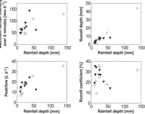
18 events were split at random between a set of 9 events for calibration and a set of 9 events for validation. Rainfall depth P ranged between 10.0 and 139.2 mm, runo_ff depthS between 1.5 and 44.0 mm, maximum rainfall intensity over 5 minPx5between 45.6 and 144.0 mm h−1, peakflowQxbetween 6.8 and 35.7 L s−1, and runoffcoefficient

S/P between 9.3% and 36.0%. Figure 4 presents these last four variables as a

func-5

tion of rainfall depth. Globally, the higher the rainfall depth, the higher the maximum rainfall intensity over 5 min, the higher the runoffdepth, and the higher the peakflow.

3.4 Model parameterization for application on the study site

3.4.1 Input data

To relate rainfall to runoff at the plot scale, the hydrological time series of rainfall and

10

runoff were synchronised on a 1 min time step. Thus, in the model application, the computing interval was 1 min. Concerning input data relative to banana plot geometry, see Sect. 2.1.2.3. Concerning the three modelling approaches, the parameterization is detailed on Table 3. For NoStem,Kswas calibrated. For Stem(1),βwas set to 5% (this value was chosen from preliminary simulations) andKs was calibrated. For Stem(2),

15

Kswas set to 75 mm h−1in accordance with the mean ofKsmeasurements in the field by Cattan et al. (2006).

3.4.2 Analysis of the indicators of the results

To characterize low flows corresponding to recession periods, we defined a Nash and Sutcliffe coefficientNS for measured discharges lower than 5 L s−1, called NS_<₅_i and

20

NS<5for one andNevents, respectively (see Eqs. 31 and 32). In fact,NSon the whole hydrograph favours simulation of the highest discharges at the expense of a good fit of low discharges. WithNS_<₅and NS_<₅_i criteria, we wish to better characterize the role of the stemflow function on the simulation of low flows. We appliedNS<5 and NS<5i

on a period when runoffwas the least influenced by the initial conditions of the soil,

(20)

HESSD

6, 4307–4347, 2009

Title Page

Tables Figures

◭ ◮

Back Close

Full Screen / Esc

i.e. on the recession period (generally occurring after the peak of rainfall) when the soil remained saturated.

To test the hypothesis that the incident rainfall concentration at the plant foot from stemflow generated runofffor rainfall intensities lower thanKs, we compared maximal rainfall intensities Px with calibrated Ks for the three modelling approaches. In the

5

case study, the computing interval of 1 min was considered as unstable relative to measurement uncertainties. To smoothPx for 1 min, maximum rainfall intensities for 5 min,Px₅, were used. Consequently, simulation results are presented as a function of thePx5/Ksratio, which is an adapted indicator of rainfall intensity during a flood event at the plot scale.

10

3.4.3 Calibration procedure

A collective calibration procedure was carried out manually on a set of nine events noted 1 to 9. This calibration was identical for the three approaches, NoStem, Stem(1), and Stem(2). It involved two steps: i) a calibration was performed to obtain a minimal value of the relative errorεS on the simulated runoffdepth (calibration parametersKs 15

orβ according to the approaches – see Table 1), and then ii) an optimisation of the shape of the hydrograph was done to obtain a maximal value ofNScriteria (calibration parametersωandz). With this kind of calibration, the second step cannot influenceεS

criteria, whereas the first step may slightly influenceNScriteria, which are partly linked to the simulated runoffdepth.

20

(21)

HESSD

6, 4307–4347, 2009

Title Page

Tables Figures

◭ ◮

Back Close

Full Screen / Esc

4 Model behaviour and parameter variability

To improve the understanding of stemflow production, we present in this section results of rainfall-runoffsimulations on two events. First, simulations on an event with low and large rainfall intensities were chosen to illustrate the model behaviour according to the three modelling approaches NoStem, Stem(1), and Stem(2). Second, the sensitivity of

5

runoffproduction toKsandβwas determined on a mean rainfall event to illustrate the variability of the parameters described theoretically above.

4.1 Illustration of the model behaviour

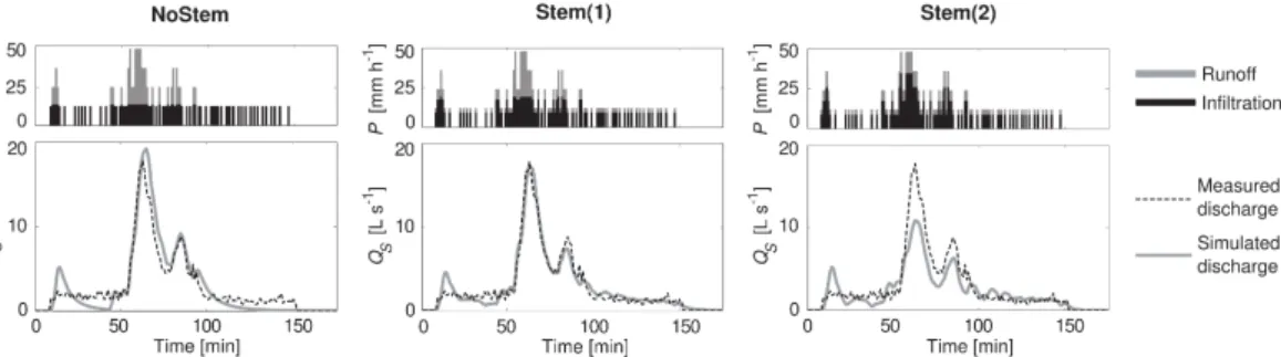
To illustrate the model behaviour, Fig. 5 shows simulations on event 7 for the three approaches, NoStem, Stem(1), and Stem(2). This event was selected because it

pre-10

sented long periods with rainfall intensities lower than the mean Ks value. In Fig. 5 two long periods of residual rainfall appear before and after the rainfall peak, during which rainfall intensities were about 12 mm h−1 and systematically inferior to the Ks

calibration value (i.e. a minimum of 13 mm h−1for NoStem approach).

Figure 5 shows that during this period of residual rainfall (time>100 min), the

No-15

Stem modelling approach did not simulate runoff. Conversely, approaches Stem(1) and Stem(2) simulated a continuous discharge of about 2.5 L s−1. In addition, we ob-served that for Stem(2), runoffvolumes were under-estimated for peakflows. In fact, for high rainfall intensities there was no possible calibration ofβ(first case of the pre-vious theoretical analysis – see Sect. 2.4). In this case, runoffvolume was thus strictly

20

determined by the fixedKsvalue of 75 mm h−1.

4.2 Sensitivity analysis on a representative event

To illustrate the model behaviour described theoretically above, we present a sensitivity analysis on a representative event. We have assumed that a sensitivity analysis carried out on a mean flood event was an indicator of the sensitivity of the model parameters

(22)

HESSD

6, 4307–4347, 2009

Title Page

Tables Figures

◭ ◮

Back Close

Full Screen / Esc

on the other events. This analysis was carried out for event 16 on the four parameters

Ks,β,ω, andz. This event was selected because its rainfall depthP (27.8 mm) and its maximal rainfall intensity over 5 minPx5(76.8 mm h−1) corresponded to the averageP and averagePx5 of the 18 events (Table 2). Calibration using the Stem(1) approach led to the following optimal parameter values:Ks=51.5 mm h−1,β=0.05,ω=7 min, and

5

z=0.47.

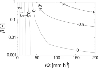
Regarding the sensitivity of runoffproduction to Ks and β, an interaction between these parameters generated an equifinality on runoffdepth calibration because of their impacts on the rainfall-runoff partition at the soil surface. For this reason we wanted to identify the more sensitive calibration parameter,Ks orβ? Figure 6 represents, on

10

a semi-log scale,εSi iso-values according toKsandβ. For a perfect fit of runoffdepth

(i.e.ε_Si=0), the higher theKs, the lower theβ.Ksvalue for aβclose to 1 corresponds to the calibration value for approach NoStem, i.e. 39 mm h−1. Below thisKsthreshold, variations of β cannot o_ffset the insu_fficient infiltration, and consequently the model overestimates the runoff depth. The shape of the curve for ε_Si=0 shows that for Ks 15

values increasing from 39 to 200 mm h−1, which correspond to the range ofKsvalues measured on the field,βdecreases from 1 (equivalent to a model without stemflow, i.e. NoStem approach) to 0.0002. This means that the model is more sensitive toβthan toKs. Finally, if we wish to have only one calibration parameter for runoffsimulations,

βshould be selected rather thanKs.

20

Regarding the sensitivity of hydrographs toωandz, parameter variability of the dif-fuse wave equation has been largely investigated (e.g. Moussa and Bocquillon, 1996; Yu et al., 2000; Chahinian et al., 2006; Tiemeyer et al., 2007). Our results agreed with literature values and confirmed that the higher theωand thez, the lower theQx and the transfer velocity.

(23)

HESSD

6, 4307–4347, 2009

Title Page

Tables Figures

◭ ◮

Back Close

Full Screen / Esc

5 Comparison of modelling approaches “without” and “with” stemflow

5.1 Global analysis of calibration and validation sets

5.1.1 Calibration results

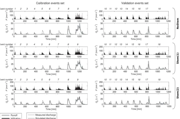
Simulations of the calibration set carried out to optimise the runoff volume (εS=0)

showed that the shape of the simulated hydrograph was better simulated with the

stem-5

flow function than without (Table 3): for the calibration set,NSwas 0.69, 0.88, and 0.92 for NoStem, Stem(1), and Stem(2), respectively. To assess the model performances on all events, a split-sample test (Klemeˇs, 1986) was conducted. This test considers that each set of events (event numbers 1 to 9 and 10 to 18 in our case study – Table 2) should be used in turn for calibration and validation. Taking events 10 to 18 for

calibra-10

tion and 1 to 9 for validation led to similarNSvalues for calibration, that is to say 0.61, 0.80, and 0.82 for the same three approaches, respectively.

Regarding performance criteria of peakflows (ε_Qx) in Table 3 for the calibration set, peakflows were overestimated for all approaches but were better simulated with the stemflow function (ε_Qx0.36, 0.18, down to 0.02 for NoStem, Stem(1), and Stem(2),

re-15

spectively). But with poorer results, low flows were unequally simulated (NS_<5−0.55, 0.35, up to 0.47 for NoStem, Stem(1), and Stem(2), respectively). Finally, these results showed that the modelling approach with stemflow globally improved model perfor-mances.

Moreover, the model with stemflow adequately simulated runo_ff volumes, with

20

a meanKs value equal to the mean of field measurements (75 mm h−1): for NoStem, calibrated Ks was 44.4 mm h−1, whereas for Stem(1), Ks was higher (60.5 mm h−1). Additionally, we noticed that the lag timeω decreased by nearly half when using the stemflow function, with values of 16, 11, and 9 min for approaches NoStem, Stem(1), and Stem(2), respectively. This decrease in response time indicates that the

trans-25

(24)

HESSD

6, 4307–4347, 2009

Title Page

Tables Figures

◭ ◮

Back Close

Full Screen / Esc

and thus to simulating runofffor residual rainfall in the recession period, although the production function did not produce runo_ffduring this period. Conversely, approaches Stem(1) and Stem(2) produced runofffor residual rainfall in the recession period. Con-sequently, good simulations were obtained with faster transfer. Finally, the shape pa-rameterz varied little from an approach to another, and was about 0.48.

5

5.1.2 Validation results

Globally, the three approaches simulated runoffvolumes well on the validation set with

ε_S values inferior to 0.17. As seen for calibration results, modelling approaches with stemflow improved simulation of flood hydrographs for validation sets (Table 3): NS

was 0.53, 0.75, and 0.81 for NoStem, Stem(1), and Stem(2), respectively, and was

10

0.61, 0.89, and 0.90 for the split-sample test detailed above. However, contrary to the calibration results, the other performance criteria of peak and low flows were poorly simulated for the three approaches withε_Qx values superior to 0.45, and with negative

NS_<5values (Table 3). To better understand the disparity of the simulation results of the calibration and validation sets, the next section will analyse the model performances

15

event by event.

5.2 Event by event analysis

Performance criteria of the model simulations event by event – shown in Fig. 7 – are plotted in Fig. 8 as a function ofPx₅/Ks, which represents the ratio between the maxi-mal rainfall intensity over 5 min and the saturated hydraulic conductivity.

20

Regarding the criteria on runoffvolume, NoStem shows an increasing function ofε_Si

vs.Px₅/Ks, leading to an under-estimation of the lowest rainfall events and an over-estimation of the highest. This ε_Si vs.Px5/Ks relationship became less marked for Stem(1) and disappeared for Stem(2), meaning that the stemflow function improved the simulation of runo_ffvolume for all events, notably with low rainfall intensities. The

25

(25)

HESSD

6, 4307–4347, 2009

Title Page

Tables Figures

◭ ◮

Back Close

Full Screen / Esc

is also better with stemflow.

Concerning the simulation of the hydrograph, modelling with a stemflow function im-proved the shape of the whole hydrograph as well as the shape of low flows, especially for low rainfall intensities. In fact, the number of events out of 12 withPx5/Ks<1 having

NS_i andNS_<₅_i values superior to 0.8 were 0 and 0 for NoStem, 7 and 6 for Stem(1),

5

and 7 and 4 for Stem(2), respectively.

Finally, NoStem, Stem(1), and Stem(2) gave good performances for events having aPx₅/Ksclose to 1 (in other words for which the maximum rainfall intensity was close to the calibratedKs value; events 6, 14, 15, and 16 in Fig. 7). And the Stem(1) and Stem(2) approaches considerably improved runoffmodelling for rainfall events with low

10

intensities, notably those lower than the measuredKs. On the other hand, these results showed thatβcan be an efficient calibration parameter whenKsis measured in situ.

6 Discussion and conclusion

Our results show that taking into account the rainfall partitioning by vegetation in a runoff model improved discharge simulation at the plot scale, in the case of a

ba-15

nana field. This approach was consistent with the high permeability values measured on the field and accounts for the production of runo_fffor rainfall intensities lower than surface saturated hydraulic conductivity. This modelling approach was lumped at the plot scale, in which we developed a stemflow function that was coupled with a produc-tion funcproduc-tion and a transfer funcproduc-tion. The applicaproduc-tion on a banana field under tropical

20

rainfalls in Guadeloupe gave good results (NS_i>0.6 for 14 events out of 18) for a wide range of rainfall events from 10 to 130 mm depth. This last point highlights the robust-ness of the model and allows it to be considered for application on long time series.

Our study showed the influence of plant canopy on hydrological processes at the 3000 m2plot scale. Simulations showed that the rainfall concentration at the plant foot

25

(26)

HESSD

6, 4307–4347, 2009

Title Page

Tables Figures

◭ ◮

Back Close

Full Screen / Esc

rainfall intensities. Concerning low flows, although results without and with stemflow showed that it was difficult to simulate runoffduring low rainfalls, low flows were better modelled with stemflow. This result is coherent with the decrease inKsobserved at the end of the rainfall event by Cattan et al. (2009) at the banana plant scale. In fact, this decrease in permeability generates more runoffand is equivalent to a concentration of

5

rainwater at the soil surface in our modelling approach with stemflow.

One limitation of the modelling approach lies in the concept of the hydraulic compart-mentation of the plot, with one compartment receiving a water pathway from stemflow. In fact, the physical measurement of the stemflow coefficientβ, which determines the area of both compartments, may be difficult because the boundaries of the water

path-10

ways vary in space and time as shown by Cattan et al. (2009). Thus, this conceptual two-compartment scheme implies that the parameter of the stemflow function should remain calibrated.

The major implication of this study concerns the management of water fluxes in a cultivated plot. First, our study shows that, to account for rainfall partitioning

be-15

tween runoff and infiltration, changes in the structure and arrangement of cropping species should be considered as well as the more traditional soil management tech-niques (plant cover, mulching, soil tillage ...). Second, the structure and arrangement of cropping species should be taking into account to globally manage transfers in and out of the plot. Indeed, the great heterogeneity of water fluxes at the soil surface that

20

are induced by plant cover may influence transport of solute elements (fertilizers and pesticides) or solid elements (erosion). Some authors have shown the role of banana stemflow in drainage water on transport of nitrate and potassium (Sansoulet et al., 2007) and of pesticides (Saison et al., 2008), confirming the need to consider these processes. This is especially true since applications of agrochemicals on banana fields

25

are not spatially distributed over the whole area: in the case of banana, applications are localized around the plant collar, i.e. in zones of high water fluxes from stemflow.

(27)

HESSD

6, 4307–4347, 2009

Title Page

Tables Figures

◭ ◮

Back Close

Full Screen / Esc

of long duration with relatively low intensities, situations for which authors like Yu et al. (2000) and Chahinian et al. (2006) have noted the modelling di_fficulties. Finally, consid-ering the influence of vegetation on runoffgeneration at the plant and the plot scales, its influence on hydrological processes at a larger scale, that of the hillslope and the catchment scales, have to be assessed. The proposed stemflow function integrated

5

into a lumped model at the plot scale can be used in distributed hydrological models at the catchment scale to characterize vegetation impact on hydrological processes.

Acknowledgement. This study was funded by the Guadeloupe Region (FWI), the Minist `ere

de l’Ecologie et du D ´eveloppment Durable (France), and the European Community under the project “Assessment of water-pollution risks associated with agriculture in the French West

10

Indies: management at the catchment scale”.

References

Ajayi, A. E., Van de Giesen, N., and Vlek, P.: A numerical model for simulating Hortonian overland flow on tropical hillslopes with vegetation elements, Hydrol. Process., 22(8), 1107– 1118, 2008.

15

Belk, E. L., Markewitz, D., Rasmussen, T. C., Carvalho, E. J. M., Nepstad, D. C., and Davidson, E. A.: Modeling the effects of throughfall reduction on soil water content in a Brazilian Oxisol under a moist tropical forest, Water Resour. Res., 43, W08432, doi:10.1029/2006WR005493, 2007.

Bouten, W., Schaap, M. G., Bakker, D. J., and Verstraten, J. M.: Modelling soil water dynamics

20

in a forested ecosystem. I: A site specific evaluation, Hydrol. Process., 6(4), 435–444, 1992. Cattan, P., Cabidoche, Y.-M., Lacas, J.-G., and Voltz, M.: Effects of tillage and mulching on

runo_ffunder banana (Musaspp.) on a tropical Andosol, Soil Till. Res., 86(1), 38–51, 2006. Cattan, P., Bussi `ere, F., and Nouvellon, A.: Evidence of large rainfall partitioning patterns by

ba-nana and impact on surface runoffgeneration, Hydrol. Process., 21(16), 2196–2205, 2007a.

25

(28)

HESSD

6, 4307–4347, 2009

Title Page

Tables Figures

◭ ◮

Back Close

Full Screen / Esc

Cattan, P., Ruy, S., Cabidoche, Y.-M., Findeling, A., Desbois, P., and Charlier, J.-B.: Effect on runoffof rainfall redistribution by the impluvium-shaped canopy of banana cultivated on an Andosol with a high infiltration rate, J. Hydrol., 368(1–4), 251–261, 2009.

Chahinian, N., Moussa, R., Andrieux, P., and Voltz, M.: Accounting for temporal variation in soil hydrological properties when simulating surface runoff on tilled plots, J. Hydrol., 326(1–4),

5

135–152, 2006.

Charlier, J.-B.: Fonctionnement et mod élisation hydrologique d’un petit bassin versant cultiv é en milieu volcanique tropical, PhD thesis, Universit é des Sciences et Techniques du Langue-doc, Montpellier II, 246 pp., 2007.

Crockford, R. H. and Richardson, D. P.: Partitioning of rainfall into throughfall, stemflow and

10

interception: effect of forest type, ground cover and climate, Hydrol. Process., 14(16–17), 2903–2920, 2000.

Gash, J. H. C., Lloyd, C. R., and Lachaud, G.: Estimating sparse forest rainfall interception with an analytical model, J. Hydrol., 170(1–4), 79–86, 1995.

Green, W. A. and Ampt, G. A.: Studies on soil physics, 1: The flow of air and water through

15

soils, J. Agr. Sci., 4(1), 1–24, 1911.

Harris, D.: The partitioning of rainfall by a banana canopy in St Lucia, Windward Islands, Trop. Agr., 74, 198–202, 1997.

Hayami, S.: On the propagation of flood waves, Disaster Prev. Res. Inst. Bull., Kyoto University, 1, 1–16, 1951.

20

Herwitz, S. R.: Infiltration-excess caused by Stemflow in a cyclone-prone tropical rainforest, Earth Surf. Proc. Land., 11(4), 401–412, 1986.

Horton, R. E.: The role of infiltration in the hydrologic cycle, EOS T. Am. Geophys. Un., 14, 446–460, 1933.

Keim, R. F. and Skaugset, A. E.: A linear system model of dynamic throughfall rates beneath

25

forest canopies, Water Resour. Res., 40(05), W05208, 2004.

Klemeˇs, V.: Operational testing of hydrological simulation models, Hydrol. Sci. J., 31(1), 13–24, 1986.

Levia, D. F. J. and Frost, E. E.: A review and evaluation of stemflow literature in the hydrologic and biogeochemical cycles of forested and agricultural ecosystems, J. Hydrol., 274, 1–29,

30

2003.

(29)

HESSD

6, 4307–4347, 2009

Title Page

Tables Figures

◭ ◮

Back Close

Full Screen / Esc

Llorens, P. and Domingo, F.: Rainfall partitioning by vegetation under Mediterranean conditions. A review of studies in Europe, J. Hydrol., 335, 37–54, 2007.

M ´et ´eo-France: http://www.meteofrance.com/, 2004.

Morel-Seytoux, H. J.: Derivation of equations for variable rainfall infiltration, Water Resour. Res., 14(4), 561–568, 1978.

5

Moussa, R. and Bocquillon, C.: Algorithms for solving the diffusive wave flood routing equation, Hydrol. Process., 10(1), 105–123, 1996.

Moussa, R., Voltz, M., and Andrieux, P.: Effects of the spatial organization of agricultural man-agement on the hydrological behaviour of a farmed catchment during flood events, Hydrol. Process., 16(2), 393–412, 2002.

10

Philip, J. R.: The theory of infiltration: 4. Sorptivity and algebraic infiltration equations, Soil Sci., 84, 257–267, 1957.

Richards, L. A.: Capillary conduction of liquids through porous medium, Physics, 1(5), 318– 333, 1931.

Saison, C., Cattan, P., Louchart, X., and Voltz, M.: Effect of spatial heterogeneities of water

15

fluxes and application pattern on cadusafos fate on banana-cultivated andosols, J. Agr. Food Chem., 56(24), 11947–11955, 2008.

Sansoulet, J., Cabidoche, Y. M., and Cattan, P.: Adsorption and transport of nitrate and potas-sium in an Andosol under banana (Guadeloupe, French West Indies), Eur. J. Soil Sci., 58(2), 478–489, 2007.

20

Sansoulet, J., Cabidoche, Y.-M., Cattan, P., Ruy, S., and ˇSim ˘unek, J.: Spatially distributed water fluxes in an andisol under banana plants: Experiments and three-dimensional modeling, Vadose Zone J., 7(2), 819–829, 2008.

Singh, V. P.: Accuracy of kinematic wave and diffusion wave approximations for space indepen-dent flows, Hydrol. Process., 8(1), 45–62, 1994.

25

Tiemeyer, B., Moussa, R., Lennartz, B., and Voltz, M.: MHYDAS-DRAIN: A spatially distributed model for small, artificially drained lowland catchments, Ecol. Model., 209(1), 2–20, 2007. Van Dijk, A. I. J. M. and Bruijnzeel, L. A.: Modelling rainfall interception by vegetation of variable

density using an adapted analytical model. Part 1. Model description, J. Hydrol., 247(3–4), 230–238, 2001.

30

(30)