Modeling Air Bubble Transport in Hydraulic Jump Flows using Population Balance Approach

Journal of Applied Fluid Mechanics, Vol. 9, No. 2, pp. 965-973, 2016. Available online at www.jafmonline.net, ISSN 1735-3572, EISSN 1735-3645.

Modeling Air Bubble Transport in Hydraulic Jump Flows

using Population Balance Approach

M. Xiang

and J. Y. Tu

1. _{Institute of Aerospace and Material Engineering, National University of Defense Technology, Changsha} 410073, P.R. China

2. _{School of Aerospace, Mechanical and Manufacturing Engineering, RMIT University, Victoria 3083,} Australia

†Corresponding Author Email: xiangmin333@hotmail.com

(Received March 21, 2014; accepted March 16, 2015)

A

This paper proposed a numerical model aiming at coupling the MUltiple-SIze-Group (MUSIG) with the semi-empirical air entrainment model based on the Euler-Euler two-fluid framework to handle the bubble transport in hydraulic jump flows. The internal flow structure including the recirculation region, the shear layer region and the jet region was accurately predicted. The flow parameters such as the water velocity and void fraction distributions were examined and compared with the experimental data, validating the effectiveness of the numerical model. Prediction of the Sauter mean bubble diameter distributions by the population balance approach at different axial locations confirmed the dominance of breakage due to the high turbulent intensity in the shear layer region which led to the generation of small gas bubbles at high void fraction. Comparison between different cases indicates that high Froude number not only give rise to longer recirculation region and higher void fraction due to larger air entrainment rate, but also generate larger bubble number density and smaller bubble size because of the stronger turbulence intensity in the same axial position.

Keyword: Hydraulic jump; Air entrainment; Bubbly flow; MUSIG.

N

BB birth rate due to breakage Bc birth rate due to coalescense C k~ turbulence model constant

Cb bubble induced turbulent viscosity constant d1 the water depth immediately upstream of the

jump toe

d2 the water depth downstream the jump D diameter

DB death rate due to breakage Dc death rate due to coalescense Ds sauter mean bubble diameter Fi total interfacial force Fr onset Froude number Fre onset Froude number g gravitational acceleration h height of vertical gate

Subscripts

a air g gas

i index of gas/liquid phase j index of gas/liquid phase

k turbulent kinetic energy K1 adjustable constant

ni average number density of the ith class P pressure

Q volumetric rate u velocity u velocity vector

ue onset velocity for gas entrainment

 void fraction

 turbulent kinetic energy dissipation rate

 molecular viscosity

t,b bubble induced turbulent viscosity

e

effective viscosity

 density

k index of gas/liquid phase l liquid

1.

I

Hydraulic jump is a natural flow characteristic which is frequently encountered in many hydraulic structures, industrial open channels and manufacturing processes. In general, a hydraulic jump involves complex flow energy dissipation and transition from supercritical to subcritical flow region; resulting in a sudden velocity reduction and increment in depth in flow direction. Complex multiscale phenomena are involved in the hydraulic jump flow as shown in Fig. 1. Large scale turbulent free-surface is formed along the main flow propagating direction. At the jump toe, significant amount of air are entrapped caused by the strong interaction between turbulence and free surface, giving birth to numerous poly dispersed bubbles. Two distinguished regions are generated downstream of the entrainment point (Chachereau and Chanson, 2011): in the recirculation region, rigorous kinetic energy dissipation occurs in the form of turbulent rollers; In the shear layer region, the entrapped air bubbles are advected forming a bubbly two-phase flow downstream. The resultant distributions of void fraction, bubble number density and bubble sizes have strong implications in terms of air-water mixing and mass transfer processes. Theoretically speaking, the aforementioned flow structures are extremely complex and closely coupled physical phenomena occurring in multiple forms of fluids (e.g. continuum air, continuum water and dispersed air bubbles). The underlying physics of these phenomena remain largely elusive.

Fig. 1. Schematic of air entrainment for hydraulic jump flows.

During the last decade, numerous experimental works has been conducted to examine in details the air-water flow properties in hydraulic jumps, among which the most outstanding work was carried out by the group of Chanson, covering various aspects of hydraulic jump flows. The experiments were implemented in a wide range of Froude numbers by (Chanson, 2009; Chanson, 2010; Murzyn and Chanson, 2007) to explore the upstream flow condition effect. Detail measurement of the large-scale flow properties including the free-surface location and the fluctuations, the micro-scale

two-phase properties such as the vertical void fraction, velocity and bubble frequency profiles in different regions, as well as the turbulence characteristics by (Chanson, 2007) were given. Then the systematic study of dynamic similarity and scale effects for hydraulic jump flow was carried out (Chanson, 2006), implying significant scale effect for the hydraulic jump flows. These experimental works gave primary insight on the complex phenomena imbedded in the hydraulic jump flows. However, characteristic of the internal flow phenomena including turbulence, air bubble entrainment and interactions between entrained bubbles and coherent structures needs to be better understood.

Considering the expense of experimental technique and the scale effects, CFD tools are required to be applied for the simulation of hydraulic structures. Nevertheless, the complexity of air entrainment and bubble evolution processes pose a great challenge for the model development. Recently, several researchers (Ma and Hou, 2001; Passandideh-Fard et al., 2007; Sabbagh-Yazdi SR, 2007) attempted to capture the large-scale free-surface properties using free surface capture models (VOF and Level Set). However, the air void fraction distributions were not predicted because the two-phase nature of the flow and the associated air entrainment were ignored. In order to model the air entrainment rate, several numerical models have been proposed to consider various air entrainment mechanisms. Skartlien et al. (2012) developed a simplified physical model for air entrainment in the hydraulic jump, considering different air entrainment mechanisms. Waltz (2008) incorporated the air entrainment at the free surface into the two-phase flow models based on the commercial code FLOW-3D. The void fraction, velocity and turbulence dissipation rate distribution were compared with experimental data. Cheng and Chen (2011) proposed an improved drag model to consider both the free surface and the gas bubbles, predicting the air void fraction distributions and velocity profiles suitable. Ma et.al (2011) obtained the first accurate, quantitative numerical prediction of the overall void fraction distributions in a hydraulic jump using the sub-grid air entrainment model coupled with the two-fluid model. Nevertheless, the previous research have not presented the bubble size evolution process, which is however critical for the air-water mass transfer properties.

explicitly through fundamental interfacial momentum transfer models. The MUltiple-SIze-Group (MUSIG) model (Cheung et al., 2007; Xiang et al., 2011) together with mechanistic coalescence and breakage kernels are also coupled in the model to better represent the air bubble size evolution in the subcritical flow region. Numerical predictions are validated against the recent experimental work carried out by Chachereau and Chanson (2011).

2. M

2.1 Semi-Empirical Air Entrainment Model

for Hydraulic Jump

Due to the complexity of the bubble entrainment process and lack of knowledge on the bubble entrainment mechanism, it is difficult to establish accurate air entrainment model. In this study, the theoretical model proposed by Wood (1991) was adopted by connecting the air entrainment model with the upstream velocity V1.

2 1 1 1 ( ) a e l

Q V V

K

Q gd





where Ve is the onset velocity of air entrainment for hydraulic jump flow which is calculated by the onset Froude number Fr_eV_e/ gd₁1. d1 is the water depth immediately upstream of the jump toe and K1 is an adjustable constant. This equation implies that air entrainment rate increases with Froude number.

2.2 Two-Fluid Model

The two-fluid model based on the Eulerian– Eulerian framework solves the ensemble-averaged of mass, momentum and energy whereby the liquid is considered as the continuum phase and the gas is treated as disperse phase. Two sets of governing equations are solved for each phase. Interactions between phases are effected via interfacial transfer terms for heat, mass and momentum exchange. Since there is no interfacial mass or heat transfer between the phases in the present study, the energy equation is not needed to be solved.

In the absence of interfacial mass transfer, the continuity equation of the two-phases can be written as:

( )

( ) 0

i i

i i i

t

  _{ }

 _{   }

 u

where ,  and u are the void fraction, density and velocity vector of each phase. Subscripts i = l or g denote the liquid and gas phase respectively. The momentum equation can be expressed as:

T T ref ( ) ( ) [ ( ( ) )] ( )

i i i

i i i i i

e

i i i i i i

i i P t             _{       }           u u u

g u u

g F

(3)

where l is adopted as the reference density ref to calculate the buoyancy force. Fi represents the interfacial forces for the interfacial momentum transfer and g is the gravity acceleration vector. It is noted that the interfacial forces appearing in the momentum equation strongly govern the distribution of the liquid and gas phases within the flow volume. Details of the different forces acting within the two-phase flow can be found in our previous work (Xiang et al., 2011).

2.3 Population Balance Model

The population balance method is adopted to predict the size distribution of the poly-dispersed bubbles. The analysis is simplified by considering bubble sizes change due to breakup and coalescence events only, i.e. nucleation, growth and/or dissolution of bubbles due to absorption (desorption) or boiling, does not occur. The population balance equation is solved with application of the MUSIG model which employs multiple discrete bubble size groups to represent the population balance of bubbles. Assuming each bubble class travel at the same mean algebraic velocity, individual number density of bubble class i can be expressed as (Kumar and Ramkrishna, 1996):

C B C B

( )

i

g i

n

u n B B D D

t

 _{      }

  (4)

where ni is the average bubble number density of the ith group, the source terms BC, BB, DC and DB are, respectively, the birth rates due to coalescence and break-up and the death rate due coalescence and break-up of bubbles. The break-up rate of bubbles is computed according to the model developed by Luo and Svendsen (1996), which is developed based on the assumption of bubble binary break-up under isotropic turbulence situation. Bubble coalescence may be caused by wake entrainment, random turbulence and buoyancy. However, as all bubbles travel at the same velocity in the MUSIG model, buoyancy effect is eliminated. The coalescence rate considering only turbulent collision is taken from Prince and Blanch (1990).

2.4 Turbulence Model

viscosity of the liquid phase is considered as being composed of the molecular viscosity l , the turbulent viscosity t,l and the bubble induced turbulent viscosity t,b:

, ,

e

l l t l t b

    (5)

Two-equation k- model is applied to determine the liquid turbulent viscosity:

2 ,

t l l

k C

 



 (6)

where the turbulent kinetic energy k and its dissipation rate  in Eq. (6) of the continuous liquid phase are determined from transport equations which are straightforward extensions of the standard k- model(Lopez De Bertodano et al., 1994). Effect of turbulent in the liquid phase on turbulence in the gas phase may be modeled by setting the viscosity to be proportional to the liquid turbulent viscosity:

g e e g l l    

 (7)

The extra bubble induced turbulent viscosity in Eq. (5) is evaluated according to the model by Sato et

al.(1981):

,

t b lCb gD us g ul

     with C_b0.6 (8)

3. E

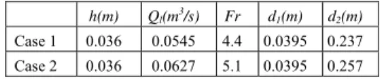
The experiments carried out in a 3.2m×0.5m×0.45m horizontal rectangular tunnel by Chachereau and Chanson (Chachereau and Chanson, 2011) were used for investigation. The experiments were performed with inflow Froude numbers between 2.4 and 5.1 which were corresponding to Reynolds numbers between 6.6×104 and 1.3×105. The inflow condition was controlled by a vertical gate which was fixed at height h of 0.036m during all experiments. Detailed air-water flow measurements at the sub-millimetric scale were conducted using the double-tip conductivity probe. Two cases with different Froude number as shown in Table 1 were selected for investigation, where Ql is water flow rate and Fr is the Froude number calculated by upstream water velocity and flow depth. d2 is the flow depth

Table 1 Experimental cases description

h(m) Ql(m 3

/s) Fr d1(m) d2(m)

Case 1 0.036 0.0545 4.4 0.0395 0.237

Case 2 0.036 0.0627 5.1 0.0395 0.257

Considering that the experimental data used for investigation were all time-averaged values, steady simulations were carried out, aiming at exploring the time-averaged two-phase flow characteristics. Numerical simulations were performed on a two-dimensional computational domain. The free surface profile of the hydraulic jump which was assumed to remain steady and stationary in computational domain was evaluated according to the experimental measurement. The bubbles were entrained through a source point located at the hydraulic jump toe. The free surface was set as a degassing boundary where the dispersed bubbles are permitted to escape and the liquid is free slipping. The bottom wall was modeled as no-slip for both liquid and gas phases. A bubble diameter of 1.5 mm was used for the initial entrained bubble size in the simulation, which was estimated from the mean bubble diameter reported in the experiment (Chachereau and Chanson, 2011). Based on sensitivity tests on bubble group numbers, we adopted 10 groups by equal splitting in the range of 0mm and 10mm.The computational domain was discretized into 16100 non-uniform cells with a minimum spacing of 0.002m in x direction. The generic CFD code ANSYS CFX12 was utilized as the basic simulation platform. The transport equations of the two-fluid and population balance models were discretized by the finite volume approach. The convection terms were approximated by a high order resolution scheme while the diffusion terms were approximated by the second-order central difference scheme. A fixed physical time scale of 0.001 s was adopted to achieve steady state solutions. Convergence was achieved within 5000 iterations when the RMS (root mean square) residual dropped below 10-5.

4. R

4.1 Flow Structure Analysis

(a) Case 1

(b) Case 2

Fig. 2. Streamlines of liquid.

Fig. 3 presents the gas void fraction distributions generated by air entrainment. The gas bubbles being entrained were seen to follow closely with the streamlines of the vortex within the recirculation region. Hence, the residence time of the gas bubbles in this region increased as the region was more populated by the gas bubbles. Due to the buoyancy force, bubbles tended to migrate to the free surface, giving rise to much higher void fraction in the upper vortex region. Downstream of the recirculation region, most of the bubbles were floated up and dispersed away along the free surface.

Fig. 4 compares the predicted dimensionless water velocity profiles with the experimental data for Case 1. x refers to the axial distance from the jump toe and u1 refers to the velocity upstream the jump toe. Due to the affection of wall shear stress, the liquid velocity gradually increased from the bottom until reaching the maximum value at the boundary of the jet region. Thereafter high negative velocity gradient was observed in the shear layer region induced by strong momentum transfer between the jet region and the recirculation region. Subsequently, the liquid velocity gradually decreased to negative values, indicating that the flow started to recirculate. Along with the flow developing away from the entrainment point, the maximum velocity point moved closer to the bottom wall which was resulted from the expanding of the shear layer region. However, the momentum transfer between the jet region and recirculation

region was gradually weakened illustrated by the flat velocity profile. The predicted water velocity agrees well with the experimental data, validating that the flow structure was successfully captured.

(a) Case 1

(b) Case 2

Fig. 3. Contours of gas void fraction.

4.2 Polydispersed Bubble Distributions

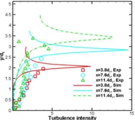
in the high void fraction region maybe under-predicted. Compared with Case 1, higher void fraction was observed in the same axial section for Case 2 due to larger air entrainment rate under higher Froude number. High turbulence and strong variation of void fraction will induce severe coalescence and breakup between bubbles.

(a) x/d1=3.8 (b) x/d1=7.6

(c) x/d1=11.4 (d) x/d1=18

Fig. 4. Comparison of dimensionless water velocity profile corresponding at different axial positions downstream gas entrainment point for Case 1 with

experimental data.

Fig. 6 gives the bubble number density distributions corresponding at different axial sections. In accordance with the void fraction distribution, low number density was observed in the jet region while in the shear layer region the bubble number increased rapidly to the maximum value. However, the maximum number density point appeared closer to the bottom surface then the former characteristic point. This is because high void fraction enhances bubble coalescence which reduces the bubble number. Subsequently, the bubble number density which follows the void fraction curve decreased rapidly as the bubbles dispersing into the upper

recirculation region. However, in the near free surface region, an extremely low value was observed for the number density which was in contrary to the void fraction distributions, indicating most of the bubbles were merged into large ones due to high coalescence rate. With the distance increasing from the entrainment point, the maximum number density decreased remarkably. In comparison with the measured bubble count rate (Chachereau and Chanson, 2011), the variation trend of bubble number density agrees well with the experimental data. Compared with Case 1, the maximum bubble number density for Case 2 was bigger in the same axial section due to the larger air entrainment rate and the higher jet velocity which gave rise to higher breakup rate.

(a) Case 1

(b) Case 2

Fig. 5. Radial void fraction distribution corresponding at different axial positions.

void fraction was also increasing dramatically in this region which resulted in the coalescence of bubbles, the minimum size bubble was formed before the maximum number density point. Thereafter, the coalescence effect dominated, leading to larger bubble sizes and these bubbles were driven by buoyancy to the upper region.

(a) Case 1

(b) Case 2

Fig. 6. Dimensionless bubble number density distributions corresponding at different axial

positions.

The bubble diameter in the maximum bubble number density point represented by dNmax was investigated in Table 2. A slightly decreasing trend was observed for the bubble diameter in this characteristic point due to the decreasing void fraction along the axial direction. However, with the flow developing downstream, the turbulence intensity was weakened as well which enhances the bubble coalescence. The bubble size evolution trend depends on the dominated effect between these two factors. In the same axial position, the average bubble size was smaller for case 2 resulted from the higher jet velocity at the boundary of the shear layer region which was in accordance with the number density distributions. In comparison with the experimental data, the bubble diameter was under predicted.

(a) Case 1

(b) Case 2

Fig. 7. Sauter mean bubble diameter distributions corresponding at different axial

positions.

Table 2 Sauter mean bubble diameter in the characteristic points of the shear layer region

X/D1 3.8 7.6 11.4

Case 1 dNmax,sim 0.58 0.56 0.55 dNmax,Exp 1.28 1.16 1.15 Case 2 dNmax,sim 0.55 0.56 0.53 dNmax,Exp 1.22 1.28 1.05

Fig. 8. Turbulence intensity distributions corresponding at different axial positions for

Case 2.

5. C

A numerical model, which was coupled with the population balance approach and a semi-empirical air entrainment model, has been established to predict the bubble transport in hydraulic jump flow based on the Euler-Euler two-fluid model. Three different regions including the jet flow region, shear layer region and recirculation region were successfully captured. The predicted water velocity and void fraction in different regions agree well with the experimental data, validating that the numerical model is capable of capturing main characteristics of the bubbly flow induced by air entrainment in hydraulic jump flows.

In the shear layer region where both high void fraction and high turbulence intensity exist, two characteristic points including the maximum void fraction point and the maximum bubble number density point were observed. The maximum number density point was closer to the bottom surface than the maximum void fraction point due to the coalescence effect induced by high void fraction. The average bubble diameter at the maximum number density point almost maintain constant along the axial direction due to opposite effect of decreasing void fraction and decreasing turbulence intensity. To our knowledge, this is the first numerical study to explore the bubble size evolution process for hydraulic jump. Further research will focus on establishing multiscale simulation model to obtain more accurate results by coupling the air entrainment with the free surface formation process.

ACKNOWLEDGMENT

The financial support provided by the National Natural Science Foundation of China (Project ID 51406230).

R

Chachereau, Y. and H. Chanson (2011). Free-surface fluctuations and turbulence in hydraulic jumps. Experimental Thermal and Fluid Science 35, 896-909.

Chanson, H. (2006). Air bubble entrainment in hydraulic jumps. Similitude and scale effects. Report NO. CH57/05, Brisbane, Australia, The University of Queensland.

Chanson, H. (2007). Bubbly flow structure in hydraulic jump. European Journal of Mechanics B-Fluids 26, 367-384.

Chanson, H. (2009). Advective diffusion of air bubbles in hydraulic jumps with large Froude numbers:an experimental study. REPORT CH75/09, Brisbane, AUSTRALIA, The University of Queensland.

Chanson, H. (2010). Convective transport of air bubbles in strong hydraulic jumps. International Journal of Multiphase Flow 36, 798-814.

Cheng, X. J. and X. W. Chen (2011). Applying Improved Eulerian Model for Simulation of Air-Water Flow in a Hydraulic Jump. World Environmental and Water Resources Congress.

Cheung, S. C. P., G. H. Yeoh and J. Y. Tu (2007). On the numerical study of isothermal vertical bubbly flow using two population balance approaches. Chemical Engineering Science 62, 4659-4674.

Kumar, S. and D. Ramkrishna (1996). On the solution of population balance equations by discretisation—I. A fixed pivot technique. Chemical Engineering Science 51, 1311-1332.

Lopez De Bertodano, M., J. R. T. Lahey, O. C. Jones and A. Et (1994). Development of a k-ε model for bubbly two-Phase Flow. Journal of Fluids Engineering 116, 128-134.

Luo, H. and H. Svendsen (1996). Theoretical model for drop and bubble breakage in turbulent dispersions. AIChE Journal 42, 1225–1233. Ma, F. and Y. Hou (2001). Numerical calculation of

submerged hydraulic jumps. Journal of hydraulic research 39, 493-503.

Ma, J., A. A. Oberai, R. T. L. Jr and D. A. Drew (2011). Modeling air entrainment and transport in a hydraulic jump using two-fluid RANS and DES turbulence models. Heat Mass Transfer 47, 911-919.

bubbly flow and turbulence measurements in hydraulic jumps. The University of Queensland, Brisbane.

Passandideh-Fard, M., A. R. Teymourtash and M. Khavari (2007). Numerical Study of Circular Hydraulic Jump Using Volume-of-Fluid Method. Journal of Fluids Engineering 133, 1-11.

Prince, M. J. and H. W. Blanch (1990). Bubble coalescence and breakage in air sparged bubble columns. AIChE Journal 36, 1485–1499. Sabbagh-Yazdi, F. R. (2007). Turbulent modeling

effects on finite volume solution of three dimensional aerated hydraulic jumps using volume of fluid. Proceedings of the 12th WSEAS International Conference on Applied Mathematics 168-174.

Sato, Y., M. Sadatomi and K. Sekoguchi (1981). Momentum and heat transfer in two-phase bubbly flow—I. International Journal of Multiphase Flow 7, 167-178.

Skartlien, R., J. A. Julshamn, C. J. Lawrence and L.

Liua (2012). A gas entrainment model for hydraulic jumps in near horizontal pipes. International Journal of Multiphase Flow 43, 39-55.

WALTZ, J. D. (2008). A Study on Internal Flow Features and Air Entrainment Effects in Hydraulic Jumps Using Numerical Modeling Techniques, Universitu of California.

Wood, I. R. (1991). Air entrainment in free-surface flows. Rotterdam, The Netherlands, IAHR Hydraulic Structures Design Manual NO.4, Hydraulic Design Considerations, Balkema Publishers.

Xiang, M., S. C. P. Cheung, G. H. Yeoh, W. H. Zhang and J. Y. Tu (2011). On the numerical study of bubbly flow created by ventilated cavity in vertical pipe. International Journal of Multiphase Flow 37, 756-768.