www.atmos-chem-phys.net/13/10113/2013/ doi:10.5194/acp-13-10113-2013
© Author(s) 2013. CC Attribution 3.0 License.
Atmospheric
Chemistry
and Physics
Stratospheric O
3
changes during 2001–2010: the small role of solar
flux variations in a chemical transport model
S. S. Dhomse1, M. P. Chipperfield1, W. Feng1, W. T. Ball2, Y. C. Unruh2, J. D. Haigh2, N. A. Krivova3, S. K. Solanki3,4, and A. K. Smith5
1School of Earth and Environment, University of Leeds, Leeds, UK
2Physics Department, Blackett Laboratory, Imperial College London, London, UK 3Max-Planck-Institut für Sonnensystemforschung, Katlenburg-Lindau, Germany 4School of Space Research, Kyung Hee University, Yongin, Gyeonggi, South Korea 5National Center for Atmospheric Research, Boulder, CO, USA
Correspondence to:S. S. Dhomse ([email protected])
Received: 26 March 2013 – Published in Atmos. Chem. Phys. Discuss.: 8 May 2013 Revised: 5 September 2013 – Accepted: 6 September 2013 – Published: 15 October 2013
Abstract. Solar spectral fluxes (or irradiance) measured by the SOlar Radiation and Climate Experiment (SORCE) show different variability at ultraviolet (UV) wavelengths compared to other irradiance measurements and models (e.g. NRL-SSI, SATIRE-S). Some modelling studies have suggested that stratospheric/lower mesospheric O3 changes
during solar cycle 23 (1996–2008) can only be reproduced if SORCE solar fluxes are used. We have used a 3-D chemical transport model (CTM), forced by meteorology from the European Centre for Medium-Range Weather Fore-casts (ECMWF), to simulate middle atmospheric O3
us-ing three different solar flux data sets (SORCE, NRL-SSI and SATIRE-S). Simulated O3 changes are compared with
Microwave Limb Sounder (MLS) and Sounding of the At-mosphere using Broadband Emission Radiometry (SABER) satellite data. Modelled O3 anomalies from all solar flux
data sets show good agreement with the observations, despite the different flux variations. The off-line CTM reproduces these changes through dynamical information contained in the analyses. A notable feature during this period is a ro-bust positive solar signal in the tropical middle stratosphere, which is due to realistic dynamical changes in our simula-tions. Ozone changes in the lower mesosphere cannot be used to discriminate between solar flux data sets due to large un-certainties and the short time span of the observations. Over-all this study suggests that, in a CTM, the UV variations de-tected by SORCE are not necessary to reproduce observed stratospheric O3changes during 2001–2010.
1 Introduction
The Sun is the primary source of energy to the Earth’s at-mosphere, so it is essential to understand the influence that solar flux variations may have on the climate system. This can be studied by investigating the effect of 11 yr solar flux variations on the atmosphere. Although total solar irradiance (TSI) shows only a small variation (∼0.1 % per solar cycle),
significant (up to 100 %) variations are observed in the ultra-violet (UV) region of the solar spectrum. In a “top-down” mechanism, these UV changes are thought to modify mid-dle atmospheric (lower mesospheric and stratospheric) O3
production, thereby indirectly altering background temper-atures (for a review see Gray et al., 2010). These tempera-ture changes can then modulate upward propagating plane-tary waves, and amplify the solar signal in stratospheric O3
and temperatures. The temperature changes will also affect the rates of chemical reactions which control ozone.
This mechanism has been well accepted. For example, using Solar Back-scatter Ultraviolet Radiometer (SBUV, 1979–2003) and Stratospheric Aerosol and Gas Experi-ment II (SAGE II, 1984–2003) satellite data, Soukharev and Hood (2006) derived nearly +3 % O3 variation in the
a negligible (<1 %) O3 solar signal in the upper strato-sphere/lower mesosphere and a positive solar signal in the middle stratosphere.
These differences in the upper stratospheric and lower mesospheric ozone solar signal between SBUV, SAGE and HALOE have been attributed to the shorter time span (<14 yr) of HALOE measurements (Soukharev and Hood, 2006). However, using an off-line 3-D chemical transport model (CTM) forced with European Centre for Medium-Range Weather Forecasts (ECMWF) (re)analysis meteoro-logical data and NRL-SSI solar fluxes (Lean et al., 1997), Dhomse et al. (2011) found that their modelled solar signal was in better agreement with HALOE than SBUV or SAGE. Also, although some coupled 2-D and 3-D Chemistry Cli-mate Models (CCMs) are able to simulate a “double-peak”-structured solar signal in tropical O3, the simulated upper
stratospheric peak is at lower altitudes than SBUV and SAGE observations (e.g. see Fig. 4 in Austin et al., 2008) in almost all cases.
Recently, these differences in the middle atmospheric solar signal have gathered renewed interest with the availability of solar spectral data from the Solar Radiation and Climate Ex-periment (SORCE), launched in 2003. These SORCE fluxes show significantly different variations compared to the NRL-SSI and other irradiance models, as well as to the earlier spectral irradiance measurements (e.g. Ermolli et al., 2013). Using SORCE solar fluxes in a 2-D radiative–dynamical– chemical model, and comparing results with Microwave Limb Sounder (MLS) data, Haigh et al. (2010) argued that the upper stratospheric and lower mesospheric O3solar
sig-nal might be out of phase with TSI during solar cycle 23. Using the Whole Atmosphere Community Climate Model (WACCM) with SORCE solar fluxes and comparing it with Sounding the Atmosphere using Broadband Emission Ra-diometry (SABER) data, Merkel et al. (2011) also showed an out-of-phase (larger than −2 %) daytime O3 solar
sig-nal in the mesosphere and upper stratosphere (above 40 km) during the recent solar maximum. Importantly, both Haigh et al. (2010) and Merkel et al. (2011) argued that the recent O3changes in the upper stratosphere and lower mesosphere
cannot be simulated using the NRL-SSI solar fluxes, thereby providing indirect evidence for the fidelity of the SORCE so-lar fluxes. However, although the WACCM-simulated meso-spheric O3changes with SORCE fluxes showed better
agree-ment with SABER data, the same model run was unable to simulate stratospheric O3 changes (see Fig. 2d and h in
Merkel et al., 2011).
In this study we use the SLIMCAT off-line 3-D CTM (Chipperfield, 2006), forced with ECMWF ERA-interim me-teorology to simulate recent stratospheric and lower meso-spheric O3changes. Using different solar flux data sets and
dynamical conditions, we examine whether the model can reproduce these past O3changes, and therefore whether the
model comparisons can help to establish the accuracy of the solar fluxes used. Section 2 gives a brief description of
the various satellite O3 and solar flux data sets used.
Sec-tion 3 describes the model set-up. Our results are discussed in Sect. 4, and conclusions are summarised in Sect. 5.
2 Satellite data sets and solar fluxes
The SABER instrument was launched in December 2001 on board the TIMED (Thermosphere Ionosphere Mesosphere Energetics and Dynamics) satellite. SABER is an infrared radiometer, and O3 profiles are retrieved from the 1.27 µm
band during the day and from the 9.6 µm band for both day and night. SABER therefore provides about 2200 profiles per 24 h period. Here we use O3 profile data from the 9.6 µm
band (v1.07) with anomalous O3profiles removed following
Rong et al. (2009). Daytime and night-time measurements are separated using a flag provided in the data files. The verti-cal resolution of the SABER data is about 2 km with a useful vertical range between 100 and 0.0002 hPa (∼15–100 km)
(Russell III et al., 1999).
MLS was launched onboard the Aura satellite in July 2004. MLS consists of seven radiometers covering spectral regions from 118 GHz to 2.5 THz. MLS provides about 3500 profiles per 24 h period covering both day and night. MLS daytime and night-time profiles are determined by averag-ing profiles with local solar times between 10–14 and 22–2 (next day), respectively. The vertical resolution of MLS data ranges from 3 km in the lower stratosphere to about 5.5 km in the lower mesosphere, with a useful vertical range between 100 and 0.02 hPa (∼16–70 km). MLS has retrieval errors of about 5 % in the middle and upper stratosphere and 10 % in the lower stratosphere (Froidevaux et al., 2008).
SATIRE-S is a semi-empirical model that calculates total and spectral solar irradiance variations (Krivova et al., 2003; Ball et al., 2012). It uses magnetograms and continuum im-ages to identify three components that modulate solar irradi-ance: faculae, sunspot umbrae and sunspot penumbrae. The rest of the visible solar surface is considered to be the quiet Sun, which is thus the 4th component of the model. Semi-empirical models of the solar atmospheric structure are used to calculate the emergent intensities for each component (Un-ruh et al., 1999). Weighted by the corresponding area cov-erage, these intensities are summed up to calculate spectral irradiance at a daily cadence. An Upper Atmosphere Re-search Satellite/Solar Ultraviolet Spectral Irradiance Monitor (UARS/SUSIM)-based correction is applied to wavelengths below 270 nm to gain better agreement with observations (Krivova et al., 2006).
performed. This is done on detrended, rotational data to avoid the introduction of long-term instrumental trend.
The SATIRE-S SSI data set ranges from 115 nm to 0.16 mm with variable resolution of 1 nm up to 290 nm, and 2 nm, up to 1000 nm. The NRL-SSI data set is available from 120.5 nm to 0.1 mm with 1 nm resolution up to 750 nm. Both NRL-SSI and SATIRE-S solar flux data show very similar 11 yr solar cycle variability for wavelengths less than 250 nm. Above 250 nm, SATIRE-S displays larger variability, with twice the change in flux compared to NRL-SSI at 300 nm, in-creasing to a three-fold larger variation at 370 nm. For most wavelengths between 440 and 1250 nm, NRL-SSI is more variable than SATIRE-S.
The SORCE mission is described by Rottman (2005). For the SORCE fluxes used here, we combine data from two of the instruments on board SORCE: the SOLar STellar Irradiance Comparison Experiment (SOLSTICE; McClin-tock et al. 2005); and the Spectral Irradiance Monitor (SIM; Harder et al. 2009, 2010). We wish to make a direct com-parison with Haigh et al. (2010) and thus use the same data set for most of our runs. It is based on SOLSTICE (sion 10) below 200 nm and on SIM intermediate-release ver-sion (J. Harder, personal communication, 2010) for wave-lengths above 200 nm. We label this data set SORCE_1. The use of SIM data below 310 nm is no longer recommended, so we also included two test runs using the currently avail-able SORCE data. These data are labelled SORCE_2 and use SOLSTICE (version 12) and SIM (version 17) data for wave-lengths below and above 310 nm, respectively.
3 Model experiments
SLIMCAT is a 3-D CTM which uses a hybridσ–θ vertical coordinate system. Model runs were performed at 5.6◦×5.6◦ horizontal resolution with 32 vertical levels ranging from the surface to about 64 km (∼0.1 hPa). The model has a
fixed lid (no vertical tracer flux) through the top level. The model was forced with 6-hourly (00:00, 06:00, 12:00 and 18:00 UTC) ERA-interim reanalysis data (Dee et al., 2011) for 2001–2010. Vertical velocities are calculated using heat-ing rates and the modelled O3 (Chipperfield, 2006), so a
heating-rate-related dynamical response (Oberländer et al., 2012) is incorporated in the simulations. The model has a detailed stratospheric chemistry scheme, and there are 203 spectral intervals in the UV-visible photolysis scheme from 116 to 850 nm (see WMO, 1985, Tables 7–4). On this wave-length grid model, photolysis rates are calculated using the scheme of Lary and Pyle (1991). Photolysis at the Lyman-αwavelength (121.6 nm) is treated in a separate wavelength bin, and for O2photolysis the parameterisation of Brasseur
and Solomon (1984) is used. O2photolysis in the Schumann–
Runge bands (176–192 nm) is treated using the scheme of Minschwaner et al. (1993). In the runs performed here, the model ignored photolysis in the Schumann–Runge
contin-uum (i.e. the only wavelength shorter than 172 nm consid-ered is Lyman-α; Brasseur and Solomon 1984, Fig. 4.3). Above the top model level, fixed profiles of O3and O2(up to
around 90 km) are used in the calculation of photolysis rates. The model heating rates used for the calculation of verti-cal motion are verti-calculated using a different broadband scheme from the NCAR CCM II (Briegleb, 1992; Chipperfield, 2006). For this the short-wave scheme uses climatologi-cal solar fluxes: there is no variation over a solar cycle. In any case the diagnosed vertical motion is largely driven by the specified analysed temperatures. Also as model top level is≈0.1 hPa, so above this level the model uses
stan-dard atmospheric profiles to determine overhead density (e.g. slant column to determine O2absorption). There are no
up-ward/downward mass fluxes through the top level, so tracers are not overwritten. At the top level tracers are transported to all the neighbouring grids except upwards. At this level, O3is very short-lived (∼minutes), so this does not affect O3
fields. A detailed sensitivity analysis (not shown) also indi-cates very little influence from the model upper lid on the distribution of the long-lived gases.
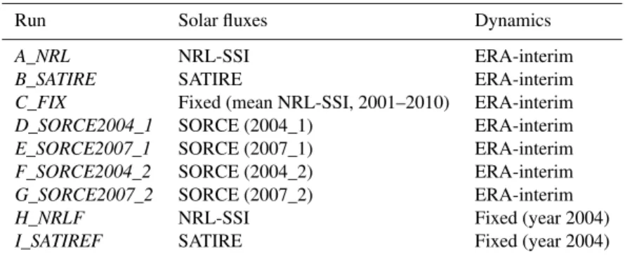
We have performed nine model simulations with dif-ferent solar flux data sets and dynamical conditions, and these are summarised in Table 1. Run A_NRL used NRL-SSI fluxes (similar to run B_Int in Dhomse et al., 2011) while run B_SATIRE used SATIRE-S fluxes for 2001– 2010. Run C_FIX was similar to run A_NRLbut used the mean NRL-SSI fluxes for 2001–2010. This means that run C_FIXonly includes meteorological variability (i.e. no so-lar flux variations). Due to limited time span of the SORCE data time series, a multi-annual simulation could not be performed with these fluxes. Run D_SORCE2004_1 and E_SORCE2007_1 are therefore two separate 10 yr simula-tions with constant SORCE_1 solar fluxes for December 2004 and December 2007, respectively. These are the same fluxes as used in the 2-D model study by Haigh et al. (2010). Two additional simulations with recently updated SORCE_2 solar fluxes are included as run F_SORCE2004_2 and G_SORCE2007_2. RunsH_NRLFandI_SATIREFare simi-lar toA_NRLandB_SATIRE, respectively, but with fixed dy-namics (from year 2004); these runs therefore contain solar variability but no meteorological variability.
4 Results and discussion
The differences in irradiance from the different solar flux data sets used in our model simulations are shown in Fig. 1. The threshold wavelength (242 nm) controlling O3
Table 1.Solar and dynamical conditions for the model simulations. All the runs are performed for the 2001–2010 time period.
Run Solar fluxes Dynamics
A_NRL NRL-SSI ERA-interim
B_SATIRE SATIRE ERA-interim
C_FIX Fixed (mean NRL-SSI, 2001–2010) ERA-interim
D_SORCE2004_1 SORCE (2004_1) ERA-interim
E_SORCE2007_1 SORCE (2007_1) ERA-interim
F_SORCE2004_2 SORCE (2004_2) ERA-interim
G_SORCE2007_2 SORCE (2007_2) ERA-interim
H_NRLF NRL-SSI Fixed (year 2004)
I_SATIREF SATIRE Fixed (year 2004)
dIrradiance (%, (2004-2007)/2004)
100 200 300 400 500
Wavelength (nm) -2
0 2 4 6 8 10 12
DIrradiance (%)
SORCE_1
SORCE_2
NRL
SATIRE
Not Used
*
*
*
Fig. 1. Relative percentage differences in solar irradiance be-tween 2004 and 2007 ((2004–2007)/2004) for the SORCE_1 and SORCE_2 (red and orange diamonds), NRL-SSI (green triangles) and SATIRE (blue circles) solar flux data sets. The threshold wave-length (242 nm) controlling O3production and destruction is indi-cated with a vertical dashed line. Solar flux changes in the Lyman-α line are indicated with stars (∗) on a vertical dashed line at 121.6 nm. Note that runs with SORCE fluxes do not include Lyman-αchanges. Black symbols indicate variations in Schumann–Runge continuum in NRL-SSI and SATIRE data sets but are not included in any of the model simulations.
Woods (2012) and Ermolli et al. (2013) re-evaluated the SORCE data and suggested that the UV variability detected by SORCE might be half of that shown in Fig. 1. DeLand and Cebula (2012) argued that the SORCE_1 flux variations shown in Fig. 1 might be incorrect due to undercorrection of instrument response changes during early on-orbit measure-ments. This indicates ongoing uncertainty in the accuracy of the SORCE data. Therefore, solar flux differences from re-cently updated SORCE_2 data are also shown in Fig. 1. We use both versions of the SORCE data (the one used in Haigh et al. (2010) and the updated one) to test the impact on mod-elled ozone.
There are significant differences between stratospheric and mesospheric O3 chemistry. O3is dynamically controlled in
the lower stratosphere where it is long-lived. In the upper stratosphere, O3 and the odd-oxygen (Ox) family have a
shorter photochemical lifetime, but O3 is still much more
abundant than atomic oxygen, and there is only a weak di-urnal cycle. In contrast, there is a strong didi-urnal cycle in mesospheric O3via HOxchemistry (e.g. Marsh et al., 2003)
with O3 more abundant at night. Figure 2 shows monthly
mean tropical (25◦S–25◦N) daytime and night-time O3
pro-files from SABER, MLS and run A_NRL. Overall, there is good agreement between modelled and observed O3during
both December 2004 and December 2007. However, the peak in modelled O3 seems to be at a lower altitude, and upper
stratospheric O3values are slightly smaller than those from
SABER and MLS. Daytime O3values are in good agreement
in the lower mesosphere, but above 55 km modelled night-time O3mixing ratios are less than observed by SABER or
MLS. The estimated amplitude of the O3diurnal cycle
(day-time mean minus night-(day-time mean) is also shown in Fig. 2. As expected, there are small differences in the stratosphere (up to 0.5 ppm, or 5 %), with the daytime (13:30 UTC) val-ues slightly larger. This is due to differences in the produc-tion and destrucproduc-tion of Oxduring the day with the
produc-tion more strongly peaked in the middle of the day. In the mesosphere the diurnal cycle is larger with nighttime values greater than daytime. This reflects conversion of O to O3at
night. However, the amplitude of the diurnal cycle in mod-elled O3in the mesosphere above 55 km seems to be slightly
Tropical O3 [Dec 2004]
-5 0 5 10
O3 (ppm) 100.0 10.0 1.0 0.1 Pressure [hPa] Day(dashed) Night(solid)
Tropical O3 [Dec 2007]
-5 0 5 10
O3 (ppm) SLIMCAT SABER MLS dSABER (x10) dMLS (x10) dSLIM (x10) @1.30 20 30 40 50 60 ~height [km]
Fig. 2.Monthly mean tropical (25◦S–25◦N) O3profiles for De-cember 2004 and DeDe-cember 2007 from SABER data (black), MLS data (grey) and SLIMCAT runA_NRL(orange). Solid and dashed lines represent night-time and daytime profiles, respectively. Also shown is the O3diurnal variation (night–day) for SABER (green), MLS (violet) and SLIMCAT (light blue). The SLIMCAT differ-ences are shown for 01:30 UTC and 13:30 UTC. For clarity, the di-urnal variations have been multiplied by 10.
Figure 3 shows tropical (25◦S–25◦N) O3 anomalies at
0.3, 3 and 30 hPa from model runsA_NRL,B_SATIRE, and C_FIX (2001–2010) along with SABER (2002–2010) and MLS (2004–2010) observations. Excellent agreement among satellite and modelled O3anomalies is observed at the 3
lev-els with typical differences between them less than 1 %. This is not surprising as middle-lower stratospheric O3is
dynam-ically controlled, and our simulations use realistic dynamics (including the Quasi-Biennial Oscillation or QBO). Overall, the modelled O3anomalies are better correlated with MLS
than SABER. For example, at 30 hPa and 3 hPa, the MLS– model correlation is 0.9 while for MLS–SABER it is 0.8, highlighting the differences in the observational data sets. The MLS–SABER differences are largest in 2005 and 2008. In general, prior to 2005, SABER O3anomalies are slightly
smaller (<0.5 %) than MLS and SLIMCAT at all levels, and they become slightly larger afterwards.
The good correlation between modelled and satellite O3
anomalies provides confidence in the middle and upper stratospheric O3 changes during this period. However, the
weaker correlations in the observational data sets in the lower mesosphere (0.3 hPa) (e.g. Mieruch et al., 2012) suggest that O3changes in this region must be carefully interpreted. Some
model–SABER differences during the first few months of the SABER period might be due to reported ice build-up in the SABER detector during this time (Rong et al., 2009).
Zonal mean O3 mixing ratios for December 2004 from
SLIMCAT (runs A_NRL, C_FIX, D_SORCE2004_1, and F_SORCE2004_2), SABER and MLS are shown in Fig. 4. Results from runB_SATIREare not shown as they are similar to runA_NRL. Although there is generally excellent
agree--10 -5 0 5 10 30hPa (%) A-MLS(0.96) A-SABER(0.76) MLS-SABER(0.86) B-MLS(0.96)
B-SABER(0.77) C-MLS(0.96)C-SABER(0.79)
2002 2004 2006 2008 2010
years -10 -5 0 5 10 3hPa (%) A-MLS(0.90) A-SABER(0.91) MLS-SABER(0.87)B-MLS(0.89) B-SABER(0.91) C-MLS(0.90) C-SABER(0.80) -10 -5 0 5 10 0.3hPa (%)
tropical O3 ano.
A-MLS(0.62) A-SABER(0.39)
MLS-SABER(0.75)
B-MLS(0.61)
B-SABER(0.45) C-MLS(0.60)C-SABER(0.56)
MLS
SABER
A_NRL B_SATIRE C_FIX
Fig. 3.Tropical (25◦S–25◦N) O3anomalies (%) from 3 model sim-ulations (runA_NRL– violet, runB_SATIRE– orange, runC_FIX– green) and satellite data (MLS (2004–2010) – filled circles, SABER (2002–2010) – triangles) at 30 hPa (bottom), 3 hPa (middle) and 0.3 hPa (top). Monthly mean anomalies are calculated by subtract-ing climatological monthly mean values from each monthly mean. The climatological monthly means are over different time periods for individual satellite and model time series. The rank correlation between different O3anomalies is also given.
ment in the O3 distribution, some differences in modelled
and satellite O3in the tropical stratosphere are visible. In the
middle stratosphere (near 10 hPa) MLS values are slightly smaller than SABER and SLIMCAT. In the lower strato-sphere (below 50 hPa) and the lower mesostrato-sphere (above 1 hPa), SABER mixing ratios are larger than SLIMCAT and MLS.
Figure 4 also shows the relative O3 differences between
December 2004 and December 2007. Haigh et al. (2010) showed differences for daytime O3only (their Fig. 2), whilst
our differences shown in Fig. 4 include both daytime and night-time O3. Also, Haigh et al. (2010) used a coupled
dynamical–chemical 2-D model, so a direct comparison with their results cannot be performed. However, some differences in O3between the 2-D model and SLIMCAT (runsA_NRLas
well asD_SORCE2004_1minusE_SORCE2007_1) are no-ticeable. As in Haigh et al. (2010) (with SORCE_1 fluxes), a 2–4 % O3 increase in the tropical middle stratosphere
Fig. 4.Zonal mean monthly mean O3mixing ratio (ppmv) from SLIMCAT runsA_NRL,D_SORCE2004_1,F_SORCE2004_1,C_FIX(a, c,eandg) and SABER and MLS (iandk) for December 2004. The ozone differences (%) between December 2004 and December 2007 for the corresponding data sets are also shown (b,d,f,h,j,l).
significant O3 reductions in the tropical upper stratosphere
(above 1 hPa) produced in the 2-D model with SORCE so-lar fluxes are not visible in MLS, SABER or any SLIM-CAT simulation. Note that both the runs with SORCE fluxes (runsD_SORCE2004_1andF_SORCE2004_2) have larger O3mixing ratios than run A_NRLin December 2004. This
is due to absolute differences between NRL-SSI and SORCE fluxes; the exact cause of this difference in solar fluxes is be-yond the scope of this study.
Another interesting feature in Fig. 4 is the 10 % increase in O3in the range of 0–30◦N and 15–5 hPa, which is distinctly
noticeable in the observations and is well captured by the model. The model also captures the∼10 % less O3between
5◦S–5◦N near 30 hPa, 20–40◦S near 70 hPa, and 70–90◦S near 20 hPa. However, there are differences in the SABER and MLS observations. Enhanced O3 in the tropical lower
stratosphere near 50 hPa is seen by MLS and the model, but does not appear in the SABER data. SABER also observed nearly 2 % less O3 in the Southern Hemisphere (SH)
mid-latitude upper stratosphere (above 0.3 hPa), which is not seen by MLS or reproduced by the model.
To analyse the effect of the diurnal cycle and for bet-ter comparison with Haigh et al. (2010), annual mean daytime and night-time O3 differences between 2004 and
2007 with SORCE fluxes (runs D_SORCE2004_1 mi-nus E_SORCE2007_1) are shown in Fig. 5. Although the most recent SORCE solar fluxes are different to those used by Haigh et al. (2010), this did not lead to any major change to the mean O3 distributions (runs F_SORCE2004_2 and G_SORCE2007_2), so they are not shown here. A middle stratospheric O3 enhancement of
Fig. 5. (a)Differences in annual mean zonal mean O3between 2004 and 2007 forD_SORCE2004_1andE_SORCE2007_1in daytime (i.e. O3change due to both solar flux and dynamical variability). (b)Similar to(a)but for fixed meteorological forcing (year 2004, i.e. O3changes only due to solar flux variability).(c)and(d)are similar to(a)and(b), respectively but for night-time O3.
both daytime and night-time O3 (see also Fig. 4h). Hence
most of these O3changes must be due to dynamical changes.
Interestingly these positive O3differences in the tropics are
much larger than the 2-D model. However, at mid-high lati-tudes SLIMCAT shows negative differences (i.e. more O3in
2007) while the 2-D model showed nearly uniform positive differences throughout the stratosphere. These negative O3
differences are distinctly visible between 40 and 60◦N.
In the upper stratosphere and lower mesosphere, SLIM-CAT does not show any significant O3differences. However,
in a fixed (or identical) dynamics simulation (with different SORCE fluxes), they are slightly negative during the day but become positive at night. For the mean solar signal in O3
in the lower mesosphere, these effects seem to cancel out. This is in disagreement with Merkel et al. (2011), who ar-gued for an insignificant solar signal in night-time O3, and
thus an average O3solar signal remains negative.
Addition-ally, with updated SORCE solar fluxes, SLIMCAT simulates almost 3 % more O3in the middle stratosphere between
De-cember 2004 and DeDe-cember 2007 compared to 1.5 % using older SORCE fluxes (not shown).
Figure 6 shows daytime and night-time O3differences
be-tween 2003–2004 and 2008–2009 from model runsA_NRL, B_SATIRE,C_FIXand SABER. We have selected the pairs of years as active and quiet solar periods in order to make a direct comparison with the results from Merkel et al. (2011). Again, the O3 difference patterns between
obser-vational and modelled data are nearly similar. The SABER data and all three model simulations show 3–6 % more O3
in the tropical middle stratosphere during 2003–2004 com-pared to 2008–2009. Negative differences in the lower
strato-Fig. 6.Daytime(a–d)and night-time(e–h)biannual mean zonal mean O3differences (%) between 2003/2004 and 2008/2009 for (a ande) SLIMCAT runA_NRL, (bandf) SLIMCAT runB_SATIRE, (candg) SLIMCAT runC_FIXand (dandh) SABER data.
sphere (near 50 hPa) are also in agreement between the data and model runs. The simulations show negligible (<1 %) O3 differences in the upper stratosphere and lower mesosphere. SABER also shows nearly 0.5 % negative O3 anomalies in
a narrow region near 0.3 hPa in both daytime and night-time data. SH mid-latitude SABER-observed O3changes are
better captured in runB_SATIREthan runA_NRL, whereas NH mid-latitude changes are in better agreement with run A_NRL. However, due to the limited spatial coverage of SABER measurements, mid-latitude O3 differences are not
discussed here.
As expected, our analysis of SABER data shown in Fig. 6 is consistent with the active (2003/2004) and quiet (2008/2009) period O3 differences shown in Figure 2 of
Merkel et al. (2011). However, the SLIMCAT O3
a) SMAX-SMIN O3 (%)
-5 0 5
dO3 per solar cycle (%) 100.0
10.0 1.0 0.1
Pressure [hPa]
HALOE (Remsberg,2008) 2D (Brasseur,1993)
C-SLIMCAT (Dhomse et al., 2011)
A-SLIMCAT (Dhomse et al., 2011)
SAGE-based(RW2007) SBUV/SAGE(Mc2009)
b)Solar response (regres)
-5 0 5
dO3 per solar cycle (%) SABER
MLS SLIM_A
SLIM_B SLIM_C
c)Solar response (regres)
-5 0 5
dO3 per solar cycle (%)
SLIM_H (FixD)
SLIM_I (FixD)
SLIM_A (8yrs)
SLIM_B (8yrs) SLIM_C (8yrs)
20 30 40 50 60
~height [km]
Fig. 7. (a)Tropical solar signal (25◦S–25◦N) per solar cycle from SLIMCAT simulations for 1979–2010 with ERA-40 and fixed dynamics (Dhomse et al., 2011, green and red lines), HALOE (1992–2005, Remsberg, 2008, black line) and a 2-D model (Brasseur, 1993, blue line). The estimated solar signals using SBUV/SAGE data (McLinden et al., 2009, triangles), SAGE-based data (Randel and Wu, 2007, stars) and a 3-D model (light-green line) by Dhomse et al. (2011) for 1979–2005 are also shown.(b)Estimated solar signal using multivariate regression model for modelled (2001–2010, 120 months), SABER (2002–2010, 108 months) and MLS (2004–2010, 77 months) O3data sets. Estimated errors (1σ) for solar coefficients are shown with coloured horizontal lines. The large error bars (±10 %) at all levels for MLS data and in the lower stratosphere for SABER and model data are not shown.(c)The coloured dashed lines with filled circles show the solar signal from runsA_NRLandB_SATIREif only 8 yr (2003–2010) of model data are used. The estimated solar signals from the runs (fixed dynamics) H_NRLFandI_SATIREFare shown with dark and light blue lines, respectively.
with NRL-SSI or SORCE solar fluxes shown by Merkel et al. (2011) are less than 1 %, whereas our simulations and SABER show around 2–4 % O3differences. A good
agree-ment between SLIMCAT and observations is expected as we use analysed winds and temperatures, whereas WACCM is a coupled model and therefore can calculate the coupled so-lar response. So difference reported in Merkel et al. (2011) might be coupled dynamical response. However, this again highlights that robust positive O3 anomalies observed in
SABER data can be reproduced in SLIMCAT with either NRL-SSI or SATIRE solar fluxes. Negligible upper strato-spheric lower mesostrato-spheric O3changes with NRL-SSI are in
good agreement with their simulations (see Figure 2a and e in Merkel et al., 2011).
Figure 7a shows the solar signals from some earlier stud-ies (e.g. HALOE (Remsberg, 2008), a 2-D model (Brasseur, 1993) and a 3-D model (Dhomse et al., 2011)). A mid-stratospheric solar signal in earlier SLIMCAT simulations with NRL-SSI fluxes is consistent with other modelling stud-ies (e.g. Austin et al., 2008, see Figure 4). Figure 7b shows the estimated solar signal in tropical (25◦S–25◦N) O3
us-ing modelled and observed O3 anomalies from this study.
The regression model used here is similar to the one used in
Dhomse et al. (2011) containing linear trend, QBO and solar (F10.7flux) terms (see also Dhomse et al., 2006). Overall the
solar signals from runsA_NRLandB_SATIREare in good agreement with SABER (and HALOE) data. However, due to the short time span of available MLS data (77 months), the estimated errors in the MLS solar signal are much larger. A robust positive solar signal in the middle stratosphere is clearly visible in the model simulations as well as SABER and MLS data sets.
There are some differences in the solar signals estimated from modelled and observed O3in Fig. 7b, but they are
statis-tically insignificant. For example, the secondary solar signal maxima in the tropical lower stratospheric O3 observed in
SBUV, SAGE and SLIMCAT are not visible in SABER and MLS data. In the upper stratosphere and lower mesosphere, modelled O3shows a positive (∼1 %) solar signal, whereas
in the observational data it is negative (∼ −1 %). Some of these differences might be due to ice contamination in the SABER detector as discussed earlier.
signal. Figure 7c also shows the “chemical-only” solar re-sponse for the 2001–2010 period from fixed dynamical sim-ulations (runsH_NRLF and I_SATIREF). Again, the solar signal from these simulations shows quite good agreement with the solar signal from SAGE and SBUV data (Soukharev and Hood, 2006). However, its magnitude is less than that for the fixed dynamical simulations presented in Dhomse et al. (2011). This is in line with our expectations, as the 2001–2010 time period only partially covers the solar cycle.
5 Conclusions
When using either NRL-SSI or SATIRE-S solar fluxes, and ECMWF meteorology, simulated O3 from our 3-D CTM
shows excellent agreement with satellite observations for 2001–2010. The model is also able to reproduce changes over the recent 2004–2007 time period, which has previously been used to support the different solar flux variability mea-sured by SORCE. Therefore, our model runs do not provide any indirect support for the accuracy of the SORCE fluxes; rather they argue that the previously accepted NRL-SSI or SATIRE-S fluxes are able to reproduce recent observed O3
changes.
The good agreement between our model and observations is partly due to variability imposed by the ECMWF analy-ses, which is therefore dynamical in origin. However, since 2001, there have been step-wise changes in stratospheric cir-culation (e.g. Dhomse et al., 2008), and there was a major sudden stratospheric warming in the SH in September 2002 (e.g. Weber et al., 2003). It will require further research using a coupled chemistry–climate model to see if these anomalous changes in stratospheric circulation are indeed solar-induced or due to internal atmospheric variability or anthropogenic origin.
Our modelled O3 solar signal in the middle and upper
stratosphere during the 2001–2010 time period is different to that deduced from SBUV or SAGE data (1979–2003), but only slightly different (similar structure but larger in magni-tude) to HALOE (1992–2005). However, there are some un-certainties in the SBUV (e.g. poor vertical resolution) and SAGE (e.g. limited temporal sampling, Twomey–Chahine inversion near 50 km) data sets (e.g. Terao and Logan, 2007; Wang et al., 2011). A re-evaluation of SBUV and SAGE data is needed to confirm if the solar signal in stratospheric O3
during the recent solar cycle is indeed out of phase with TSI changes. Overall, our simulations suggest that an out-of-phase solar signal in the lower mesospheric O3during recent
solar cycle cannot be used to distinguish between the various solar flux data sets due to large uncertainties and the short time span of the observations.
Acknowledgements. We thank NASA for the MLS and SABER O3 data sets. We also acknowledge use of the ECMWF data, which was obtained via the BADC. This work was supported by the
NERC SOLCLI project, STFC, NCAS and NCEO. The National Center for Atmospheric Research is sponsored by the National Science Foundation.
Edited by: Q. Errer
References
Austin, J., Tourpali, K., Rozanov, E., Akiyoshi, H., Bekki, S., Bodeker, G., Bruehl, C., Butchart, N., Chipperfield, M., Deushi, M., Fomichev, V. I., Giorgetta, M. A., Gray, L., Kodera, K., Lott, F., Manzini, E., Marsh, D., Matthes, K., Nagashima, T., Shibata, K., Stolarski, R. S., Struthers, G. H., and Tian, W.: Coupled chemistry climate model simulations of the solar cy-cle in ozone and temperature, J. Geophys. Res., 113, D11306, doi:10.1029/2007JD009391, 2008.
Ball, W. T., Unruh, Y., Krivova, N. A., Solanki, S., Wenzler, T., Mortlock, D. J., and Jaffe, A. H.: Reconstruction of to-tal solar irradiance 1974–2009, Astron. Astrophys., 541, A37, doi:10.1051/0004-6361/201118702, 2012.
Brasseur, G.: The response of the middle atmosphere to long-term and short-term solar variability: A two-dimensional model, J. Geophys. Res., 98, 23079–23090, 1993.
Brasseur, G. and Solomon, S.: Aeronomy of the middle atmosphere, D. Reidel Publishing Company, 1984.
Briegleb, B. P.: Delta-Eddington approximation for solar radiation in the NCAR Community Climate Model, J. Geophys. Res., 97, 7603–7612, 1992.
Chipperfield, M. P.: New Version of the TOMCAT/SLIMCAT Off-Line Chemical Transport Model: Intercomparison of Strato-spheric Tracer Experiments, Q. J. Roy. Meteor. Soc., 132, 1179– 1203, 2006.
Dee, D. P., Uppala, S. M., Simmons, A. J., Berrisford, P., Poli, P., Kobayashi, S., Andrae, U., Balmaseda, M. A., Balsamo, G., Bauer, P., Bechtold, P., Beljaars, A. C. M., van de Berg, L., Bid-lot, J., Bormann, N., Delsol, C., Dragani, R., Fuentes, M., Geer, A. J., Haimberger, L., Healy, S., Hersbach, H., Holm, E. V., Isak-sen, L., Kayllberg, P., Koehler, M., Matricardi, M., McNally, A. P., Monge-Sanz, B. M., Morcrette, J.-J., Peubey, C., de Ros-nay, P., Tavolato, C., Thépaut, J.-N., and Vitart, F.: The ERA-Interim reanalysis: Configuration and performance of the data assimilation system, Q. J. Roy. Meteor. Soc., 133, 1972–1990, 2011.
DeLand, M. T. and Cebula, R. P.: Solar UV variations during the de-cline of Cycle 23, J. Atmos. Sol.-Terr. Phys., 77, 225–234, 2012. Dhomse, S., Weber, M., Wohltmann, I., Rex, M., and Burrows, J. P.: On the possible causes of recent increases in northern hemispheric total ozone from a statistical analysis of satellite data from 1979 to 2003, Atmos. Chem. Phys., 6, 1165–1180, doi:10.5194/acp-6-1165-2006, 2006.
Dhomse, S., Weber, M., and Burrows, J.: The relationship between tropospheric wave forcing and tropical lower stratospheric water vapor, Atmos. Chem. Phys., 8, 471–480, doi:10.5194/acp-8-471-2008, 2008.
Ermolli, I., Matthes, K., Dudok de Wit, T., Krivova, N. A., Tourpali, K., Weber, M., Unruh, Y. C., Gray, L., Langematz, U., Pilewskie, P., Rozanov, E., Schmutz, W., Shapiro, A., Solanki, S. K., and Woods, T. N.: Recent variability of the solar spectral irradiance and its impact on climate modelling, Atmos. Chem. Phys., 13, 3945–3977, doi:10.5194/acp-13-3945-2013, 2013.
Froidevaux, L., Jiang, Y. B., Lambert, A., Livesey, N. J., Read, W. G., Waters, J. W., Browell, E. V., Hair, J. W., Avery, M. A., Mcgee, T. J., Twigg, L. W., Sumnicht, G. K., Jucks, K. W., Margitan, J. J., Sen, B., Stachnik, R. A., Toon, G. C., Bernath, P. F., Boone, C. D., Walker, K. A., Filipiak, M. J., Harwood, R. S., Fuller, R. A., Manney, G. L., Schwartz, M. J., Daffer, W. H., Drouin, B. J., Cofield, R. E., Cuddy, D. T., Jarnot, R. F., Knosp, B. W., Perun, V. S., Snyder, W. V., Stek, P. C., Thurstans, R. P., and Wagner, P. A.: Validation of Aura Microwave Limb Sounder stratospheric ozone measurements, J. Geophys. Res., 113, D15S20, doi:10.1029/2007JD008771, 2008.
Gray, L., Beer, J., M., G., Haigh, J., Lockwood, M., Matthes, K., Cubasch, U., Fleitmann, D., Harrison, G., Hood, L., Luter-bacher, J., Meehl, G., Shindell, D., van Geel, B., and White, W.: Solar Influences on Climate, Rev. Geophys., 48, RG4001, doi:10.1029/2009RG000282, 2010.
Haigh, J. D., Winning, A. R., Toumi, R., and Harder, J. W.: An influ-ence of solar spectral variations on radiative forcing of climate, Nature, 467, 696–699, 2010.
Harder, J., Thuillier, G., Richard, E., Brown, S., Lykke, K., Snow, M., McClintock, W., Fontenla, J., Woods, T., and Pilewskie, P.: The SORCE SIM solar spectrum: Comparison with recent obser-vations, Sol. Phys., 263, 3–24, 2010.
Harder, J. W., Fontenla, J. M., Pilewskie, P., Richard, E. C., and Woods, T. N.: Trends in solar spectral irradiance variability in the visible and infrared, Geophys. Res. Lett., 36, L07801, doi:10.1029/2008GL036797, 2009.
Krivova, N., Solanki, S., Fligge, M., and Unruh, Y. C.: Reconstruc-tion of solar irradiance variaReconstruc-tions in cycle 23: Is solar surface magnetism the cause?, Astron. Astrophys., 399, 1–4, 2003. Krivova, N., Solanki, S., and Floyd, L.: Reconstruction of solar
UV irradiance in cycle 23, Astron. Astrophys., 452, 631–639, doi:10.1051/0004-6361:20064809, 2006.
Lary, D. and Pyle, J.: Diffuse radiation, twilight, and photochemistry-I, J. Atmos. Chem., 13, 373–392, 1991. Lean, J. L., Rottman, G. J., Kyle, H. L., Woods, T. N., Hickey, J. R.,
and Puga, L. C.: Detection and parameterization of variations in solar mid- and near-ultraviolet radiation (200–400 nm), J. Geo-phys. Res, 102, 29939–29956, 1997.
Marsh, D., Smith, A., and Noble, E.: Mesospheric ozone re-sponse to changes in water vapor, J. Geophys. Res., 108, 4109, doi:10.1029/2002JD002705, 2003.
McClintock, W. E., Rottman, G. J., and Woods, T. N.: Solar-stellar irradiance comparison experiment II (SOLSTICE II): instrument concept and design, in: The Solar Radiation and Climate Exper-iment (SORCE), 225–258, Springer, 2005.
McLinden, C. A., Tegtmeier, S., and Fioletov, V.: Technical Note: A SAGE-corrected SBUV zonal-mean ozone data set, At-mos. Chem. Phys., 9, 7963–7972, doi:10.5194/acp-9-7963-2009, 2009.
Merkel, A. W., Harder, J. W., Marsh, D. R., Smith, A. K., Fontenla, J. M., and Woods, T.: The impact of solar spectral irradiance
vari-ability on middle atmospheric ozone, Geophys. Res. Lett., 38, L13802, doi:10.1029/2011GL047561, 2011.
Mieruch, S., Weber, M., von Savigny, C., Rozanov, A., Bovens-mann, H., Burrows, J. P., Bernath, P. F., Boone, C. D., Froide-vaux, L., Gordley, L. L., Mlynczak, M. G., Russell III, J. M., Thomason, L. W., Walker, K. A., and Zawodny, J. M.: Global and long-term comparison of SCIAMACHY limb ozone profiles with correlative satellite data (2002–2008), Atmos. Meas. Tech., 5, 771–788, doi:10.5194/amt-5-771-2012, 2012.
Minschwaner, K., Salawitch, R., and McElroy, M.: Absorption of solar radiation by O2: Implications for O3and lifetimes of N2O, CFCl3, and CF2Cl2, J. Geophys. Res., 98, 10543–10561, 1993. Oberländer, S., Langematz, U., Matthes, K., Kunze, M., Kubin, A.,
Harder, J., Krivova, N. A., Solanki, S. K., Pagaran, J., and We-ber, M.: The influence of spectral solar irradiance data on strato-spheric heating rates during the 11 year solar cycle, Geophys. Res. Lett., 39, L01801, doi:10.1029/2011GL049539, 2012. Randel, W. J. and Wu, F.: A stratospheric ozone profile
data set for 1979-2005: Variability, trends, and comparisons with column ozone data, J. Geophys. Res., 112, D06313, doi:10.1029/2006JD007339, 2007.
Remsberg, E. E.: On the response of Halogen Occultation Ex-periment (HALOE) stratospheric ozone and temperature to the 11-year solar cycle forcing, J. Geophys. Res., 113, D22304, doi:10.1029/2008JD010189, 2008.
Rong, P. P., Russell III, J. M., Mlynczak, M. G., Remsberg, E. E., Marshall, B. T., Gordley, L. L., and López-Puertas, M.: Validation of Thermosphere Ionosphere Mesosphere Energetics and Dynamics/Sounding of the Atmosphere using Broadband Emission Radiometry (TIMED/SABER) v1.07 ozone at 9.6 µm in altitude range 15–70 km, J. Geophys. Res., 114, D04306, doi:10.1029/2008JD010073, 2009.
Rottman, G.: The SORCE mission, in: The Solar Radiation and Cli-mate Experiment (SORCE), 7–25, Springer, 2005.
Russell III, J. M., Mlynczak, M. G., Gordley, L. L., Tansock Jr, J. J., and Esplin, R. W.: Overview of the SABER experiment and pre-liminary calibration results, in: SPIE’s International Symposium on Optical Science, Engineering, and Instrumentation, 277–288, International Society for Optics and Photonics, 1999.
Soukharev, B. E. and Hood, L. L.: Solar cycle variation of strato-spheric ozone: Multiple regression analysis of long-term satellite data sets and comparisons with models, J. Geophys. Res., 111, D20314, doi:10.1029/2006JD007107, 2006.
Terao, Y. and Logan, J. A.: Consistency of time series and trends of stratospheric ozone as seen by ozonesondes, SAGE II, HALOE, and SBUV(/2), J. Geophys. Res., 112, D06310, doi:10.1029/2006JD007667, 2007.
Unruh, Y., Solanki, S., and Fligge, M.: The spectral dependence of facular contrast and solar irradiance variations, Astron. Astro-phys., 345, 635–642, 1999.
Weber, M., Dhomse, S., Wittrock, F., Richter, A., Sinnhuber, B., and Burrows, J.: Dynamical control of NH and SH winter/spring total ozone from GOME observations in 1995–2002, Geophys. Res. Lett., 30, 1583, doi:10.1029/2002GL016799, 2003. WMO: Scientific Assessment of Ozone Depletion: 1985, Global
Ozone Research and Monitoring Project Report 16, World Mete-orological Organization, Geneva, 1985.