Exploiting the Adaptation Dynamics to Predict the Distribution of Beneficial Fitness Effects.

Exploiting the Adaptation Dynamics to

Predict the Distribution of Beneficial Fitness

Effects

Sona John*☯, Sarada Seetharaman☯

Theoretical Sciences Unit, Jawaharlal Nehru Centre for Advanced Scientific Research, Jakkur P.O., Bangalore 560064, India

☯These authors contributed equally to this work. *sonajohn@jncasr.ac.in

Abstract

Adaptation of asexual populations is driven by beneficial mutations and therefore the dynamics of this process, besides other factors, depends on the distribution of beneficial fitness effects. It is known that on uncorrelated fitness landscapes, this distribution can only be of three types: truncated, exponential and power law. We performed extensive sto-chastic simulations to study the adaptation dynamics on rugged fitness landscapes, and identified two quantities that can be used to distinguish the underlying distribution of benefi-cial fitness effects. The first quantity studied here is the fitness difference between succes-sive mutations that spread in the population, which is found to decrease in the case of truncated distributions, remains nearly a constant for exponentially decaying distributions and increases when the fitness distribution decays as a power law. The second quantity of interest, namely, the rate of change of fitness with time also shows quantitatively different behaviour for different beneficial fitness distributions. The patterns displayed by the two aforementioned quantities are found to hold good for both low and high mutation rates. We discuss how these patterns can be exploited to determine the distribution of beneficial fit-ness effects in microbial experiments.

Introduction

Microbial populations have to constantly adapt in order to survive in a changing environment. For example, a bacterial population exposed to a new antibiotic must evolve in order to exist [1]. In asexual populations, this process of adaptation is driven only by rare beneficial muta-tions [2] which provide fitness advantage. Therefore, in order to survive in a new environment, enough beneficial mutations should be available and the beneficial mutations should confer sufficient fitness advantage. While the first factor depends on the mutation rate and population size, the second factor is determined by the underlying fitness distributions. Even though we have some understanding about the mutation rate of different microbial populations, the full fitness distribution is more complex and relatively little is known about it. However, for

OPEN ACCESS

Citation:John S, Seetharaman S (2016) Exploiting the Adaptation Dynamics to Predict the Distribution of Beneficial Fitness Effects. PLoS ONE 11(3): e0151795. doi:10.1371/journal.pone.0151795

Editor:Frederick M. Cohan, Wesleyan University, UNITED STATES

Received:February 15, 2015

Accepted:March 4, 2016

Published:March 18, 2016

Copyright:© 2016 John, Seetharaman. This is an open access article distributed under the terms of the

Creative Commons Attribution License, which permits unrestricted use, distribution, and reproduction in any medium, provided the original author and source are credited.

Data Availability Statement:All relevant data are within the paper and its Supporting Information files.

Funding:The authors have no support or funding to report.

moderately adapted populations (i.e., fitness of the wild type is high enough), rare beneficial mutations which occur in the tail of the fitness distribution can be described by the extreme value theory (EVT) as proposed first by Gillespie [3]. The EVT states that the extreme tail of all distributions of uncorrelated random variables (fitness, in this case) can be of only three types. Depending on whether the tail of underlying fitness distribution is truncated or decaying faster than a power law or as a power law, the EVT distribution would belong to the Weibull or Gum-bel or Fréchet domain, respectively [4]. All three EVT domains can be obtained from the gener-alized Pareto distribution given as

pðfÞ ¼ ð1_þkfÞ 1þkk_; ð1Þ

whereκis the tuning parameter. One example from each of the three EVT domains is shown

inFig 1, which shows the distribution of beneficial effectsp(f) withfitnessf. The three types of EVT domains are classified according to the value ofκ. Here negativeκbelongs to the Weibull

domain, whileκ= 0 corresponds to the Gumbel domain and positiveκto the Fréchet domain.

Interestingly, all three distribution of beneficialfitness effects(DBFEs) have been observed in experiments on microbial populations [5–14]. While the exponential distribution belonging to the Gumbel domain has been most commonly seen [5–8], in recent times, the distribution of beneficial mutations belonging to the Weibull [10,14] and Fréchet [11] domains have also been observed.

Recent theoretical studies have shown analytically and numerically that qualitatively differ-ent patterns occur in the adaptation dynamics of populations in differdiffer-ent EVT domains of DBFEs in a low mutation regime [15–18]. Specifically, it has been shown that fitness gain in a fixation event follows the pattern of diminishing returns in the Weibull domain, constant returns in the Gumbel domain and accelerating returns in the Fréchet domain, and thus indi-cates that this quantity can be used to predict the DBFE. These observations are restricted to strong selection-weak mutation (SSWM) regime in which the genetic variation in the popula-tion is minimal, that is, only one beneficial mutapopula-tion is present in the populapopula-tion in the time interval between its appearance and fixation [7]. It is then natural to ask whether the relation-ship between adaptation dynamics and the DBFE mentioned above are robust for large popula-tions, where there might be more than one beneficial mutation competing for dominance in the population. The main aim of our study is to address this question and to see if the fitness gain in a fixation event can be used for predicting the DBFE in a more general scenario.

Here, we are mainly concerned with the populations in which a large number of mutants are produced at every generation. Hence, more than one beneficial mutation is expected to be present at the same time [19–23]. In this case, the beneficial mutations will compete with each other as has been observed in different experimental populations [24–27]. In this high muta-tion regime, as a result of the competimuta-tion among the beneficial mutamuta-tions, the rate of adapta-tion slows down. Fitness advantage due to the mutaadapta-tions that get fixed is much higher, since the availability of more mutations results in allowing only the best (fittest) mutation to get fixed [28]. A clear comparison of the population fraction of new mutants appearing in a popu-lation for two mutation regimes is given inFig 2. InFig 2(a)we see that the population in the SSWM regime is more or less monomorphic with only one mutant present at a time in all the three EVT domains. However, in a high mutation regime, the population is polymorphic with more than one mutant produced in it at every generation as shown inFig 2(b). In fact, a large amount of genetic variation is observed in the case of bounded distributions corresponding to

κ<0 inEq (1)resulting in a strong competition between the beneficial mutants.

main motivation of this study is to look for quantities which can be used to distinguish between DBFEs using the properties of adaptation dynamics as opposed to the direct measurements of DBFEs. Our most important and interesting result is concerned with the fitness difference between mutations that spread in a population. This quantity shows qualitatively different trends in three EVT domains and thus helps in distinguishing the DBFEs.

We have also studied another quantity which is the rate of change of fitness with time, and observed that this shows quantitatively different behaviour for different EVT domains of the DBFEs. Though some results for the rate of change of fitness are already known in the litera-ture [29], we measured it for all the three cases (Weibull, Gumbel and Fréchet) and identified that this can be used to distinguish the DBFEs in both SSWM and high mutation regimes. In order to obtain a complete picture, a comparison of our study with the existing literature is given inTable 1below.

We also measured quantities like the genetic variation and the number of mutations in the most populated sequence. All of these quantities are discussed in the Results section. We sug-gest that the distinct trends shown by the above mentioned quantities can be used to predict

Fig 1. The figure shows the distribution of beneficial fitness effectsp(f) with fitnessffor the three EVT domains, given byEq (1)for variousκ.Here,

DBFEs from experimental studies on adaptation. The relevance of our work to experiments is also explored in the Discussion section.

Materials and Methods

We track the dynamics of a population of self-replicating (asexual), infinitely long binary sequences of fixed size using the standard Wright-Fisher process [21,28]. In our work, the pop-ulation size is held constant atN= 104, unless specified otherwise and the total mutation prob-ability (beneficial and deleterious) per sequence is given byμ. Every occupied sequence is

counted as aclassand is labeled when it arises in the population. Initially, the whole population is in class 1 whose fitness is fixed and specified in every simulation run. We have used the term leader to refer to the class whose normalised probability of reproduction (product of popula-tion fracpopula-tion and fitness) is greater than half. In that case, clearly class 1 is the initial leader since the whole population is localized there. At every time step, out ofNsequences,mtare

chosen from a binomial distribution with meanNμas mutants. Every mutant produced

increases the number of classes in the population by one, and with time, the mutants may pro-duce their own set of further mutants. The population fraction of each class may grow or go extinct, as can be observed inFig 2. At any timet, the number of classes present in the popula-tion is given byN

cðtÞ, and the population size andfitness of each class,i, where1iNc, is

Fig 2. Population fraction of different mutant classes are shown as different coloured lines, where (a) shows the SSWM (Nμ= 0.1, low mutation

rate) regime and (b) shows the high mutation (Nμ= 10) regime for all three EVT domains of DBFE.

doi:10.1371/journal.pone.0151795.g002

Table 1. Comparison with existing literature.Here,Dfstepis the averagefitness difference between the present leader and the new beneficial mutation that

gets established and_{FðtÞis the rate of change offitness.}

Quantities DBFE domains: Low mutation regime DBFE domains: High mutation regime

Weibull Gumbel Fréchet Weibull Gumbel Fréchet

Df_step [16] [16] [16] this study this study this study

FðtÞ this study [29] [29] this study [29] this study

denoted byn(i,t) andf(i), respectively. The normalized probability of each class at every time step,~_{pði;tÞcontributing offspring to the population at the next time step, depends on the} pop-ulation size of the class at the present time step and thefitness of the class as

~

pði;tÞ ¼ nði;tÞfðiÞ SNcðtÞ

j¼1 nðj;tÞfðjÞ

: ð2Þ

Note that though thefitness of the class is the same as long as it persists in the population, its size may vary at every time step, thus changing its probability of reproduction as given byEq (2). Different classes are populated in the next time step based on the multinomial distribution

Pðnð1;t0_Þ;nð2;t0_Þ::nðN

c;t

0_{ÞÞ ¼N!}Y

N_cðtÞ

j¼1

½~_pðj;tފnðj;tÞ

nðj;tÞ! ; ð3Þ

wheret0=t+ 1. The above equation is subject to the constraintSNcðtÞ

j¼1 nðj;t0Þ ¼N. In our

simu-lations, we implementEq (3)along with the above constraint by convertingEq (3)to a bino-mial distribution for every class,1_i<N

cðtÞas

nði;t0Þ ¼ ~

NðiÞ

nði;tÞ

!

qði;tÞnði;tÞ

ð1 _qði;tÞÞN~ðiÞ nði;tÞ

: ð4Þ

We set the population size of the last class asnðN

cðtÞ;t0Þ ¼N

PNcðtÞ 1

i¼1 nði;t0Þ. InEq (4),

qði;tÞ ¼ ~

pði;tÞ SNcðtÞ

j¼i p~ðj;tÞ

; ð5Þ

andN~ðiÞ ¼N Sij¼11nðj;tÞ.

At every time step, once the classes are populated based on the algorithm described above,

mtsequences are chosen as mutants based on the binomial distribution with meanNμ. Every

new mutant class that appears in the population reduces the population size of the class in which it arose by one. In our work, we have variedμto access both the SSWM (low mutation)

and the high mutation regime. In our simulations unless specified otherwise,Nμ= 0.01 in low

(SSWM) andNμ= 50 in high mutation regimes.

A new class is assigned to each mutant and its fitness is chosen from a generalized Pareto distribution [4] given inEq (1). The advantage of usingEq (1)is that we can access all three EVT domains of DBFE by changingκ. The distributions whoseκ<0 belong to the Weibull domain, whileκ= 0 belong to the Gumbel domain, andκ_>0 belong to the Fréchet domain,

respectively. The frequency distribution of beneficial effectsp(f) for various values ofκis

shown inFig 1. The upper boundufor the distributions chosen fromEq (1)is infinity when

κ0 and equals₋1/κforκ<0. In this work, the fitness of the mutants is independently cho-sen fromEq (1)thus making the fitness of the mutant,Fman uncorrelated variable, which may

be greater or smaller than the parent fitness,Fp. We have analyzed the results to see how they

vary between the three EVT domains and different mutation rates.

In the allocation of the fitness to any mutant, our work differs from the other works on clonal interference [21,28] wherein the fitness of the mutant is hiked above the parent fitness by the selection coefficients (s) which may be held constant or chosen from a distribution as

Fm= (1 +s)Fp. Unlike the model we have used in this work (as explained above), in this case,

there is a strong correlation between the mutant fitnessFmand the parent fitnessFp. In those

as the fitness of the parent increases, the number of better mutants available decreases thus producing different patterns for the fitness increment in each EVT domain.

In our model, whenever a mutant class goes extinct, the classes below it are moved up and the number of classes in the population is reduced by one. The normalised probability of repro-duction given inEq (2)of a class exceeding half corresponds to a leader change. The new leader determined now belongs to the class whose normalised probability exceeded half. We have also explored other criteria for defining the leader as the most populated class and find that our main results are robust with respect to the change in criteria (data not shown).

Every change of a leader is counted as astep. In the high mutation regime, the population is spread over many sequences and a sequence can produce two or more mutants, each of which may become leaders at different time steps. However, in the SSWM regime, the whole popula-tion is localised at a single sequence with a fixed fitness and can only move to a different sequence with higher fitness one mutation away. Thus every new leader arises from the previ-ous leader, as can be observed inFig 2(a). When a better sequence appearing in the population does not get lost due to genetic drift, it quickly gets fixed. Further mutations that may lead to future leaders appear in this genetic background. The change in the fitness of the population is the same as the change in the fitness of the leader. In this case, every move of the population (leader) from one sequence to another is termed as a step in the adaptive walk [30–33], whereas in the high mutation regime, the population is polymorphic and as seen fromFig 2(b)the leader change is not obvious.

Various quantities like the difference in fitness between successive leaders and the average number of mutations in the leader are averaged only over the walks that take the step. Other quantities like the number of classes present at any point in time and the rate of change of fit-ness are averaged over all time steps in that simulation run.

In this paper, the total number of iterations is 105in every simulation run and the dynamics are tracked for a finite time limit of 104generations, which we shall refer to astmax. In this time

span, the maximum fitness value,fmaxthat arises in the population can be calculated as

tmaxNm

Z u fmax

pðfÞdf ¼1; ð6Þ

whereuis the upper limit of thefitness distribution equalling (-1/κ) for bounded distributions

and infinity for the unbounded ones [4]. From the above integral, we get

fmax¼

ðtmaxNmÞ

k ₁

k

: ð7Þ

Results

The number of classes in the population

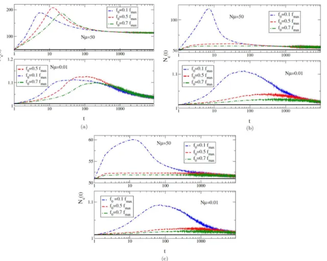
For a population that is fixed in size, the number of classes in the population is expected to increase with the mutation rate. The average genetic variation, which is defined here as the average number of classes (N

c) present in the population is shown inFig 3for all three DBFE

class is quickly replaced by afitter mutant and all further mutants that arise on this new back-ground must compete with thisfitter class.

In the low mutation regime, the population is localized at a single sequence for most of the time and producesNμmutants at every time step. Hence, in this case, the average number of

classes approach a constantNμ+ 1 at large times as can be seen in the bottom panels ofFig 3.

These panels also indicate that the value of this constant increases with decreasingκ. This is

because in the case of bounded distributions withκ_<0, the fitness of a beneficial mutant

pro-duced is expected to be closer to the parent fitness. In other words, mutations are nearly neutral and thus it takes a longer time to take over the population as shown inFig 2(a). This results in a larger number of mutants in the Weibull domain, which can be observed in the bottom panel ofFig 3(a). We can clearly see from the top panels ofFig 3that number of classes increases with decreasingκeven in a high mutation regime. Moreover, the average number of classes

present at a time is much higher in this regime. This makes sense because the fitness of the clas-ses belonging toκ=₋1 cannot be very different from each other (can take on values between 0

and 1), which makes it possible for many of them to exist in the population. The maximum fit-ness of the classes belonging toκ= 1/4 distribution will on an average be much higher than all

others (since the distribution is unbounded with a fat tail), thus out-competing the others in the population.

Fig 3. The plot shows the average number of classes in the population as function of time for various initial fitnesses.The fitnesses are chosen from Eq (1)with (a)κ=−1 (b)κ!0 and (c)κ= 1/4. For eachκvalue, the plot showsNcðtÞin both high mutation (top panels) and low mutation (bottom panels)

regimes. The straight line in all plots showsNμ+ 1.

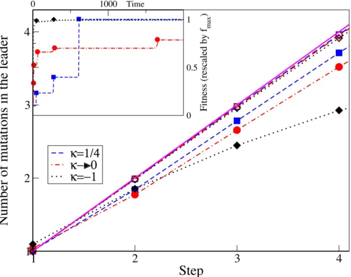
Number of mutations in the leader

In the low mutation regime, the average number of mutations in the leader is expected to be very close to the step number since the genetic variation in the population is low and any muta-tion that escapes drift quickly takes over the populamuta-tion [3]. We verify this point via simula-tions as depicted inFig 4. We find that the mutation number equals the step number in all the three EVT domains of the DBFE in the low mutation regime during the initial steps. However in the high mutation regime, the number of mutations in the leader of any step differs between the three DBFE domains. When the mutation rate is increased, the genetic variation of the pop-ulation and the significance of clonal interference also increases. In the high mutation regime, the number of mutations in the leader is found to be less than the step number in all three DBFE domains. This is because there is a chance that different mutants originating from the same parent class can become the leader of the population at different times. This decrease from the step number is the minimum for the fat-tailed distributions and maximum for the truncated ones, as shown inFig 4. This result is consistent with the number of classes present in the population as discussed in the previous section. In the Fréchet domain, since the clonal interference is minimal, it is most likely that a mutant originating from the present leader will become the next one. In the Weibull domain, due to the large number of classes present in the population, mutants originating from the same class can become leaders at different time points.

Fitness and fitness difference

From our simulations, we find that the average fitness of the first mutant fixed in the popula-tion,f1increases linearly with initialfitness,f0for allκin the low mutation regime and for κ6¼0 in the high mutation regime. So we can write

_{f1 ¼a}ðNmÞ

k f0þb

ðNmÞ

k ; ð8Þ

where the coefficientsaðNmÞ

k andb

ðNmÞ

k are constants. In the low mutation regime, where the

pop-ulation for most times is monomorphic, the adaptive walk model has been used to analytically obtain thefitness at thefirst step,f1as [15,16]

f1 ¼

Z u f0

df Tðf f0Þf; ð9Þ

where the transition probability

Tðf f0Þ ¼

1 _e 2ðf fh0Þ

pðfÞ

Ru f0dg

1 _e 2ðg f0Þ

f0

pðgÞ

: ð10Þ

In this model, fromEq (9), the coefficientaðNm1Þ

k was obtained as 0.33, 1.0 and 1.6 forκ=−1,

0, and 1/4, respectively. The correspondingbðNm1Þ

k for the aforementionedκwere 0.66, 2.0 and

1.89 [16]. In the high mutation regime where the adaptive walk model is not applicable, we obtained the values for the coefficients inEq (8)numerically. Wefind that for largef0,að50Þk

equals 0.004 and 1.5 andbð50Þ

k equals 0.99 and 9.1 forκ=−1 and 1/4 respectively.

The interesting result from our work is that, irrespective of the number of mutants produced in the population, the differenceDfstep¼

f1 f0between thefitness of thefirst step and the ini-tialfitness displays different qualitative trends: it increases for positiveκ, approaches a constant

We can better understand these increasing and decreasing trends by the following heuristic argument. In both the low and high mutation regimes, for largef0, the fitness at the first stepf1 increases linearly with the initial fitness is given inEq (8). Therefore, we can write the selection coefficient defined as the relative fitness difference at the first step as

s¼

_{f1 f0}

f0 ¼

ðaðNmÞ

k 1Þf0

f0 þ

bðNmÞ k

f0 ; for all k ; Nm: ð11Þ

In an adapting population, since thefitness of thefirst step is greater than the initialfitness, the selection coefficient is always positive. As thefitness distributions belonging to the Fréchet domain are unbounded with fat tails, highf0values can be considered. In this case, the second term on the right hand side (RHS) ofEq (11)can be ignored and we can write

s ðaðNmÞ

k 1Þ>0. Thus forκ>0, sincea ðNmÞ

k >1it follows that thefitness difference at the

first step increases withf0. On the other hand, since the distribution belonging to the Weibull domain is truncated, we can invoke the following inequality to explain the decrease infitness

Fig 4. The main plot shows the number of mutations in the leader at any step for variousκand mutation rates.The simulation data is represented by points while the broken lines connect the data points. The solid line showsy=x. In the inset, from a single simulation run, the fitness of the whole population as a function of time is shown by broken lines and the fitness of the leader, whenever the leader changes, is shown in symbols.

difference with increasingf0:

f1 f0<u f0; ð12Þ

whereuis the upper limit of thefitness distribution. With increasingf0, the RHS of the above equation decreases showing that as the initialfitness increases,f1 f0has to necessarily decrease. Thus, the qualitative trends discussed above appear to be determined by the behav-iour of the tail (bounded/unbounded), and not by the details of the model.

Further, it is interesting to note that while the data points for the exponentially decaying dis-tribution (κ= 0) increase and seem to be approaching a constant in the low mutation regime,

the data in the high mutation regime seems to be reducing to approach the same constant. Our

Fig 5. The main plot shows the fitness difference at the first step as a function of the initial fitness for variousNμ.The fitnesses are chosen fromEq (1)with (a)κ=−1 (b)κ!0 and (c)κ= 1/4. The solid lines in the main plot are obtained by numerically evaluating the integral given byEq (9), while the dotted

lines are the approximate results that can be obtained for the results when the initial fitness is high in the low mutation regime. The broken lines forκ6¼0 are

lines of best fit as mentioned in the text. The broken line forκ!0 is used for connecting the data points. The inset shows the fitness difference at the first step

as a comparative measure of the fitness difference obtained at the first step whenf0= 0. Here, the lines are used for connecting the data points.

simulation results shown inFig 5not only match the predicted theoretical values and validate the claim of different qualitative trends in each EVT domain in the SSWM regime, but also show that the trends hold irrespective of the number of mutants produced in the population. This result suggests that the qualitatively different trends of the fitness difference (increasing, constant and decreasing with initial fitness in the Fréchet, Gumbel and Weibull domains, respectively), can be used to distinguish between the EVT domains in a more general scenario.

Though the fitness difference at the first step is greater in the high mutation regime, when compared with the results in the low mutation regime, when we look at the fitness difference at the first step scaled by the fitness difference obtained when the initial fitness is zero (insets of

Fig 5), we see that this increase is slower in the high mutation regime compared to the results obtained in the low mutation regime. This indicates that as the mutation rate increases, though the number of mutants accessed is higher, the difference in fitness compared to a lower initial fitness is not proportionally higher and is in fact lower for all the fitness distributions.

Rate of change of fitness with time

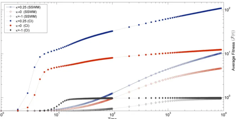
Besides the fitness increment at a fixed event of leader change, we also measured the fitness as a function of time as shown inFig 6. We observed that even though the fitness increases with time in all the three EVT domains, the rate at which the fitness increases depends strongly on the DBFE. This rate has an initial fast transient phase, after which it slows down.

The initial transient phase is strongly dependent on the initial condition as well as the muta-tion rate as shown inS2 Fig. The increase in fitness is fastest for the lowest initial condition, but it approaches the same fitness value as in the case of higher initial fitness in few generations. The time taken for populations of different initial fitness to reach the same fitness value depends on the mutation rate: forNμ1, it takes about 20 generations, whereas forNμ1,

Fig 6. Figure shows the average fitness increase with time for three different values ofκin the SSWM regime (Nμ= 0.01), and in the high mutation

regime(Nμ= 50).In all the cases, population starts with the same initial fitnessf0= 0.5.

it is approximately 200 generations. Even after this transient phase, the rate of increase in aver-age fitness (F_{ðtÞ) with time depends on the mutation rate as shown inFig 6. This is because of}

the fact that when a large number of mutations is available at the same time, a highlyfit mutant can invade the population and give a largefitness increment. Therefore, thefitness of a highly

fit mutant sequence would be greater in the high mutation regime compared to the one in a low mutation regime. The maximumfitness value reached in 9000 generations, in the case of Fréchet distribution, is about 10 times more for the high mutation regime, which is consistent with the expectation fromEq (7). Even beyond this point we noticed that thefitness is still increasing. In the same way, the Gumbel distribution also shows a significant increase in maxi-mumfitness reached in the high mutation regime as compared to the SSWM regime (about 4 times). Here also we found that thefitness is still increasing beyond the time point till which we tracked the dynamics. The bounded distribution (Weibull) reaches near the upper bound in SSWM and evolves slowly. However,fitness reaches afitness plateau in the high mutation regime and rate of adaptation becomes zero as can be seen inFig 6.

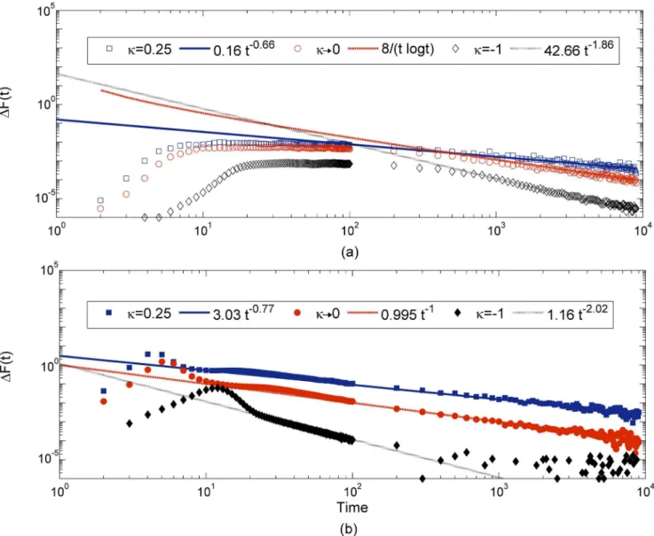
From this, we observe that the rate of change of fitness strongly depends on the properties of the underlying DBFE, which suggests that looking at this quantity can help us in distinguish-ing the DBFEs. Hence, we measured the fitness increment defined as

DF_{ðtÞ ¼ h}F_ðtþ1_Þ F_{ðtÞi; ð13Þ}

at each step. TheDF_{ðtÞinitially increases, then slowly decreases and settles down to a zero as}

shown inFig 7. If we denote this function as

DF_{ðtÞ ¼}A

ta; ð14Þ

whereAis a constant and the exponentαcan be used to distinguish the DBFE, since, as

explained below, exponentαis found to be greater (smaller) than one in the Weibull (Fréchet)

domain, but is close to one in the Gumbel domain.

In the SSWM regime, fromFig 7(a), we can see that each type of DBFE considered shows a different rate of decay. The Weibull domain has a faster decay withα= 1.86, the Gumbel

domain hasα1 [29] and the Fréchet domainα= 0.66 [29]. We observed that the same trend

is robust in a high mutation rate regime as well, whereαvalues are slightly larger in all cases. In

this regime alsoα= 2.02, 1 and 0.76 for the Weibull, Gumbel and Fréchet domains, respectively

as shown inFig 7(b). In the high mutation regime, in the case of Weibull distributions, fitness reaches a plateau in few generations, after which its rate of change goes to zero as observed in

Fig 7(b). The theoretical prediction for fitness at every time step for the unbounded distribu-tions belonging to the Gumbel and Frèchet domains was obtained by Park and Krug [29] in the low mutation regime. The comparison of our simulation data with these predictions shows a very good agreement in the Gumbel domain and in the Fréchet domain (up to a constant). In this work, we have also considered the bounded distribution and observed that its rate of decrease is faster with an exponent greater than one, which was not considered in the previous studies. We observed that even in a high mutation regime, the exponentαshows the same

behaviour. In this regime, the rate of change of fitness has been calculated only for exponential distribution belonging to the Gumbel domain [29] and their prediction matches with our data. In this work, we have obtained a complete picture by studying the rate of change of fitness numerically for the other two EVT domains as well.

Discussion

The main purpose of our work is to determine the quantities that can be used to distinguish the different extreme value domains of DBFE. Previous studies [16,18] have found that in an adapting population, the fitness gain at each fixation event shows qualitatively different trends in the three DBFE domains when the number of mutants produced in the population is much less than one at every generation (Nμ1). The focus of this work is to explore the parameter

regime in which the number of mutants produced is much above one (Nμ1). When the

mutation rate is high, the population becomes polymorphic and the better mutants existing in the population compete with each other. From our study, we have observed that the qualitative trends found for fitness difference when a new mutation establishes in the low mutation regime hold irrespective of the number of mutants produced. Thus, this study suggests that the

Fig 7. Figure shows the fitness increment in each time step for three different values ofκin two mutation regimes (SSWM and high mutation).In each case the data is fitted with the theoretically expected function given inEq (14), except for the exponential distribution for which we used the theoretical prediction by Park and Krug [29]. In all cases, the population starts with the same initial fitnessf0= 0.5.

fitness difference between successive mutations that spread in the population is a very impor-tant and robust quantity that can be used to predict the DBFEs in a more general scenario.

From our simulations, we see that as the initial fitness is increased, the fitness difference at the first step given byDfstepreduces, approaches a constant, or increases with the initialfitness in

the Weibull, Gumbel and Fréchet domains, respectively. We can understand these trends by a heuristic reasoning as discussed in detail in the Results section. This argument explains the increase inDfstepwithf0for an unbounded power law distribution and shows that the trends are determined by the behaviour of the tail (bounded/unbounded), and not by the details of the model.

Another important measure in understanding the dynamics of adaptation is the rate at which it occurs. Most of the previous studies which measured the adaptation rate have only considered exponentially distributed fitness distributions [20–22,28,34]. A previous study by Park and Krug [29] also considered DBFEs belonging to the Fréchet domain, but only in the SSWM regime (seeTable 1). In this work, we have extended the previous studies by numeri-cally measuring the rate of change of fitness for bounded distributions as well. We have mea-sured the rate of change of fitness in all the three EVT domains of the DBFE in both low and high mutation regimes. We observed that in all the cases, the rate of change of fitness decreases with time as*t−α

, whereα_>1 for Weibull,α1 for Gumbel [29] andα_<1 for Fréchet

domains [29].

Experimentally, the distribution of beneficial fitness effects can be inferred by two methods. In the first method, mutations are introduced in the wild type sequence and those that confer a fitness advantage are separated and their distribution of fitness effects are determined. In this method, DBFE belonging to all the EVT domains have been observed [5–14]. In contrast, here we focus on learning about DBFE via adaptation dynamics. Though many works have tracked the dynamics of the population during adaptation [7,35–38], in most of them only the selec-tion coefficient of the mutant fixed was measured. In our study, we have observed that the selection coefficient as given byEq (11)always decreases, with the increasing initial fitness or increasing steps as shown inS3 Fig. Hence, this quantity is not useful to distinguish between the EVT domains. However, from our study we observe that the fitness difference between steps shows different patterns depending on the EVT domain of the DBFEs in both the high and low mutation regimes and can be used to distinguish between the EVT domains.

In this work, we have numerically shown that the fitness returns in each EVT domain is very robust and holds good even when the number of mutations produced is large (Nμ1).

Fitness difference can be measured in experiments, for example as in [5]. We suggest that experiments can predict the EVT domain of DBFE by measuring the fitness difference between successive mutations fixed in the population or even from the fitness of the first mutation, when the initial fitness is varied. However, currently experimental studies that measure both fitness and DBFE in the same study are not available, but it is highly desirable to have such studies to test our predictions.

Supporting Information

S1 Fig. The plot shows the fitness difference at the first step as a function of the initial fit-ness for differentκand two differentN_{μ.The lines give the theoretical values while the open} symbols are the simulation output forNμ= 0.02 and the closed symbols are those forNμ= 5.

(TIF)

S2 Fig. The figure shows the average fitness of the population for variousκin both the low

(closed symbols) are considered. (TIF)

S3 Fig. The main figure shows the selection coefficient as a function of step for all three

κvalues.We considered two differentNμwhere open symbols and closed symbols are for Nμ= 0.01 andNμ= 50, respectively. The inset shows the selection coefficient of various steps

for two different initial fitnessesf0= 0.2fmaxandf0= 0.6fmax, wherefmaxis calculated usingEq (7)in the high mutation regime.

(TIF)

Acknowledgments

We thank K. Jain for many useful discussions that helped us in this work and suggesting the heuristic argument discussed in the section‘Fitness and fitness difference’. We also thank J. Krug for bringing references [12,13] to our attention. We thank V. Yalasi for helping us to improve the figure quality.

Author Contributions

Conceived and designed the experiments: SJ SS. Performed the experiments: SJ SS. Analyzed the data: SJ SS. Contributed reagents/materials/analysis tools: SJ SS. Wrote the paper: SS SJ.

References

1. Bull JJ, Otto SP (2005) The first steps in adaptive evolution. Nat Genet 37: 342–343. doi:10.1038/

ng0405-342PMID:15800646

2. Eyre-Walker A, Keightley P (2007) The distribution of fitness effects of new mutations. Nat Rev Genet 8: 610. doi:10.1038/nrg2146PMID:17637733

3. Gillespie JH (1983) A simple stochastic gene substitution process. Theor Popul Biol 23: 202–215. doi:

10.1016/0040-5809(83)90014-XPMID:6612632

4. Sornette D (2000) Critical Phenomena in Natural Sciences. Springer, Berlin.

5. MacLean RC, Buckling A (2009) The distribution of fitness effects of beneficial mutations in Pseudomo-nas aeruginosa. PLoS Genetics 5: e1000406. doi:10.1371/journal.pgen.1000406PMID:19266075

6. Sanjuán R, Moya A, Elena S (2004) The distribution of fitness effects caused by single-nucleotide sub-stitutions in an RNA virus. Proc Natl Acad Sci USA 101: 8396–8401. doi:10.1073/pnas.0400146101

PMID:15159545

7. Rokyta D, Joyce P, Caudle S, Wichman H (2005) An empirical test of the mutational landscape model of adaptation using a single-stranded DNA virus. Nat Genet 37: 441–444. doi:10.1038/ng1535PMID:

15778707

8. Kassen R, Bataillon T (2006) Distribution of fitness effects among beneficial mutations before selection in experimental populations of bacteria. Nat Genet 38: 484–488. doi:10.1038/ng1751PMID:

16550173

9. Rokyta DR, Beisel CJ, Joyce P, Ferris MT, Burch CL, et al. (2008) Beneficial fitness effects are not exponential for two viruses. J Mol Evol 69: 229.

10. Bataillon T, Zhang T, Kassen R (2011) Cost of adaptation and fitness effects of beneficial mutations in Pseudomonas fluorescens. Genetics 189: 939–949. doi:10.1534/genetics.111.130468PMID:

21868607

11. Schenk MF, Szendro IG, Krug J, de Visser JAGM (2012) Quantifying the adaptive potential of an antibi-otic resistance enzyme. PLoS Genet 8: e1002783. doi:10.1371/journal.pgen.1002783PMID: 22761587

12. Foll M, Poh YP, Renzette N, Ferrer-Admetlla A, Bank C, et al. (2014) Influenza virus drug resistance: A time-sampled population genetics perspective. PLoS Genet 10(2). doi:10.1371/journal.pgen.1004185 PMID:24586206

14. Rokyta DR, Abdo Z, Wichman HA (2009) The genetics of adaptation for eight microvirid bacterio-phages. J Mol Evol 69: 229. doi:10.1007/s00239-009-9267-9PMID:19693424

15. Jain K, Seetharaman S (2011) Multiple adaptive substitutions during evolution in novel environments. Genetics 189: 1029–1043. doi:10.1534/genetics.111.134163PMID:21900275

16. Seetharaman S, Jain K (2014) Adaptive walks and distribution of beneficial fitness effects. Evolution 68: 965–975. doi:10.1111/evo.12327PMID:24274696

17. Seetharaman S, Jain K (2014) Length of adaptive walk on uncorrelated and correlated fitness land-scapes. Phys Rev E 90: 32703. doi:10.1103/PhysRevE.90.032703

18. Seetharaman S (2011) Adaptation on rugged fitness landscapes. M. S. thesis, JNCASR, Bangalore.

19. Muller HJ (1964) The relation of recombination to mutational advance. Mutation Res 1: 2–9. doi:10.

1016/0027-5107(64)90047-8

20. Gerrish PJ, Lenski RE (1998) The fate of competing beneficial mutations in an asexual populations. Genetica 102: 127–144. doi:10.1023/A:1017067816551PMID:9720276

21. Park SC, Krug J (2007) Clonal interference in large populations. PNAS 104: 18135–18140. doi:10.

1073/pnas.0705778104PMID:17984061

22. Desai M, Fisher D (2007) Beneficial mutation-selection balance and the effect of linkage on positive selection. Genetics 176: 1759–1798. doi:10.1534/genetics.106.067678PMID:17483432

23. Jain K, Krug J, Park SC (2011) Evolutionary advantage of small populations on complex fitness land-scapes. Evolution 65–7: 1945–1955. doi:10.1111/j.1558-5646.2011.01280.x

24. de Visser JAGM, Rozen DE (2006) Clonal interference and the periodic selection of new beneficial mutations in escherichia coli. Genetics 172: 2093–2100. doi:10.1534/genetics.105.052373PMID:

16489229

25. de Visser JAGM, Zeyl C, Gerrish P, Blanchard J, Lenski R (1999) Diminishing returns from mutation supply rate in asexual populations. Science 283: 404–406. doi:10.1126/science.283.5400.404 26. Miralles R, Gerrish PJ, Moya A, Elena S (1999) Clonal interference and the evolution of rna viruses.

Sci-ence 285: 813–815. doi:10.1126/science.285.5434.1745

27. Rozen D, de Visser JAGM, Gerrish PJ (2002) Fitness effects of fixed beneficial mutations in microbial populations. Curr Biol 12: 1040–1045. doi:10.1016/S0960-9822(02)00896-5PMID:12123580 28. Park SC, Simon D, Krug J (2010) The speed of evolution in large asexual populations. J Stat Phys 138:

381–410. doi:10.1007/s10955-009-9915-x

29. Park SC, Krug J (2008) Evolution in random fitness landscapes: the infinite sites model. J Stat Mech: Theor Exp 2008: P04014. doi:10.1088/1742-5468/2008/04/P04014

30. Wilke C, Martinetz T (1999) Adaptive walks on time-dependent fitness landscapes. Phys Rev E 60: 2154–2159. doi:10.1103/PhysRevE.60.2154

31. Orr HA (2003) The distribution of fitness effects among beneficial mutations. Genetics 163: 1519–

1526. PMID:12702694

32. Rosenberg N (2005) A sharp minimum on the mean number of steps taken in adaptive walks. J theor Biol 237: 17–22. doi:10.1016/j.jtbi.2005.03.026PMID:15979094

33. Kryazhimskiy S, Tkačik G, Plotkin JB (2009) The dynamics of adaptation on correlated fitness land-scapes. Proc Natl Acad Sci USA 106: 18638–18643. doi:10.1073/pnas.0905497106PMID:19858497 34. Campos P, Wahl LM (2010) The adaptation rate of asexuals: deleterious mutations, clonal interference

and population bottlemecks. Evolution 64(7): 1973–1983. PMID:20199567

35. Schoustra S, Bataillon T, Gifford D, Kassen R (2009) The properties of adaptive walks in evolving popu-lations of fungus. PLoS Biol 7 (11): e1000250. doi:10.1371/journal.pbio.1000250PMID:19956798

36. MacLean RC, Perron GG, Gardner A (2010) Diminishing returns from beneficial mutations and perva-sive epistasis shape the fitness landscape for rifampicin resistance inPseudomonas aeruginosa. Genetics 186: 1345–1354. doi:10.1534/genetics.110.123083PMID:20876562

37. Gifford DR, Schoustra SE, Kassen R (2011) The length of adaptive walks is insensitive to starting fit-ness inAspergillus nidulans. Evolution 65: 3070–3078. doi:10.1111/j.1558-5646.2011.01380.xPMID:

22023575