ISSN 0101-8205 / ISSN 1807-0302 (Online) www.scielo.br/cam
Numerical solution of coupled mass and energy
balances during osmotic microwave dehydration
JAVIER R. ARBALLO1,2∗
, LAURA A. CAMPAÑONE1,2
and RODOLFO H. MASCHERONI1,2
1CIDCA (Centro de Investigación y Desarrollo en Criotecnología de Alimentos) (CONICET La Plata – UNLP), Calle 47 y 116, La Plata (1900), Argentina 2MODIAL – Facultad de Ingeniería, Universidad Nacional de la Plata (UNLP) E-mails: [email protected] / [email protected] / [email protected]
Abstract. The mass and energy transfer during osmotic microwave drying (OD-MWD) pro-cess was studied theoretically by modeling and numerical simulation. With the aim to describe the transport phenomena that occurs during the combined dehydration process, the mass and energy microscopic balances were solved. An osmotic-diffusional model was used for osmotic dehydration (OD). On the other hand, the microwave drying (MWD) was modeled solving the mass and heat balances, using properties as function of temperature, moisture and soluble solids content. The obtained balances form highly coupled non-linear differential equations that were solved applying numerical methods. For osmotic dehydration, the mass balances formed coupled ordinary differential equations that were solved using the Fourth-order Runge Kutta method. In the case of microwave drying, the balances constituted partial differential equations, which were solved through Crank-Nicolson implicit finite differences method. The numerical methods were coded in Matlab 7.2 (Mathworks, Natick, MA). The developed mathematical model allows predict the temperature and moisture evolution through the combined dehydration process.
Mathematical subject classification: Primary: 06B10; Secondary: 06D05.
Key words:mathematical modeling, osmotic-microwave, combined dehydration.
1 Introduction
Osmotic dehydration (OD) has the ability to protect the food for further drying treatments, as it generates a defense from losses in volatile compounds and lowers the risks of chemical and physical changes. It consists in food immersion in a hypertonic solution that produces a partial water removal. To complete the drying process and reach a stable product it is necessary another procedure like microwave drying (MWD). Microwaves have the ability to penetrate and heat within products, due to the interaction of the electric field with water molecules. When using microwave as a final drying stage, the removing of inner water is enhanced because foods heat uniformly increasing water vapor pressure which forces vapor toward the surface [1].
There exist mathematical models to describe the mass transfer process during osmotic dehydration that cover a wide range of approaches and forms. According to Spiazzi and Mascheroni [2] the OD models could be divided into two main groups: the phenomenological and microscopic-structural ones. In the present work osmotic diffusional model developed by Spiazzi and Mascheroni [3], based on the research works of Toupin et al. [4] and Marcotte et al. [5], was used to model osmotic dehydration process, which is based on the mass transfer through cellular membranes and multicomponent diffusion between intercellular spaces. Besides, the electromagnetic-food interaction has to be considered in the model formulation. The behavior of the electromagnetic field inside the microwave oven is very complex; then it can be used an approximation that considers an exponential decay inside the food, the Lambert’s law [6, 7].
To model the combined process of osmotic dehydration followed by microwave drying it is necessary to solve the microscopic mass and energy balances. The obtained balances constitute a system of nonlinear differential equations highly coupled. For osmotic dehydration process, the mass balances constitute ordinary coupled differential equations; in the case of microwave drying the balances constitute partial differential equations. For the characteristics of the equation system, it should be solved applying numerical methods.
According of the previous considerations the objectives of this work were:
– To solve the non-linear mathematical model considering that the thermal, electromagnetic and transport properties are temperature and composition dependent.
– To apply the developed model to simulate the mass and temperature profiles under different operating conditions.
2 Mathematical Modeling
In the development of the mathematical model two fundamentals steps have been considered: osmotic dehydration process and the application of microwave as a final drying step.
2.1 Osmotic dehydration (Step 1)
In this step Spiazzi and Mascheroni [3] model was used, that considers the mass transfer through cellular membranes and the multicomponent diffusion between intercellular spaces. In order to obtain the concentration profiles, the whole vol-ume was divided intoNconcentric and equal volume shells. In each element two phases may be distinguished: the plasmatic content and the intercellular spaces. Each volume of intercellular space is subjected to a diffusive-convective flux between adjacent volumes and a transmembrane diffusive flux from the cellular plasma [3]. The mass balances for each volumeVξ(ξ =1,N)are presented as follows:
d Mj,c dt
= −nj,c.Ac (1)
nj,c
=kwc1(cj,c)c−o (2)
d Mj,o dt
=1(nj,o.Ao)+nj,c.Ac (3)
nj,o
= Dj.∇(cj,o)+cj,o.u (4)
whereM,n andcare the mass, flux and concentration of the j specie,
respec-tively. The subscriptsc ando indicate cellular and extracellular space; D and
areas andz represents the distance between each volume element Vξ. 1(cj,c)
indicates the concentration difference between intra and extra cellular spaces of the component j and∇(cj,o)is the concentration gradient between adjacent
volume elements.
The model considers the shrinkage rateu, which can be calculated from the
following relation:
u = d z
dt (5)
The cellular and extracellular transfer areas can be calculated as follows:
Ac =Ncell.Vc2/3 (6) Ac =Cg.Vo2/3.e (7)
where Ncell andCg are constants which depend on the cell shape, the number
of cells per unit volume and the shape of the product piece; Vc andVoare the
cellular and extracellular volume;erepresents the fraction of the geometric area
which belongs to the extracellular spaces.
The concentration values in the hypertonic solution are deduced from the total mass balances:
N
X
ξ=1 (Mξj,o)
dt = −
(Mosmj,sol)
dt (8)
whereMξj,ocorresponds to the mass of component jinside the osmotic solution and subscript sol indicates osmotic solution.
2.2 Microwave dehydration (Step 2)
In the final drying step two stages must be considered: stage 2.1 – Heating with weak evaporation and stage 2.2 – Intensive evaporation. Besides, the fol-lowing assumptions were made when developing the microwave mathematical model [8]:
– Uniform initial temperature and water content within the product,
– Temperature – and moisture content-dependent dielectric properties,
– Volume changes are not considered,
– Regular one-dimensional geometry (1D),
– Uniform electric field distribution around the sample, and a dominant polarization of the electric field normal to the surface.
2.2.1 Microwave heating
The stage 2.1 involves the heating of the food up to the moment when the whole product reaches the equilibrium temperature Teq. To describe heat transfer, an energy balance must be developed that considers a source term of internal heat generation due to the energy supplied by MW [9]. The resulting microscopic energy balance can be expressed in terms of power as [10]:
VρCp ∂T
∂t =V(∇k∇T)+P (9)
where V is product volume, ρ is density, C p specific heat capacity, T tem-perature, t time, k thermal conductivity and P is the power generated by
the absorption of microwaves. Fresh food physical properties are used in equation 9.
To complete the model, the following initial and boundary conditions are considered:
T =0 T =Ti ni 0≤x ≤2L (10)
x =0,2L −k∂T
∂x =h(T −Ta)+Lvap km(Cw−Ceq) t>0 (11)
where L is the half thickness, Ti ni is initial temperature,h is the heat transfer
coefficient, Ta is the environment temperature, Lvap is the water heat
vapor-ization,km is the mass transfer coefficients, Cw andCeq are the moisture and
equilibrium concentrations. Equation 11 includes vaporization at the food sur-face. This assumption is valid only for the heating step because the exposure time is short and the product temperature over this period is below Teq. In this step, it could be assumed that weak evaporation occurs and equation 11 can be applied. Other authors also used this boundary condition in microwave heating processes, when modeling the initial heating step [6, 11, 12]. A value of 5 (W m−2 C−1) was employed for natural convection around the product
JH = JDallowed to estimatekmfromhvalues [13]. The power absorbed during
microwave irradiation on both sides is represented by the term P. Heat
genera-tion is a funcgenera-tion of the temperature in each point of the material. In this work, Lambert’s Law is deemed as valid.
P = PRi+Le =P′(e
−2α(L−x)+e−2α(x))
o (12)
α= 2π
λ
s
ǫ[(1+tan2δ)2−1]
2 (13)
δ=tan−1(ǫ′′/ǫ′)) (14)
whereP′
ois the incident power at the surface (W),Ri andLeindicate right and
left sides,λis the wavelength of radiation andαis the attenuation factor, which is a function of the dielectric constantǫ′and of the loss factorǫ′′.
To predict the humidity profile during the heating stage, a microscopic balance of mass is needed that considers the water diffusion in the inner part of the food. This balance is:
∂Cw
∂t = ∇(Dw∇Cw) (15)
The following initial and boundary conditions are considered:
t=0 Cw =Cw,i ni 0≤ x ≤2L (16)
x =0,2L −Dw
∂Cw
∂x =kw(Cw−Ceq) t>0 (17)
2.2.2 Microwave intensive vaporization
The stage 2.2 of microwave drying takes place when the whole product reaches
Teq and intensive evaporation begins. Teq is the temperature achieved when the
power absorbed is equilibrated with the energy used in water vaporization [8]. This step finishes at the end of the constant temperature period, unless there is a requirement to heat the material after it is dried. In the energy transfer step, the temperature is supposed to be at the equilibrium value in whole the foodTeq.
Then Lambert’s law was applied to evaluate the distribution of electromagnetic energy inside the food. The following equation was applied:
P= PRi+Le = P′(e
−2αd(L−x)+e−2αd(x))
o (19)
whereαd is the attenuation factor calculated using dielectric properties of the
dehydrated material.
The model takes into account the continuous or intermittent application of MW power considering null the incident microwave power when the magnetron is turned off in the cycling operation mode.
During this final stage, water vaporization is considered to take place vol-umetrically within the product. The generation of water vapor is calculated supposing that all the power generated by MW is used for removal of water:
mvLvap =
Z V
0
Qd V (20)
wheremvis the rate of water vaporization (kg s−1).
3 Results
3.1 Numerical solution
3.1.1 Osmotic dehydration model (step 1)
In this step the model solves 2N equations for water (j =w) andN equations
for soluble solids content (j =s), in order to calculate water and soluble solids
content inside the food. The obtained ordinary differential equation system can be solved through Fourth Order Runge-Kutta method coded in Matlab 7.2 (Mathworks, Natick, MA). The domain was divided into 10 volume elements and the equations 21-39 were solved for each volume and time increment (1t):
Cell volume
d(Mξj,c)
dt =
d(cξj,cVξ c)
dt = f(t,cj,c) (21)
f(t,cj,c)= −kwc.1(cξj,c)c,o.Aξc (22)
1(cξj,c)c,o=(c ξ
j,c−c ξ
kξR K1= f(t,cξj,c) (24) kξR K2= f(t+1t/2,cξj,c+kξR K11t/2) (25) kξR K3= f(t+1t/2,cξj,c+kξR K21t/2) (26)
kξR K4= f(t+1t,cξj,c+kξR K31t) (27)
kξR K T =1/6(kξR K1+2kξR K2+2kξR K3+kξR K4) (28) Mξj,c;t+1t =Mξj,c;t +kξR K T1t (29)
Intercellular volume
d(Mξj,o)
dt =
d(cξj,oVoξ)
dt =g(t,cj,o) (30)
g(t,cj,o)=1[(Dj.∇(c ξ
j,o)c,o+c ξ
j,o.u ξ).Aξ
o] ξ,ξ+1
+(kwc.1(c ξ
j,c)c,o).Aξc (31)
∇(cξj,o)c,o=
(cξj,+1o −cξj,o)
1zξ (32)
uξ = z
ξ+1−zξ
dt (33)
mξR K1=g(t,cξj,o) (34) mξR K2=g(t+1t/2,cξj,o+mξR K11t/2) (35)
mξR K3=g(t+1t/2,cξj,o+mξR K21t/2) (36)
mξR K4=g(t+1t,cξj,o+mξR K31t) (37) mξR K T =1/6(mξR K1+2mξR K2+2mξR K3+mξR K4) (38) Mξj,o;t+1t =Mξj,o;t +mξR K T1t (39)
where1t is the time increment (0.1s for all the runs), f(t,cj,c)andg(t,cj,o)
correspond to mass variation of the j component with respect to time, inside
the cell (subscript c) and between adjacent intercellular spaces (subscript o); Mξj,c;t+1t and M
ξ
j,o;t+1t are the new values of mass of water or solids at time t+1t, in the cellular and extracellular volume, respectively;kR K andmR K are
3.1.2 Microwave drying model (steps 2)
The mass and energy balances in the stage 2.1 with their boundary conditions are coupled and form a system of nonlinear partial differential equations. There-fore, Crank-Nicolson finite difference method, characterized by being uncondi-tionally stable and convergent, was used for solving the final equation system. A finite difference algorithm, previously developed by Campañone et al. [16], was implemented to solve the unidirectional energy transfer. A time increment of 0.1s was used and the domain was divided into 15 space increments. The following equations were obtained for the inner points to calculate the tempera-ture profiles.
Tin+1+1
− Vik
n i
21x2−
Vi(kin+1−kin−1)
81x2
+Tin+1
ViρinC pni
1t +
Vikin 1x2
+Tin−1+1
− Vik
n i
21x2 +
Vi(kin+1−kni−1)
81x2
=Tin+1
Vikin
21x2 +
Vi(kni+1−kni−1)
81x2
+Tin
ViρinC pin
1t −
Vikin 1x2
+Tin−1
Vikin
21x2−
Vi(kin+1−kin−1)
81x2
+Pi
(40)
This equation is valid for 0 < i < b being b the number of nodes in the discretized domain. V i is the volume of an element located between the nodes
(i+1/2)and(i−1/2), and Pi is the power calculated in the same nodes:
Pi =Po Ai nc
At
e−2α(L−(i+1/2)1x)−e−2α(L−(i−1/2)1x) (41)
At the food surface(i =b), equation 40 presents two fictitious points(i+1,n)
and(i+1,n+1). Using boundary condition equation 11, the following equations
were obtained:
Tin+1,f =Tin−1− 21x
kin hT n
i +
21x
kin hTa (42)
Tin+1+1,f =Tin−1+1−21x
kin hT n+1
i +
21x
By replacing equation 42 and 43 in the general expression equation 40, the temperature prediction equation was:
Tbn+1
VbρbnC pbn
1t +
Vbknb 1x2 +
2Vbh1x kn
b
kn b
21x2 + kn
b+1−knb−1
81x2
+Tbn−1+1
−Vbknb
1x2
=Tbn
VbρbnC pnb
1t −
Vbkbn 1x2 +
2Vbh1x kn b − k n b
21x2 − kn
b+1−kbn−1
81x2
+Tbn−1
V
bkbn 1x2
+2Vbh1x Ta
knb
kn b
21x2 +
knb+1−knb−1
81x2
+Pb
(44)
Equations 40 and 44 for both boundaries, form a system of linear equations. The solution allows calculate the inner and surface temperatures. The same procedure was implemented to solve the microscopic mass balance equations 15-17. In stage 2.2, moisture content for each time step was calculated using equation 20.
The equation system solution to obtain temperatures and moisture profiles were coded in Matlab 7.2 (Mathworks, Natick, MA).
3.2 Process simulation
The mathematical model can be used for a wide variety of food materials. Firstly, the model was employed to predict the water loss and solid gain during OD process (Step 1) applied to pumpkin in sucrose solution.
Table 1 summarizes the physical properties and adjustment parameters needed to run the simulation.
In this Table the subscript 60 indicates the concentration of osmotic solution (Brix units). In Figures 1a and b it can be seen the experimental and simulated values of water loss and solid gain. The model follows the experimental behavior; a rapid increase in the first 300 minutes, and from then a trend to equilibrium.
Property Value Note
Food pumpkin Experimental data from Arballo et al. [17]
shape slice −
kw(m s−1) 220 10−9 Mass transfer coefficient (water)
DW60(m2s−1) 2.12 10−9 Diffusion coefficient at 60Bx (water)
DS60(m2s−1) 0.25 10−9 Diffusion coefficient at 60Bx (sucrose)
Sample thickness(m) 0.010 −
Sample diameter(m) 0.031 −
Table 1 – Parameters, transport and diffusional properties of pumpkin for OD-model simulation.
Property Value Note
Food pear Experimental data from Arballo et al. [17]
shape half slice −
kw(m s−1) 200 10−9[18] Mass transfer coefficient
DW 60(m2s−1) 1.36 10−9 Diffusion coefficient at 60Bx (water)
DS60(m2s−1) 0.17 10−9 Diffusion coefficient at 60Bx (sucrose)
DW 40(m2s−1) 1.07 10−9 Diffusion coefficient at 40Bx (water)
DS40(m2s−1) 0.23 10−9 Diffusion coefficient at 40Bx (sucrose)
DW 20(m2s−1) 4.08 10−9 Diffusion coefficient at 20Bx (water)
DS20(m2s−1) 1.02 10−9 Diffusion coefficient at 20Bx (sucrose)
Sample thickness(m) 0.010 −
Sample diameter(m) 0.052 −
Table 2 – Parameters, transport and diffusional properties of pear for OD-model simulation.
Figure 2 – Simulated (lines) and experimental (symbols) water loss during osmotic de-hydration process applied for three different solution concentrations to pear half slices.
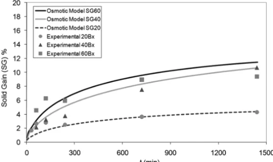
Figure 3 – Simulated (lines) and experimental (symbol) solid gain during osmotic de-hydration process applied for three different solution concentrations for pear half slice.
more water content reduction and gained more solids than pears; it corresponds to the different values of the Dw and Ds parameters for the two foods, and is based mainly in differences in structure.
Besides, the mathematical model also considered the variation of OD solution concentration, shape and size of the product.
With respect to OD solution concentration, the experimental values for pear fruit ranged between 20 to 60 Brix. The model is sensible to the change of solution composition as can be seen in Figures 2 and 3, showing a good accuracy in the predicted curves as compared to experimental data.
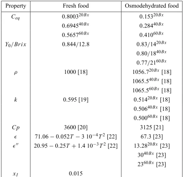
For Step 2 (MWD), Table 3 shows the thermal, transport and electromagnetic properties used as inputs in the runs of the numerical model.
The model allows predict the evolution of temperature and moisture content during step 2 (Figs. 4 and 5). OD process applied to pears in sucrose solution during two hours was considered as initial condition for this stage. Different OD pre treatments affect the initial water and solute content. The model takes into account this fact varying moisture and solid content of the food (Fig. 4).
Property Fresh food Osmodehydrated food
Ceq 0.800320Bx 0.15320Bx
0.694540Bx 0.28440Bx
0.565760Bx 0.41060Bx Y0/Br i x 0.844/12.8 0.83/1420Bx
0.80/1840Bx
0.77/2160Bx
ρ 1000 [18] 1056.720Bx[18]
1065.540Bx[18]
1065.560Bx[18]
k 0.595 [19] 0.51420Bx [18]
0.50640Bx [18]
0.50060Bx [18]
C p 3600 [20] 3125 [21]
ǫ 71.06−0.052T−3 10−4T2[22] 67.3 [23] ǫ′′ 20.95−0.25T +1.4 10−3T2[22] 13.2820Bx [23]
3040Bx[23]
2360Bx [23]
xI 0.015
Table 3 – Thermal, transport and electromagnetic properties of food for model simulation.
The microwave oven operates in continuous or intermittent modes, according to power used. The dehydration process of fruits and vegetables can be enhanced applying on-off cycles (Campañone et al. [24]). The model was able to follow the intermittency of microwave power application (on-off operation), being sta-ble and showing no perturbations in the predicted temperature and moisture profiles (Fig. 5).
Figure 4 – Predicted moisture content as a function of time for different osmotic pre-treatments (20, 40 and 60 Brix) when applying microwave power of 500W.
Figure 5 – Predicted temperatures as a function of time for different osmotic pretreat-ments (20, 40 and 60 Brix) when applying microwave power of 500W.
Figure 6 – Simulated thermal histories (surface) applying different microwave power levels.
Figure 8 – Simulated moisture contents applying different microwave power levels.
4 Conclusions
A complete and relatively simple and easy to use mathematical model has been developed for simultaneous prediction of temperature and moisture profiles dur-ing the combined process of osmotic-microwave dehydration. Its main original-ity is that it can consider the initial process of osmotic dehydration and couple the predicted water and solute concentration profiles to the simultaneous mass and energy transfer in the microwave heating step including, also, the inner heat generation, the on-off control effect of the microwave oven and different power levels. The model considers two numerical techniques to solve differential equa-tions: Runge Kutta (fourth order) for Step 1 and Finite Differences for Step 2. The numerical solution of the balances was implemented in Matlab environment and it permits to interpret and simulate a technological and industrial process.
Figure 9 – Simulated temperature (a) and moisture contents (b) during MWD for dif-ferent sample thicknesses.
REFERENCES
[1] A.K. Datta and J. Zhang, Porous media approach to heat and mass transfer in solid foods. Department of Agriculture And Biology Engineering, Cornell
Uni-versity (1999).
[2] E.A. Spiazzi and R.H. Mascheroni, Modelo de deshidratación osmótica de alimentos vegetales. MAT Serie A,4(2001), 23–32.
[3] E.A. Spiazzi and R.H. Mascheroni, Mass transfer model for osmotic dehydration of fruits and vegetables. I. Development of the simulation model. Journal of Food Engineering,34(1997), 387–410.
[4] C.J. Toupin, M. Marcotte and M. Le Maguer, Osmotically induced mass trans-fer in plant storage tissues: a mathematical model – Part I. Journal of Food Engineering,10(1989), 13–38.
[5] M. Marcotte, C.J. Toupin and M. Le Maguer, Mass transfer in cellular tissues. Part I: The mathematical model. Journal of Food Engineering,13(1991), 199–
220.
[6] C.H. Tong and D.B. Lund, Microwave heating of baked dough products with simultaneous heat and moisture transfer. Journal of Food Engineering,19(1993),
319–339.
[7] H. Ni and A.K. Datta, Moisture as related to heating uniformity in microwave processing of solids foods. Journal of Food Process Engineering,22(2002), 367–
382.
[8] J.R. Arballo, L.A. Campañone and R.H. Mascheroni, Modelling of microwave drying of fruits. Drying Technology,28(2010), 1178–1184.
[9] Y.E. Lin, R.C. Anantheswaran and V.M. Puri, Finite element analysis of micro-wave heating of solid foods. Journal of Food Engineering,25(1995), 85–112. [10] L.A. Campañone and N.E. Zaritzky, Mathematical analysis of microwave
heat-ing process. Journal of Food Engineering,69(2005), 359–368.
[11] L. Zhou, V.M. Puri, R.C. Anantheswaran and G. Yeh, Finite element modelling of heat and mass transfer in food materials during microwave heating-model, development and validation. Journal of Food Engineering,25(1995), 509–529.
[12] M. Pauli, T. Kayser, G. Adamiuk and W. Wiesbeck,Modeling of mutual coupling between electromagnetic and thermal fields in microwave heating. IEEE,2007
[13] R.B. Bird, W.E. Stewart and E.N. Lightfoot, Transport phenomena. John Wiley and Sons, New York (1976).
[14] A. Constantinides and N. Mostoufi,Numerical Methods for Chemical Engineers with Matlab Applications. Prentice-Hall (1999).
[15] S.C. Chapra and P.P. Canale,Métodos Numéricos para Ingenieros. Fifth Edition.
México, Mc Graw-Hill (2007).
[16] L.A. Campañone, V.O. Salvadori and R.H. Mascheroni, Weight loss during freezing and storage of unpackaged foods. Journal of Food Engineering,47(2001),
69–79.
[17] J.A. Arballo, R.R. Bambicha, L.A. Campañone, M.E. Agnelli and R.H. Masche-roni, Mass transfer kinetics and regressional-desirability optimization during osmotic dehydration of pumpkin, kiwi and pear. International Journal of Food
Science and Technology,47(2012), 306–314.
[18] M.E. Agnelli, C.M. Marani and R.H. Mascheroni, Modelling of heat and mass transfer during (osmo) dehydrofreezing of fruits. Journal of Food Engineering,69
(2005), 415–424.
[19] V.E. Sweat, Experimental values of thermal conductivity of selected fruits and vegetables. Journal of Food Science,39(1974), 1080–1083.
[20] S.L. Polley, O.P. Snyder and P. Kotnour,A compilation for thermal properties of foods. Food Technology,34(1980), 76–94.
[21] A.M. Tocci and R.H. Mascheroni,Determinación por calorimetría diferencial de barrido de la capacidad calorífica y entalpía de frutas parcialmente deshidratadas en soluciones acuosas concentradas de azúcar. In: I Congreso Ibero-Americano de Ingeniería de Alimentos,I(1996), 411–420.
[22] O. Sipahioglu and S.A. Barringer, Dielectric properties of vegetables and fruits as a function of temperature, ash and moisture content. Journal of Food Science,
68(2003), 234–239.
[23] A.K. Datta and R.C. Anantheswaran, Handbook of Microwave Technology for Food Applications. Marcel Dekker, USA (2001).