Copyright © 2012 SBMAC
ISSN 0101-8205 / ISSN 1807-0302 (Online) www.scielo.br/cam
Ostrowski type inequalities for interval-valued
functions using generalized Hukuhara derivative
∗Y. CHALCO-CANO, A. FLORES-FRANULI ˇC and H. ROMÁN-FLORES Instituto de Alta Investigación, Universidad de Tarapacá, Casilla 7D, Arica-Chile
E-mails: [email protected] / [email protected] / [email protected]
Abstract. The present paper is devoted to obtaining some Ostrowski type inequalities for valued functions. In this context we use the generalized Hukuhara derivative for interval-valued functions. Also some examples and consequences are presented.
Mathematical subject classification: Primary: 26E25; Secondary: 35A23.
Key words: Ostrowski type inequalities, interval-valued functions,g H-differentiability and integrability of interval-valued functions.
1 Introduction
The importance of the study of set-valued analysis from a theoretical point of view as well as from their application is well known [5, 7]. Many advances in set-valued analysis have been motivated by control theory and dynamical games [6]. Optimal control theory and mathematical programming were a motivating force behind set-valued analysis since the sixties [6]. Interval Analysis is a particular case and it was introduced as an attempt to handle interval uncertainty that appears in many mathematical or computer models of some deterministic real-world phenomena. The first monograph dealing with interval analysis was given by Moore [14]. Moore is recognized to be the first to use intervals in computational
#CAM-430/11. Received: 14/X/11. Accepted: 06/V/12.
mathematics, now called numerical analysis. He also extended and implemented the arithmetic of intervals to computers. One of his major achievements was to show that Taylor series methods for solving differential equations not only are more tractable, but also more accurate [15].
The following inequality is known in the literature as Ostrowski’s inequality
1
b−a Z b
a
f(y)dy− f(x)
≤ 1
4 +
x− a+b2 2
(b−a)2
!
(b−a)f′
∞, (1)
where f ∈C1([a,b]),x ∈ [a,b]. Inequality (1) is sharp, see [3]. Since 1938 when A. Ostrowski (see [16]) presented his famous inequality many researchers have been working about and around it, in many different directions and with a lot of applications. In the book edited by Dragomir and Rassias [11] and recently in the book of Anastassiou [1] are given a brief review of state of art about Ostrowski type inequalities and its applications.
Continuing that tradition, in [2] the Ostrowski type inequality has been ex-tended to context of fuzzy-valued functions. In this context has been used the concept of Hukuhara-derivative for fuzzy-valued functions. Note that interval-valued functions are fuzzy-interval-valued functions. Thus, the fuzzy Ostrowski type inequalities obtained in [2] is valid for interval-valued functions. However, the concept ofH-derivative for interval-valued functions is very restrictive, see [8, 9]. Generalized Hukuhara differentibility it is the most general differentiability concept for interval-valued functions, see [8, 9, 19].
Motivated by [1, 2, 3, 11] and [8, 9, 13, 19] we extend Ostrowski type inequal-ity (1) forg H-differentiable interval-valued functions.
2 Basic concepts
LetRbe the one-dimensional Euclidean space. Following [10], letKC denote the family of all non-empty compact convex subsets ofR, that is,
KC = {[a,b] |a,b ∈R and a ≤b}.
The Hausdorff metric HonKC is defined by
where
d(A,B)=max
a∈A d(a,B) and d(a,B)=minb∈Bd(a,b)=minb∈B |a−b|. It is well known that (KC,H)is a complete metric space (see [5, 10]). The Minkowski sum and scalar multiplication are defined by
A+B = {a+b|a ∈ A, b∈ B} and λA= {λa|a ∈ A}. (2)
The spaceKC is not a linear space since it does not possess an additive inverse and therefore subtraction is not well defined (see [5, 9, 10, 19]). Actually,KC is a quasilinear space [4, 17].
A crucial concept in obtaining a useful working definition of derivative for interval-valued functions is considering a suitable difference between two inter-vals. Toward this end, one way is to use (2) by requiring
A−B = A+(−1)B.
However, this definition of difference has the drawback that
A−A6= {0} (3)
in general (the exception is when we have a zero width interval, A= [a,a], that is, a real number). One of the first attempts to overcome (3) was due to Hukuhara [12] who defined what has become to be known as the Hukuhara difference (H -difference). If A = B +C, then the H-difference of A and B, denoted by
A−H B, is equal toC. The H-difference of two intervals does not always exists for arbitrary pairs of intervals. It only exists for intervals AandBfor which the widths are such that
µ(A)≥µ(B),
where for A= [a,a],µ(A)=a−ais the lenght of the interval A.
Recently, Stefanini and Bede [19] introduced the concept of generalized Hukuhara difference of two sets A,B ∈ KC (gH-difference for short) and it is defined as follows
A⊖g H B =C ⇔
(a) A= B+C
or
(b) B = A+(−1)C.
In case(a), the g H-difference is coincident with the H-difference. Thus, the
g H-difference is a generalization of the H-difference. On the other hand,g H -difference exists for any two compact intervals A = [a,b], B = [c,d] ∈ KC and
A⊖g H B =[min{a−c,b−d}, max{a−c,b−d}]. (5) For more details and properties ofg H-difference see [19, 20].
3 Calculus for interval-valued functions
Henceforth T = [a,b] denotes a closed interval. Let F : T → KC be an interval-valued function. We will denote F(t) = [f(t), f(t)], where f(t) ≤
f(t), ∀t ∈ T. The functions f and f are called the lower and the upper (endpoint) functions ofF, respectively.
For interval-valued functions it is clear that F : T → KC is continuous at
t0∈T if
lim t→t0
F(t)= F(t0),
where the limit is taken in the metric space(KC,H). Consequently, F is con-tinuous att0 ∈ T if and only if its endpoint functions f and f are continuous functions att0∈T.
We denote by C([a,b],KC) the family of all continuous interval-valued functions. Then, C([a,b],KC) is a quasilinear spaces, see [4, 17]. On the quasilinear spaceC([a,b],KC)we can define a quasinormk ∙ k∞given by
kFk∞= sup t∈[a,b]
H(F(t),{0}).
For more details and properties of quasilinear spaces and quasinorms see [4, 17].
Definition 3.1. ([5]) Let F : T → KC be an interval-valued function. The
integral (Aumann integral) of F over T is defined as
Z t2
t1
F(t)dt =
Z t2
t1
f(t)dt | f ∈ S(F)
,
where S(F)is the set of all integrable selectors of F, i.e.:
If S(F) 6= ∅, then the integral exists and F is said to be integrable (Aumann integrable).
Note that if F is measurable then has a measurable selector (see [5, 7, 10]) which is integrable and, consequently,S(F)6= ∅. More precisely.
Theorem 3.2. ([5])Let F :T →KC be a measurable and integrably bounded
interval-valued function. Then it is integrable andRb
a F(t)dt ∈KC.
Corollary 3.3.([5, 10])A continuous interval-valued function F :T →KC is
integrable.
The Aumann integral satisfies the following properties.
Proposition 3.4. ([5, 10])Let F,G : T → KC be two measurable and
inte-grably bounded interval-valued functions. Then
(i) Rt2
t1 (F(t)+G(t))dt = Rt2
t1 F(t)dt+ Rt2
t1 G(t)dt
(ii) Rt2
t1 F(t)dt = Rτ
t1 F(t)dt+ Rt2
τ F(t)dt, t1< τ <t2.
Theorem 3.5. ([8])Let F :T →KC be a measurable and integrably bounded
interval-valued function such that F(t) = [f(t), f(t)]. Then f and f are
integrable functions and
Z t2
t1
F(t)dt =
Z t2
t1
f(t)dt ,
Z t2
t1
f(t)dt
.
The H-derivative (differentiability in the sense of Hukuhara) for interval-valued functions was initially introduced in [12] and it is based on the H -difference of intervals.
Definition 3.6. ([12]) Let F: T → KC be interval-valued function. We say
that F is differentiable at t0 ∈ T if there exists an element F′(t0) ∈ KC such
that the limits
lim h→0+
F(t0+h)−H F(t0)
h and h→0lim+
F(t0)−H F(t0−h)
h
Here the limits are taken in the metric space (KC,H). Note that the H -derivative is very restrictive. For example, if we consider the interval-valued functionF(t)=(1−t3)[−2,1], sinceF(0+h)−
H F(0)=(1−h3)[−2,1] −H [−2,1], theH-differenceF(0+h)−H F(0)does not exist ash→0+. There-fore, theH-derivative ofFdoes not exist att=0. In general, ifF(t)=C∙g(t)
whereC is an interval andg : [a,b] →R+is a function withg′(t0) <0, then
F is not differentiable att0([8, 9]). To avoid this difficulty, in [19] the authors have introduced a more general definition of derivative for interval-valued functions. For more details see [9, 19].
Definition 3.7. ([19]) The g H -derivative of an interval-valued function
F:T →KCat t0∈ T is defined as
F′
(t0)= lim h→0
F(t0+h)⊖g H F(t0)
h . (6)
If F′(t
0) ∈ KC satisfying (6) exists, we say that F is generalized Hukuhara
differentiable (g H -differentiable) at t0.
In connection with the endpoint functions ofF we have the following result.
Theorem 3.8. ([9])Let F :T →KC be an interval-valued function such that
F(t) = [f(t), f(t)]. Then, F is g H -differentiable at t0 ∈ T if and only if one
of the following cases holds
(a) f and f are differentiable at t0and
F′(t 0)=
h
minn(f)′(t0), (f)′(t0)
o
, maxn(f)′(t0), (f)′(t0)
oi
;
(b) (f)′−(t0), (f)′+(t0), (f)−′ (t0)and (f)′+(t0) exist and satisfy (f)′−(t0) =
(f)′+(t0)and(f)′+(t0)=(f) ′
−(t0). Moreover
F′
(t0) =
h
minn(f)′−(t0), (f)′−(t0)
o
, max
n
(f)′−(t0), (f)′−(t0)
oi
= hminn(f)′+(t0), (f)′+(t0)
o
, maxn(f)′+(t0), (f)′+(t0)
oi
Example 3.9. Let the interval-valued function F : R → KC defined by
have F′(t) = h(f)′(t), (f)′(t)i = [−1,1] for all t ∈ (−∞,0) and F′(t) =
h
(f)′(t), (f)′(t)
i
= [−1,1]for allt ∈(0,∞). From part (b) we haveF′(0)= [−1,1].
From Example 3.9 we can see that on the interval(−∞,0)the lenght of the
interval F(t) (for short,len(F(t))) is decreasing while on the interval(0,∞)
thelen(F(t))is increasing andt =0 is a switching point for the monotonicity oflen(F(t)), that is to say, int =0,len(F(t))change its monotonicity. Thus,
we establish that (see [19]):
(I) Fis differentiable att0∈T in the first form if f and f are differentiable att0and
F′(t 0)=
h
(f)′(t0), (f)′(t0)
i
;
(II) Fis differentiable att0∈T in the second form if fand f are differentiable att0and
F′
(t0)=
h
(f)′(t0), (f)′(t0)
i
.
Even more, a pointt0∈T is said to be a switching point for the differen-tiability ofF, if in any neighborhoodV oft0there exist pointst1<t0<t2 such that
(type I)Fis differentiable att1in the first form while it is not differentiable in the second form, andFis differentiable att2in the second form while it is not differentiable in the first form, or
(type II)Fis differentiable att1in the second form while it is not differen-tiable in the first form, andF is differentiable att2in the first form while it is not differentiable in the second form.
Next we give an interval version of the second fundamental theorem of calculus which will be important to obtaining our main results.
Theorem 3.10. ([18])Let F : [a,b] →KC be an interval-valued function. If
F is g H -differentiable in the first form (or second form) in[a,b]then
Z b
a
F′
Theorem 3.11. Let the interval-valued function F : [a,b] → KC g H
-dif-ferentiable on[a,b]with a finite number of switching points at a =c0 <c1 <
c2<∙ ∙ ∙<cn <cn+1=b and exactly at these points. Then we have
Z b
a
F′
(x)dx = n+1
X
i=1
F(ci)⊖g H F(ci−1).
Proof. For simplicity we consider only one switching point, the case of a finite number of switching points follow similarly. Let us suppose that F is differentiable on[a,c]in the first form and F is differentiable on[c,b] in the second form. Then from Proposition 3.4 and Theorem 3.10 we have
Z b
a
F′(x)dx =
Z c
a
F′(x)dx+
Z b
c
F′(x)dx
= (F(c)⊖g H F(a))+(F(b)⊖g H F(c)).
Thus the proof is completed.
Remark 3.12. In [19] was presented a similar result to Theorem 3.11, but with different arguments used in the proof. Moreover ifc ∈ [a,b]is the only switching point for differentiability ofFandF(c)is a singleton not necessarely
Rb
a F′(x)dx =F(b)⊖g HF(a). For instance, ifFis considered as in the Example 3.9, we have F(0) = 0 andR1
−1F′(x)dx 6= F(1)⊖g H F(−1). It corrects the Theorem 30 in [19].
Next we present a version of mean value theorem for g H-differentiable interval-valued functions. This result will be also important in the next section.
Theorem 3.13. Let F : [a,b] → KC be an g H -differentiability interval-value
function on[a,b]with a finite number of switching points at a=c0 <c1<c2< ∙ ∙ ∙<cn<cn+1=b and exactly at these points. Assume that F′is continuous.
Then
H(F(b),F(a))≤F′
∞(b−a).
Proof. Firstly we suppose thatFisg H-differentiable with no switching point in the interval[a,b]then, taking on account the Theorem 3.10, we have
= H
Z b
a
F′(t)dt , {0}
= H
Z b
a
F′(t)dt ,
Z b
a {0}dt
≤
Z b
a
H F′(t) , {0} dt
≤ F′
∞(b−a).
Now, we consider only one switching point, the case of a finite number of switch-ing points follow similarly. Let us suppose that F is differentiable on[a,c] in the first form andF is differentiable on[c,b]in the second form. Then
H(F(b),F(a))
≤ H(F(b),F(c))+H(F(c),F(a))
≤ (b−c) sup
t∈[c,b]
H(F′(t),{0})+(c−a) sup t∈[a,c]
H(F′(t),{0})
≤ (b−a) sup
t∈[a,b]
H(F′(t),{0})
= F′
∞(b−a).
So the Theorem is established.
4 Ostrowski type inequalities
In this Section we present some Ostrowski type inequalities forg H-differentiable interval-valued functions. We want to remark that the concept ofg H -different-iability is the more general concept of different-different-iability than another concept for interval-valued fuctions. For more details see [9, 13, 19].
Theorem 4.1. Let F : [a,b] → KC be a continuously g H -differentiable
interval-valued function on[a,b] with a finite number of switching points at
a=c0<c1<c2<∙ ∙ ∙<cn <cn+1=b and exactly at these points. Then, for
x ∈ [a,b]we have
H
1
b−a
Z b
a
F(y)dy,F(x)
≤F′
∞
(x−a)2+(b−x)2
2(b−a)
Proof. Taking in account Theorem 3.13 and properties of Hausdorff metric we have
H
1
b−a
Z b
a
F(y)dy,F(x)
= H
1
b−a Z b
a
F(y)dy , 1
b−a Z b
a
F(x)dy
≤ 1
b−a
Z b
a
H(F(y),F(x))dy
≤ 1
b−a Z b
a sup y∈[a,b]
H(F′(y),{0})|y−x|dy
= 1
b−a y∈[asup,b]
H(F′(y),{0})
Z b
a
|y−x|dy
= F′
∞
(x−a)2+(b−x)2
2(b−a)
.
And the inequality (7) is proved.
Proposition 4.2. Inequality (7) is sharp at x = a, in fact attained by F(y) =
(y−a)(b−a)A, with A ∈KCbeing fixed.
Proof. We denote by A = [a,a], with a ≤ a. Since (y −a)(b−a) ≥ 0 then F(y) =(y −a)(b−a)A = [(y −a)(b−a)a, (y −a)(b−a)a]. From Theorem 3.8Fis a continuouslyg H-differentible interval-valued function and
F′(y)=(b−a)A. Thus, we have that
H
1
b−a Z b
a
F(y)dy , {0}
= H
Z b
a
((y−a)A)dy, {0}
= H
Z b
a
(y−a)dy
A, {0}
= H
(b−a)2
2 A,{0}
= (b−a) 2
and
sup t∈[a,b]
H F′
(y),{0} (x−a)
2+(b−x)2 2(b−a)
=
sup t∈[a,b]
H((b−a)A,{0})
(b−a)2
2(b−a)
= (b−a) 2
2 H(A,{0}) .
So, the equality in (7) is attained.
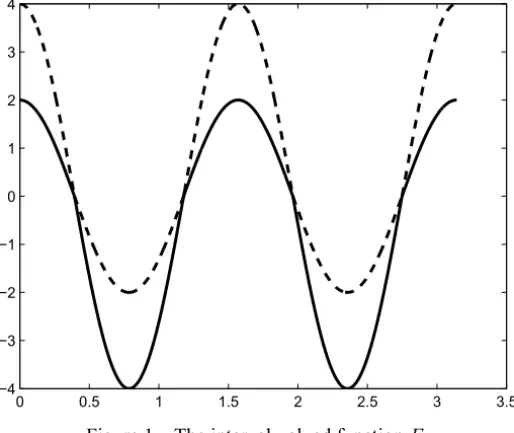
Example 4.3. We consider the interval-valued function F : [0, π] → KC defined by
F(t)= [2,4]cos(4t),
or equivalently
F(t)=
[2 cos(4t),4 cos(4t)] if 0≤t ≤π/8; [4 cos(4t),2 cos(4t)] if π/8≤t ≤3π/8; [2 cos(4t),4 cos(4t)] if 3π/8≤t ≤5π/8; [4 cos(4t),2 cos(4t)] if 5π/8≤t ≤7π/8; [2 cos(4t),4 cos(4t)] if 7π/8≤t ≤π.
Sinceg(t)=cos(4t)is a continuously differentiable function thenF is
contin-uouslyg H-differentiable and F′(t)= [−16,−8]sin(4t). So, F′
∞=16. On the other hand,Fhas seven switching points for itsg H-differentiability in
(0, π )which are{π/8, π/4,3π/8, π/2,5π/8,3π/4,7π/8}.
Figure 1 shows the endpoint functions of F, the solid line curve represent the lower function f and the dashed one represent the upper function f.
The left hand of the inequality (7) is given by
H 1
π
Z π 0
[2,4]cos(4t)dt , Fπ
8
= H 1
π[−2,2],{0}
= 2
π
while the right hand is
16 π 8
2
+ 78π2
2π
!
=16
50
π
128
0 0.5 1 1.5 2 2.5 3 3.5 −4
−3 −2 −1 0 1 2 3 4
Figure 1 – The interval-valued functionF.
So, the inequality (7) is valid forF.
Note that the inequality (7) is valid for any continuously g H-differentiable interval-valued function on[a,b]with a finite number of switching points. From the example above we can see thatFis continuouslyg H-differentiable and (7) is valid however the endpoint functions are not necessarely differentiables. For this special case, when endpoint functions are differentiables we have the following result, where we omitted thatF has a finite number of switching points.
Theorem 4.4.Let F : [a,b] →KCbe an interval-valued function such that the
endpoint functions f , f are continuously differentiables. Then, F is continuously g H differentiable and for x ∈ [a,b]
H
1
b−a
Z b
a
F(y)dy,F(x)
≤F′
∞
(x−a)2+(b−x)2
2(b−a)
. (8)
Proof. Taking in account the Ostrowski inequality (1) we have
H
1
b−a Z b
a
F(y)dy,F(x)
= H
1
b−a
Z b
a
h
f(y), f(y)
i dy,
h
f(x), f(x)
= H
1
b−a
Z b
a
f(y)dy, 1
b−a
Z b
a
f(y)dy
,
h
f(x), f(x)
i = max 1
b−a Z b
a
f(y)dy− f(x)
, 1
b−a Z b
a
f(y)dy− f(x)
≤ max f ′ ∞
(x −a)2+(b−x)2
2(b−a)
, f ′ ∞
(x−a)2+(b−x)2
2(b−a)
=
(x−a)2+(b−x)2
2(b−a)
max
f′ ∞ , f ′ ∞
= F′
∞
(x−a)2+(b−x)2
2(b−a)
.
Thus, the proof is completed.
Next we present another one generalization of the Ostrowski type inequal-ity (1).
Theorem 4.5. Let the interval-valued function F : [a,b] →Kcg H
-different-iable in(a,b)such that the endpoint functions f , f are continuously
different-iables. Letα : [a,b] → [a,b]andβ :(a,b] → [a,b],α(x)≤ x ,β(x)≥ x. Then, for all x ∈ [a,b]we have
H Z b
a
F(t)dt , (β(x)−α(x))F(x)+(b−β(x))F(b)+(α(x)−a)F(a)
≤ F′ ∞ 1 2 b −a 2 2 +
x−a+b 2
2
+
α(x)−a+x 2
2
+
β(x)−b+x 2
2
.
Proof. From Theorem 47 in [11] and properties of Hausdorff metric, we have that
H Z b
a F
(y)dy, (β(x)−α(x))F(x)+(b−β(x))F(b)+(α(x)−a)F(a)
=H Z b
a
f(y),f(y)
dy, (β(x)−α(x))
f(x),f(x)
+(b−β(x))
f(b), f(b)
+(α(x)−a)
f(a),f(a)
=max Z b a f
(y)dy−(β(x)−α(x))f(x)+(b−β(x))f(b)+(α(x)−a)f(a)
, Z b a f
(y)dy−(β(x)−α(x))f(x)+(b−β(x))f(b)+(α(x)−a)f(a)
≤max f ′ ∞ 1 2
b−a 2
2
+
x−a+b
2 2
+
α(x)−a+x
2 2
+
β(x)−b+x
2 2 , f ′ ∞ 1 2
b−a 2
2
+
x−a+b
2 2
+
α(x)−a+x
2 2
+
β(x)−b+x
2 2 =max f ′ ∞ , f ′ ∞ 1 2
b−a 2
2
+
x−a+b
2 2
+
α(x)−a+x
2 2
+
β(x)−b+x
2 2 = F′ ∞ 1 2
b−a 2
2
+
x−a+b
2 2
+
α(x)−a+x
2 2
+
β(x)−b+x
2 2
So, the inequality is established.
Remark 4.6. As a consequence of Theorem 4.5 we have the following special inequality: Let the interval-valued function F: [a,b] →Kcsatisfying the same
conditions of Theorem 4.5. Then, ifα(x) = a+x2 andβ(x) = b+x2 we have, for
all x ∈ [a,b],
H
Z b
a
F(t)dt , b−a
2
F(x)+
x
−a
b−a
F(a)+
b
−x
b−a
F(b)
≤ 1 2 F′ ∞ " b−a
2
2
+
x −a+b 2
Finally, we stablish that:
a) For this functionsαandβwe get the best bound for anyx ∈ [a,b]because the inequality in Theorem 4.5 contains a sum of squares and the minimun of this expresion occurs when each quadratic terms are zero.
b) If x = a+b2 (the midpoint of [a,b]) we obtain an even more accurate formula from Remark 4.6. In fact,
H
Z b
a
F(t)dt , b−a
2
F
a
+b
2
+ F(a)+F(b) 2
≤ 1 2
F′
∞
b
−a
2
2
REFERENCES
[1] G.A. Anastassiou,Advanced Inequalities. World Scientific, New Jersey (2011). [2] G.A. Anastassiou,Fuzzy Ostrowski type inequalities. Computational and Applied
Mathematics,22(2003), 279–292.
[3] G.A. Anastassiou, Ostrowski type inequalities. Proc. AMS,123 (1995), 3775– 3791.
[4] S.M. Assev,Quasilinear operators and their application in the theory of multival-ued mappings. Proc. Steklov Inst. Math.,2(1986), 23–52.
[5] J.P. Aubin and A. Cellina, Differential Inclusions. Springer-Verleg, New York (1984).
[6] J.P. Aubin and H. Franskowska,Introduction: Set-valued analysis in control the-ory. Set-Valued Analysis,8(2000), 1–9.
[7] J.P. Aubin and H. Franskowska,Set-Valued Analysis. Birkhäuser, Boston (1990). [8] B. Bede and S.G. Gal, Generalizations of the differentiability of fuzzy number valued functions with applications to fuzzy differential equation. Fuzzy Sets and Systems,151(2005), 581–599.
[9] Y. Chalco-Cano, H. Román-Flores and M.D. Jiménez-Gamero, Generalized derivative andπ-derivative for set-valued functions. Information Science, 181 (2011), 2177–2188.
[11] S.S. Dragomir and T.M. Rassias,Ostrowski Type Inequalities and Applications in Numerical Integration. Kluwer Academic Publishers, London (2002).
[12] M. Hukuhara,Integration des applications mesurables dont la valeur est un com-pact convexe. Funkcialaj Ekvacioj,10(1967), 205–223.
[13] S. Markov, Calculus for interval functions of a real variable. Computing, 22(1979), 325–377.
[14] R.E. Moore,Interval Analysis. Prince-Hall, Englewood Cliffs, NJ (1966). [15] R.E. Moore, Computational Functional Analysis. Ellis Horwood Limited,
Eng-land (1985).
[16] A. Ostrowski,Über die adsolutabweichung einer differentiebaren funktion von ihrem integralmittelwert. Comment. Math. Helv.,10(1938), 226–227.
[17] M.A. Rojas-Medar, M.D. Jiménez-Gamero, Y.Chalco-Cano and A.J. Viera-Brandão, Fuzzy quasilinear spaces and applications. Fuzzy Sets and Systems, 152(2005), 173–190.
[18] A. Rufián-Lizana, Y. Chalco-Cano, M.D. Jiménez-Gamero and H. Román-Flores, Calculus for interval-valued functions using generalized Hukuhara derivative and applications, Submitted.
[19] L. Stefanini and B. Bede, Generalized Hukuhara differentiability of interval-valued functions and interval differential equations. Nonlinear Analysis, 71 (2009), 1311–1328.