www.scielo.br/rbg
TERDIURNAL TIDES IN THE MLT REGION OVER CACHOEIRA PAULISTA (22.7
◦S; 45
◦W)
Aparecido Seigim Tokumoto
1, Paulo Prado Batista
2and Barclay Robert Clemesha
3Recebido em 26 janeiro, 2006 / Aceito em 13 julho, 2006 Received on January 26, 2006 / Accepted on July 13, 2006
ABSTRACT.Five years of winds measurements obtained by a SkiYmet meteor radar at Cachoeira Paulista (22.7◦S, 45.0◦W) are used to investigate the terdiurnal tide. This type of tide is frequently observed in the meteor region but the mechanisms responsible for its production are not yet completely explained. Among the possible causes are solar direct forcing and nonlinear interactions between the diurnal and semidiurnal tides. Nonlinear interaction between diurnal and semidiurnal tides can generate two secondary waves: a diurnal tide and a terdiurnal tide. The origin and seasonal distribution of the terdiurnal tide may indicate the presence of a secondary diurnal tide as a cause of variability in the primary diurnal tide. In this work we analyze the winds data in search of evidence for these mechanisms.
Keywords: atmosphere nonlinear interaction between waves, atmospheric tides.
RESUMO.Neste trabalho s˜ao usados cinco anos de medidas obtidas por um radar mete´orico, modelo SkiYmet, localizado em Cachoeira Paulista (22.7◦S, 45.0◦W), para investigar a mar´e terdiurna. Este tipo de mar´e ´e observado freq¨uentemente na regi˜ao mete´orica, por´em o mecanismo respons´avel pela sua produc¸˜ao ainda n˜ao ´e completamente explicado. Dentre as poss´ıveis causas est˜ao o forc¸ante solar direto e a interac¸˜ao n˜ao linear entre as mar´es diurna e semidiurna, que pode gerar duas ondas secund´arias: uma mar´e diurna e uma mar´e terdiurna. A origem e distribuic¸˜ao sazonal da mar´e terdiurna podem indicar a presenc¸a de uma mar´e diurna secund´aria como causa da variabilidade na mar´e diurna prim´aria. Neste trabalho n´os analisaremos os dados de vento em busca da evidˆencia destes mecanismos.
Palavras-chave: atmosfera, interac¸˜ao n˜ao linear entre ondas, mar´es atmosf´ericas.
1National Institute for Space Research, Av. dos Astronautas, 1758, Jardim da Granja – 12227-010 S˜ao Jos´e dos Campos, SP, Brazil. Phone: +55 (12) 3945-6958 – E-mail: [email protected] or [email protected]
2National Institute for Space Research, Av. dos Astronautas, 1758, Jardim da Granja – 12227-010 S˜ao Jos´e dos Campos, SP, Brazil. Phone: +55 (12) 3945-7143 – E-mail: [email protected]
INTRODUCTION
Atmospheric solar tides are global-scale waves with periods that are harmonics of a solar day. Migrating tidal components propa-gate westward with the apparent motion of the sun. These com-ponents are thermally driven by the periodic absorption of solar radiation throughout the atmosphere (Chapman & Lindzen, 1970; Forbes, 1982).
Particularly, the diurnal tide (one day period) is one of the dominant oscillations detected in the mesosphere and lower thermosphere (MLT) in the tropics. This wave is important in at-mospheric dynamics because it represents one of the mechanisms for transferring energy and momentum from the lower to the upper atmosphere (Chang & Avery, 1997). Other tidal components are the semidiurnal tide (half-day period) and the terdiurnal tide (third of a day period).
The climatology of atmospheric tides in the 70 to 110 km re-gion has been studied for many years by observations and nume-rical simulations (Avery et al., 1989; Manson et al., 1989; Vial, 1986; Forbes & Hagan, 1988, Hagan et al., 1995). Tokumoto (2002) and Batista et al. (2004) studied the climatology of the atmospheric tides and mean winds in the 80 to 100 km over Cachoeira Paulista.
The terdiurnal tides have been less studied than the diurnal and semidiurnal wind components, because, being the third har-monic in the wind decomposition, one could expect that its am-plitude would be relatively small anywhere. However, Cevolani & Bonelli (1985) found that at middle latitude, its amplitude was comparable to the diurnal tide. Cevolani (1987) and Manson & Meek (1986) found a more irregular phase variation and wave-lengths shorter in summer than in winter and amplitude higher in winter than in summer.
A numerical study by Teitelbaum et al. (1989) looked at two possible mechanisms for the excitation of the terdiurnal tide: the direct thermal generation by the third harmonic of solar daily cy-cle and dynamical generation by nonlinear interaction between the diurnal and semidiurnal tides. In this latter process, the ternal tide (zoternal wavenumber 3) is generated by the sum of diur-nal and semidiurdiur-nal (wavenumbers 1 and 2, respectively) and the difference leads to the generation of another diurnal tidal compo-nent. They found that a superposition of two tides, a propagating tide forced by solar absorption in the lower to middle atmosphere and a tide generated locally by the nonlinear wave-wave interac-tion mechanism, is consistent with the observed terdiurnal tidal structure in the summer upper mesosphere. During winter the ti-dal structure is more consistent with direct solar forcing of the terdiurnal tide.
The model of Smith & Ortland (2001) indicates that the direct solar forcing of the terdiurnal tide is the dominant mechanism at middle and high latitudes and nonlinear interactions contribute to the low latitude tide.
In this work we analyze the terdiurnal tide distribution and the nonlinear interaction between diurnal and semidiurnal tides as a possible mechanism for generation of that tidal component.
MEASUREMENTS AND DATA ANALYSIS
The 5-year data series used in this study are from a SkiYmet meteor radar at Cachoeira Paulista (22.7◦S; 45◦W). This radar
measures wind parameters from meteor trails and operates at the frequency of 35.24 MHz (Hocking et al., 2001). In this work we used data from April 1999 to March 2004.
In order to calculate wave components from wind data we used three techniques: Harmonic analysis, Lomb-Scargle periodogram and bispectral analysis.
Harmonic analysis
In this technique the data series is separated in harmonics com-ponents, where coefficients are calculated by multiple regression using least-mean-squares fitting.
This technique was used to investigate the time-height dis-tribution of terdiurnal, semidiurnal and diurnal tides. It was ap-plied by fitting the harmonics to a 96 hour window at all heights. Meridional and zonal components were separated in amplitude and phase at 48, 24, 12 and 8 hour periods, centered at heights 80, 84, 88, 92, 96 and 100 km.
The Lomb-Scargle periodogram
The periodogram is a technique to detect the power spectrum density (PSD). The classical periodogram for evenly spaced data is traditionally calculated by discrete Fourier transform (DFT). Particularly, the Lomb-Scargle periodogram is used in situati-ons where evenly spaced data cannot be obtained (Lomb, 1975; Scargle, 1982). This technique ignores the non-equal spacing of the data and involves calculating the normal Fourier power spec-trum (PSD), as if the data were equally spaced. The Lomb-Scargle technique for unevenly spaced data is known to be a powerful way to find, and test the significance of, weak periodic signals.
The PSD is given by:
PX(ω) =
1 2 P j
Xjcosω(tj−τ )
2
P
j
cos2ω(t
j −τ )
+
P
j
Xjsinω(tj −τ )
2
P
j
sin2ω(tj −τ )
(1)
time,ωis a component of frequency, andτ is defined by
tan(2ωτ )=
P
jsin 2ωtj
P
jcos 2ωtj
(2)
The inclusion of theτ terms makes the periodogram invariant to a shift of the origin of time.
The Lomb-Scargle periodogram is equivalent to least-squares fitting of sine curves to the data and the power spectrum follows an exponential probability distribution. This exponential distribution provides a convenient estimate of the probability that a given peak is a true signal, or whether it is the result of randomly distributed noise.
In this work we calculated the power spectrum density (PSD) using a 15-day data window, and height intervals of 10 km cente-red at 85 and 95 km. This analysis makes it possible to investigate the periodic elements present in the wind. The Lomb-Scargle pe-riodogram indicates the components present in the spectrum, but not its origin.
In order to investigate the wave origin we use bispectral analysis.
Bispectral analysis
The bispectrum is, by definition, the two-dimensional Fourier transform of the third order cumulant for a real, stationary, ran-dom process,x(t). The theoretical basis of bispectrum has been reviewed by various authors (Hinich & Clay, 1968; Mendel, 1991). The computational procedure used in this work has been descri-bed by Kim & Powers (1979):
1) Form M sets of data records of length N.
2) Subtract the mean value from each record.
3) Apply an appropriate data window to each record to reduce leakage (in this work a Hanning window has been used).
4) Compute the Fourier amplitudes, using the FFT technique
5) Estimate the bispectrum by
ˆ
B(ω1, ω2) =
1
M
M
X
i=1
Xi(ω1)Xi(ω2)Xi∗(ω1+ω2) (3)
whereX(ω)is the Fourier transform ofx(t),X∗denotes the complex conjugate.
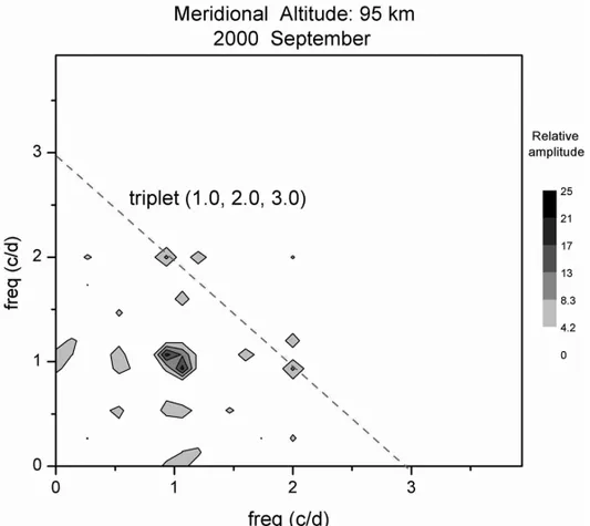
Bispectral analysis examines the relationships between the oscillations at two basic frequencies,ω1andω2, and another fre-quencyω3 =ω1+ω2. This set of three frequencies is known
as a triplet(ω1, ω2, ω3). A non-zero bispectrum value at bi-frequency(ω1, ω2)indicates that there is at least frequency cou-pling within the triplet above studied and a quadratic non-linearity is present. Frequenciesω1andω2are plotted directly in graphic, and are represented by points (with same value) at horizontal and vertical axis. The points at both axis generated by intersection of a diagonal that crosses the bispectrum values plotted in graphic correspond to the third term of triplet, i.e., frequencyω3.
To evaluate the bispectrum, in this work we used M = 5, N = 360 points (15 days) with an overlap of 96 points (4 days) between data sets.
RESULTS
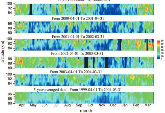
We present, in Figures 1 to 3 time-height contours for the am-plitudes of the meridional components of the terdiurnal, diurnal and semidiurnal tides respectively. Figure 4 to 6 show the same as Figures 1 to 3, but for the zonal components. In these figures, the annual distribution of the terdiurnal and diurnal tide are shown from April 1999 to March 2004. The last panel shows a five-year average of the data.
Meridional terdiurnal tidal amplitudes have a dominant se-miannual variation. Tidal amplitudes maximize above 92 km, in March and April, and in August through October (equinoctial months); in other months, the amplitudes are weak. This seasonal distribution above 92 km coincides with the semiannual diurnal and semidiurnal tidal distribution with maxima mainly in equinoc-tial months too.
The time variation for the tidal zonal components are shown in Figures 4 to 6.
Zonal terdiurnal tidal amplitudes (Fig. 4) are weaker than the meridional component with maxima above 92 km. The terdiur-nal tide is more spread out over other months than the diurterdiur-nal (Fig. 5) or semidiurnal (Fig. 6) tides, but shows a semiannual dis-tribution, with maxima at higher altitudes in equinoctial months.
We calculated periodograms and bispectra of unfiltered wind series in several segments, which are representatives of solsticial and equinoctial months in order to analyze the spectral behavior of the terdiurnal tide. The following figures show some examples for meridional components.
Figure 1– Amplitude of the terdiurnal component of the meridional wind, from April 1999 to March 2004: panels 1 to 5 (top to bottom). Five-year average: panel 6. Color scale amplitudes are in m/s.
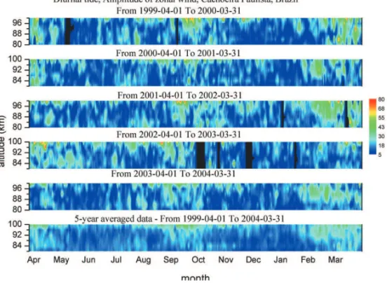
Figure 2– As Figure 1 but for the diurnal tide.
Figure 8 shows bispectra of unfiltered winds in September for meridional winds. The peaks at (1.0, 2.0) could indicate a nonlinear interaction between the diurnal and semidiurnal tide generating a terdiurnal tide (3.0).
Table 1 shows for two altitudes (85 and 95 km) when a peak in the (1.0, 2.0) appears for the meridional components for all months between 1999 and 2004.
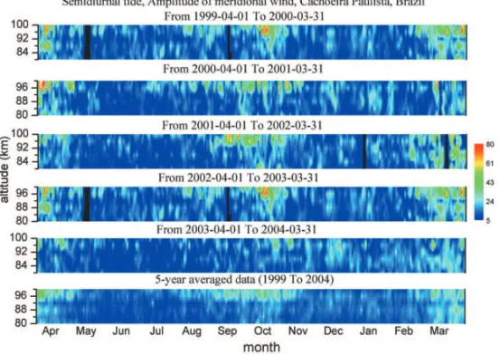
Figure 3– As Figure 1 but for the semidiurnal tide.
Figure 4– Amplitude of the terdiurnal component of the zonal wind, from April 1999 to March 2004: panels 1 to 5 (top to bottom). Five-year average: panel 6. Color scale amplitudes are in m/s.
Another possible analysis used to verify nonlinear interaction is the vertical wavelength relationship between diurnal, semidiur-nal and terdiursemidiur-nal components. The vertical wavelength is calcu-lated using vertical distribution of phases. Theoretically, in nonli-near interaction of waves, the inverse of secondary wavelength is equal to the sum or difference of the inverse of the primary wavelengths.
In this work the vertical wavelengths for the 8 h, 12 h and 24 h wind components were calculated by a linear fitting of the phases in windows of 15 days in altitudes below and above 90 km. The results are displayed in Table 2.
Table 1– Seasonal distribution of bispectra at 85 km and 95 km heights between April 1999 and March 2004. The “X” shows months in which there occurred nonlinear interactions.
85 km 95 km
Month 99/00 00/01 01/02 02/03 03/04 Month 99/00 00/01 01/02 02/03 03/04
Apr X X X X X Apr X X X
May X X X May X X X
Jun X X X Jun X X X X
Jul X X X Jul X X
Aug X X Aug X X X
Sep X X X X X Sep X X X X X
Oct X X X X X Oct X X X X X
Nov X Nov X X X X
Dec X X X X X Dec X X X X X
Jan X X X Jan X X
Feb X X X X Feb X X
Mar X X X X X Mar X X X
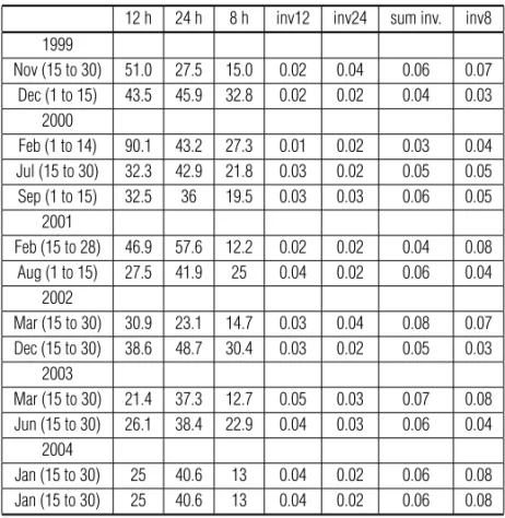
Table 2– Comparison between the inverse of 8 h meridional wavelength and the sum of the inverses of 12 h and 24 h meridional wavelengths at altitudes above 90 km. This compa-rison has been made by month and year between April 1999 and March 2004.
12 h 24 h 8 h inv12 inv24 sum inv. inv8 1999
Nov (15 to 30) 51.0 27.5 15.0 0.02 0.04 0.06 0.07 Dec (1 to 15) 43.5 45.9 32.8 0.02 0.02 0.04 0.03
2000
Feb (1 to 14) 90.1 43.2 27.3 0.01 0.02 0.03 0.04 Jul (15 to 30) 32.3 42.9 21.8 0.03 0.02 0.05 0.05 Sep (1 to 15) 32.5 36 19.5 0.03 0.03 0.06 0.05
2001
Feb (15 to 28) 46.9 57.6 12.2 0.02 0.02 0.04 0.08 Aug (1 to 15) 27.5 41.9 25 0.04 0.02 0.06 0.04
2002
Mar (15 to 30) 30.9 23.1 14.7 0.03 0.04 0.08 0.07 Dec (15 to 30) 38.6 48.7 30.4 0.03 0.02 0.05 0.03
2003
Mar (15 to 30) 21.4 37.3 12.7 0.05 0.03 0.07 0.08 Jun (15 to 30) 26.1 38.4 22.9 0.04 0.03 0.06 0.04
2004
Figure 5– As Figure 4 but for the diurnal tide.
Figure 6– As Figure 4 but for the semidiurnal tide.
24 h and 8 h components at altitudes above 90 km, columns 5 and 6 represent the inverse of 12 h and 24 h wavelengths, column 7 represents the sum of values represented in columns 5 and 6 and column 8 represents the inverse of the 8 h wavelength. Note that values in the two last columns are similar. These rela-tionships can indicate evidence of nonlinear interaction between wind components at least in these intervals.
Figure 7– Periodogram of unfiltered meridional wind for September 2000 at 95 km. 90% line is the confidence level.
Figure 8– Bispectrum of unfiltered meridional wind for September 2000 at 95 km.
CONCLUSIONS
The analysis of MLT region winds over Cachoeira Paulista reveals that meridional and zonal terdiurnal tides have semiannual fea-tures with peaks at higher altitudes at the equinoxes. This
compo-nents, and during winter almost no nonlinear interaction is pre-sent, and the terdiurnal component in this interval is probably due to direct solar excitation. These characteristics suggest that the terdiurnal tide is not an important component in MLT dynamics at our latitude. However, the seasonal and altitudinal distributions of the tides show a correlation between the diurnal and terdiur-nal components, suggesting nonlinear interaction as an important source for the terdiurnal oscillation.
ACKNOWLEDGMENTS
This work was supported by the Fundac¸˜ao de Amparo `a Pesquisa do Estado de S˜ao Paulo (FAPESP) and the Conselho Nacional de Desenvolvimento Cient´ıfico e Tecnol´ogico (CNPq).
REFERENCES
AVERY SK, VINCENT RA, PHILLIPS A, MANSON AH & FRASER GJ. 1989. High latitude tidal behavior in the mesosphere and lower thermosphere. Journal of Atmospheric and Terrestrial Physics, 51: 595–608.
BATISTA PP, CLEMESHA BR, TOKUMOTO AS & LIMA LM. 2004. Struc-ture of the mean winds and tides in the meteor region over Cachoeira Paulista, Brazil (22.7◦S, 450◦W) and its comparison with models. J. Atmospheric and Terrestrial. Physics, 66: 623–636.
CEVOLANI G & BONELLI P. 1985. Tidal activity in the middle atmosphere. Nuovo Cimento Soc. Ital. de Fisica, 8: 461–674.
CEVOLANI G. 1987. Tidal activity in the meteor zone over Budrio, Italy. Handbook MAP, 13: 166–186.
CHANG JL & AVERY SK. 1997. Observations of the diurnal tide in the mesosphere and lower thermosphere over Christmas Island. J. Geophy-sical Research, 102(D2): 1895–1907.
CHAPMAN S & LINDZEN RS. 1970. Atmospheric tides. Dordrecht: D. Reidel Publishing Company. 200 pp.
FORBES JM. 1982. Atmospheric tides. 1. Model description and results for the solar diurnal components. Journal of Geophysical Research, 87: 5222–5240.
FORBES JM & HAGAN ME. 1988. Diurnal propagating tide in the pre-sence of mean winds and dissipation: A numerical investigation. Plane-tary Space Science, 36: 579–590.
HAGAN ME, FORBES JM & VIAL F. 1995. On modeling migrating solar tides. Geophysical Research Letters, 22: 893–896.
HINICH MJ & CLAY CS. 1968. The application of the discrete Fourier transform in the estimation of power spectra, coherence and bispectra of geophysical data. Reviews of Geophysics, 6: 347–366.
HOCKING WK, FULLER B & VANDEPEER B. 2001. Real-time determi-nation of meteor-related parameters utilizing modem digital technology. Journal of Atmospheric and Solar-Terrestrial Physics, 63: 155–169.
KIM YC & POWERS EJ. 1979. Digital bispectral analysis and its ap-plications to nonlinear wave interactions. IEEE Transactions on Plasma Science, 7: 120–131.
LOMB NR. 1975. Least-squares frequency analysis of unequally spaced data: Astrophysics and Space Science, 39: 447–462.
MANSON AH & MEEK CE. 1986. Dynamics of the middle atmosphere at Saskatoon (52◦N, 107◦W): a spectral study during 1981, 1982. Journal of Atmospheric and Terrestrial Physics, 48: 1039–1055.
MANSON AH, MEEK CE, TEITELBAUM H, VIAL F, SCHMINDER R, H ¨URSCHNER R, SMITH MJ, FRASER GJ & CLARK RR. 1989. Cli-matologies of semi-diurnal and diurnal tides in the middle atmosphere (70-110 km) at middle latitudes (40-55◦). Journal of Atmospheric and Terrestrial Physics, 51(7/8): 579–593.
MENDEL JM. 1991. Tutorial on higher-order statistics (spectra) in signal processing and system theory: theoretical results and some applications. Proceedings of the IEEE, 79: 278–305.
SMITH AK & ORTLAND DA. 2001. Modeling and analysis of the structure and generation of the terdiurnal tide. Journal of Atmospheric Sciences, 58: 3116–3134.
SCARGLE JD. 1982. Studies in astronomical time series analysis. II. Statistical aspects of spectral analysis of unevenly spaced data. The astrophysical journal, 263: 835–853.
TEITELBAUM H, VIAL F, MANSON AH, GIRALDEZ R & MASSEBEUF M. 1989. Non-linear interaction between the diurnal and semidiurnal tides: terdiurnal and diurnal secondary waves. Journal of Atmospheric and Terrestrial Physics, 51: 627–634.
TOKUMOTO AS. 2002. Ventos na regi˜ao de 80-100 km de altura sobre Cachoeira Paulista (22.7◦S, 45◦W), medidos por radar mete´orico. M.Sc. Thesis, National Institute for Space Research. 132 pp.
NOTES ABOUT THE AUTHORS
Aparecido Seigim Tokumotograduated in Physics (1987) at the University of Mogi das Cruzes (UMC), Brazil and in Electrical Engineering (1993) at the University of the Para´ıba Valley (UNIVAP), Brazil. He did his M.Sc (2002) and Ph.D (2007) in Space Geophysics at the National Institute for Space Research (INPE). He is a Mathematics and Physics teacher at high school level. His areas of interest are upper atmospheric dynamics and atmospheric waves studied by meteor radar.
Paulo Prado Batistagraduated in Physics (1972) at the Federal University of Goi´as (UFG). He has been working at INPE (National Institute for Space Research) since 1973. He obtained his M.Sc (1977) and Ph.D (1983) in Space Sciences at INPE, where today he is a senior researcher. His present interests include middle atmosphere dynamics, interactions between atmospheric waves and airglow and upper atmosphere studies using lidar.