www.scielo.br/rbg
STATISTICAL STUDY OF INCOHERENT INTEGRATION APPLIED TO SIMULATED POWER SPECTRA
OF RADAR SIGNALS BACKSCATTERED FROM EQUATORIAL ELECTROJET IRREGULARITIES
Henrique Carlotto Aveiro
1, Clezio Marcos Denardini
2, Mangalathayil Ali Abdu
3and Nelson Jorge Schuch
4Recebido em 23 janeiro, 2006 / Aceito em 8 marc¸o, 2007 Received on January 23, 2006 / Accepted on March 8, 2007
ABSTRACT.Spectral analysis of radar echoes through spectral moment estimation allows to identify the characteristics of plasma irregularities from equatorial electrojet. The curve fitting using the maximum likelihood estimator (MLE) was chosen as the technique to obtain the plasma irregularity information. The implication of applying distinct number of incoherent integration to simulated Type 1 plasma irregularity radar spectra is investigated. The response of the fitting is evaluated using the covariance matrix of the MLE. A statistical study of incoherent integration applied to equatorial electrojet plasma irregularity spectra is presented in order to determine its effects over the estimation of Doppler velocities. The optimal values of incoherent integrations in relation to the goodness of the fitting are obtained in order to better determine the Type 1 plasma irregularity characteristics.
Keywords: ionosphere, aeronomy, radar, digital signal processing, curve fitting.
RESUMO.A an´alise espectral de ecos de radar atrav´es da estimac¸˜ao dos momentos espectrais permite a identificac¸˜ao das caracter´ısticas das irregularidades de plasma das irregularidades do eletrojato equatorial. Dentre as t´ecnicas usadas para obtenc¸˜ao das informac¸˜oes de irregularidades de plasma, ´e utilizado o ajuste de curvas pela estimac¸˜ao de m´axima verossimilhanc¸a. Este trabalho analisa a aplicac¸˜ao de valores distintos de integrac¸˜ao incoerente a espectros simulados de radar de irregularidades de plasma do Tipo 1. A resposta do ajuste ´e avaliada utilizando a matriz de covariˆancias do estimador de m´axima verossimilhanc¸a. Um estudo estat´ıstico da integrac¸˜ao incoerente aplicado a espectros de irregularidades do EEJ ´e apresentado de modo a determinar seus efeitos sobre a estimac¸˜ao das velocidades Doppler. Os valores ´otimos de integrac¸˜oes incoerentes em relac¸˜ao `a qualidade do ajuste s˜ao obtidos de forma a melhor determinar as caracter´ısticas de irregularidades de plasma do Tipo 1 do EEJ.
Palavras-chave: ionosfera, aeronomia, radar, processamento de sinais digitais, ajuste de curvas.
1Southern Regional Space Research Center, National Institute for Space Research, Av. Roraima, s/n, Bairro Camobi, P.O. Box 5021 – 97110-970 Santa Maria, RS, Brazil. Phone: +55 (55) 3220-8021; Fax: +55 (55) 3220-8007 – E-mail: [email protected]
2National Institute for Space Research, Av. dos Astronautas, 1.758, Jardim da Granja, P.O. Box 515 – 12227-010 S˜ao Jos´e dos Campos, SP, Brazil. Phone: +55 (12) 3945-7156; Fax: +55 (12) 3945-6990 – E-mail: [email protected]
3National Institute for Space Research, Av. dos Astronautas, 1.758, Jardim da Granja, P.O. Box 515 – 12227-010 S˜ao Jos´e dos Campos, SP, Brazil. Phone: +55 (12) 3945-7149; Fax: +55 (12) 3945-6990 – E-mail: [email protected]
INTRODUCTION
The equatorial electrojet (EEJ) is an electric current that flows in the height region from about 90 to 120 km (at ionospheric E-region), covering a latitudinal range of±3◦around the dip
equa-tor (Forbes, 1981). It is driven by the E-region dynamo electric field (Fejer & Kelley, 1980) and represents an important aspect of the phenomenology of the equatorial ionosphere-thermosphere system. Sounding observations of the equatorial ionospheric E-region using VHF radars have shown backscattered echoes from electron density irregularities in the EEJ in several sectors, such as the Peruvian sector (Cohen & Bowles, 1967; Balsley, 1969; Cohen, 1973; Fejer et al., 1975; Farley, 1985), the Indian sec-tor (Prakash et al., 1971; Reddy & Devasia, 1981; Somayajulu et al., 1991), and the Brazilian sector (Abdu et al., 2002; Abdu et al., 2003; de Paula & Hysell, 2004; Denardini et al., 2004; Denardini et al., 2005). These echoes contain Doppler shifted frequency components due to the drift of the irregularities. The echoes present distinct spectral signatures called Type 1 and type 2 spectra. The type 1 spectrum is produced by irregularities gene-rated by the two-stream plasma instability process (Farley, 1963; Buneman, 1963) and the type 2 is originated from the gradient drift instability mechanism (Rogister & D’Angelo, 1970). Several experiments have been conducted to investigate the EEJ irregula-rities in order to characterize its spectra and explain the pheno-menology (Reddy, 1981; Fejer & Kelley, 1980; Forbes, 1981, and references therein).
In the Brazilian sector a 50 MHz coherent backscatter ra-dar, also known by the acronym RESCO (in Portuguese, Radar de ESpalhamento COerente), has been operated since 1998 at S˜ao Lu´ıs, State of Maranh˜ao (2.33◦S, 44.2◦W, DIP: –0.5), on
the dip equator. Observations of EEJ 3-m plasma irregulari-ties are routinely carried out with the main purpose of studying the EEJ dynamics through spectral analysis of the backscatte-red echoes from plasma instabilities. For such studies, a pre-cise determination of the spectral moments of the irregulari-ties is a crucial requirement. Several techniques for estima-ting Doppler shifts based on radar power spectra have been developed and reviewed (May & Strauch, 1989; May et al., 1989; Woodman, 1985). In the present work we have estima-ted the irregularity Doppler shifts by fitting two Gaussians to each power spectrum using the Least Squares Fitting Method (Levenberg, 1944; Marquardt, 1963; Press et al., 1992). In this case, the quality of the fitting will depends on the variance of the noise present in the spectrum. And a well-known tool to reduce variance of the noise is the incoherent integrations, a technique
that does not change the mean spectral densities of both signal and noise. Increasing the number of integrated spectra means to reduce the variance and to define better the power spectra. In this way we have used the incoherent integration technique applied to simulated power spectra of radar signals like it was backs-cattered from equatorial electrojet irregularities type 1 to quan-tify the advantages and disadvantages of applying such technique. In the following section we present the typical radar data proces-sing, a brief description of the spectra simulations, and the results of this statistical study, which are discussed in terms of good-ness of the estimates and the variance of the estimate Doppler frequency type 1.
RADAR DATA PROCESSING AND THE INCOHERENT INTEGRATION
The current RESCO data processing consist in fitting the sum of two Gaussians (each one representing one type of irregularity) both having a white noise level to each Doppler power spectra, which usually has an aliasing frequency of 250-500 Hz after being obtained from the Fast Fourier Transform (FFT) of the received echoes. The frequency resolution will depend upon the aliasing frequency and the number of sequential pulses. For the present study we have chosen the frequency resolution to be about 1 Hz. This processing is made based on the assumption that each spec-trum is described by a S distribution in function of the frequency, given by:
S(f) = P1 σ1
√
2π exp "
−(f − fd1) 2
2σ12 #
+ P2
σ2 √
2π exp "
−(f − fd2) 2
2σ22 #
+PN, (1)
where PN, Pi,σi and fdi are the noise level, spectral power,
spectral width and Doppler frequency, respectively. Thei index indicates the type of the described irregularity: type 1 (i = 1) or type 2 (i= 2). The Maximum Likelihood Estimate (MLE) has been used for nonlinear fitting of the 7 parameters of each spectrum,a
={fd1, fd2, σ1, σ2,P1,P2,PN}. The fitting method is based
on finding the parametersathat maximize the probability func-tionP(y1. . .yn|a)of obtaining the data sety= {y1. . .yn}. In other words, it is a problem of finding the parametersathat minimize the square sum of residual errors between the observa-tional data setyand the corresponding GaussiansS(f)that des-cribes the data set, considering the uncertaintyσirelated to each
mathema-tically the above statement.
χ2≡ N X
i=1
yi−S fi,P1, fd1, σ1,P2, fd2, σ2,PN2 σi
(2)
Here, N is the number of frequencies in the power spectrum,
yi is the observed spectral amplitude for a given frequency and all the other parameters have been introduced before. Despite curve fitting algorithm being largely used, it usually does not pre-sent satisfactory results when the variance is too high. One of the solutions to reduce high variances is to integrate incoheren-tly several consecutive spectra. The method consists in averaging the power spectral density at a given frequency from several con-secutive spectra, for all frequencies in the spectrum. Since the white noise is a random component, the resulting spectrum will have lower variance. Figure 1 presents an illustration of the re-sulting spectrum (on the right side) from incoherent integration of hundred consecutive spectra (on the left side), where a noisy bunch of spectra (represented by the first one) became a smo-othed one. The incoherent integration reduces the variance of the noise(σN2)and better defines the power spectra, but it does not change the mean values of signal(P)and noise spectral(PN) densities (Fukao, 1989). In a spectrum without incoherent inte-gration,σNis equal toPN. But, the unitary ratioσN/PNdecays
with the inverse of the square root of the number of incoherent integrations(N I C H), i.e., σN becomes equal to the relation PN/(N I C H)1/2.
SIMULATION AND PROCESSING OF POWER SPECTRA
This work focuses on the study of the effects of incoherent integration on the type 1 power spectra of backscattered signals from 3-m EEJ plasma irregularities. This class of spectrum nor-mally presents a sharp peak centered at around 120 Hz, which corresponds to a Doppler shift of about 360 m/s (ion-acoustic speed) for radars operating at 50 MHz. So, the Gaussian co-variance model of Zrnic (1979) was used to simulate groups of one thousand Gaussian like power spectra. Each power spectrum being constituted of 256 data points with typical characteristics of type 1 irregularities (fd = 120 Hz,σ = 20 Hz). White noise was added at 6 dB signal-to-noise ratio(S N R)in time domain in order to assure a more realistic variance in the power spec-tra. Theses groups were arranged and those spectra were inte-grated incoherently in such a way that we always have one thou-sand power spectra per group and each group represents one dif-ferent value ofN I C H: 1, 2, 4, 6, 8, 10, 20, 40, 60, 80 and 100. In summary, Eq. (2) was simplified to a case of a single Gaussian
described by aSdistribution in function of the frequency, as given per equation (3).
S(f) = P σ√2π exp
"
−(f − fd) 2
2σ2
#
+PN (3)
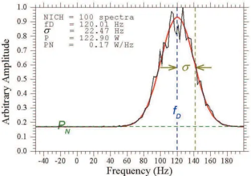
The quantities in this equation are the same as describe for equa-tion 1 and refer to a type 1 Gaussian. Figure 2 presents an example of a spectrum simulated as above. The superimposed color lines (accompanied by their respective symbols) indicate the quantities mentioned in the power spectrum. The green line represents the power density of the noise(PN). The vertical blue line shows the center of frequency distribution(fd). The difference between the brown and blue vertical lines determines the standard deviation of the fitted curve. And the area between the red and the green line defines the signal power(P).
The data sets of power spectra simulated as described here were processed as ordinary spectra obtained in the RESCO data processing. We have used MLE to minimize the square sum of residual error in a way to fit a Gaussian (Eq. 3). The same algo-rithm has fitted each spectrum of the eleven data set groups to a single Gaussian. And the basic analysis consisted in to compare directly the fdfitted to the spectra using Gaussians to thea priori fdvalue used to generate the type 1 spectra during the spectra simulation. Moreover, the goodness of the fitting was analyzed in function of the number of incoherent integrations and the variance of the estimated parameters as well.
RESULTS AND DISCUSSIONS
ORIGINAL SPECTRA MEAN SPECTRUM
Figure 1– Illustration of incoherent integration applied to hundred consecutive spectra (left) and the resultant spectrum (right).
Figure 2– Power spectrum resulting from the incoherent integration of one hundred simulated power spectra (black line) superimposed by a Gaussian curve (red line) fitted to the spectrum using Least Square Error Method. The green line represents the noise power density(PN), the vertical blue line shows the center of frequency distribution(fd),
the difference between the vertical brown and blue lines determines the standard deviation of the Gaussian curve fitted to the spectrum(σ )and the area between the red and the green line defines the power of the signal(P).
observational time increases directly proportional to the number of spectra used in the integration.
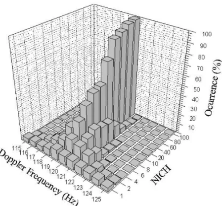
The percentage of answers close to thea priori fd value (120±0.5 Hz) in function ofN I C H is presented in Table 1. The averaged variances of the spectral moments (fd, Pandσ) estimated from the method and the noise power(PN)obtained by the covariance matrix of the chi-squared distribution (from Eq. 2) are showed in the same table. These results show that the efficiency of the method increased from 9.20% to 99.50%, with a statistical error of 0.42% (±0.5 Hz), when it goes from no incoherent integration (NICH = 1) to the incoherent integration of
100 consecutive spectra.
The analysis of the variances of the estimate moments gi-ves us an indication of the accuracy of each parameter for the given SNR (6 dB in the present case). Table 1 shows that the higher the N I C H the lower the variances. A clear example is the high variance ofσwhen no incoherent integration is applied. This indicates the curve fitting hardly ever have good estimates for this parameter. Our results had shown that increasing N I C H
Figure 3– Percentage of occurrences of Doppler Frequencies estimated by MLE using spectra with no incoherent integration and integration of 2, 4, 6, 8, 10, 20, 40, 60, 80 and 100 spectra. Each Doppler frequency is centered in the integer frequency defined in the axis with±0.5 Hz of resolution.
Table 1– Percentage of answers close to thea priori fdvalue (120±0.5 Hz) in function ofN I C H
and the variances of spectral power, Doppler frequency, spectral width and noise.
Good Variance Variance Variance Variance
NICH estimates of estimate of estimate of estimate of estimate
(%) fd(Hz2) σ(Hz2) PN(10-9W2/Hz2) P(10-6W2)
1 9.20 4.6455 12.1841 18.527 4.8421
2 20.70 2.0206 0.9342 22.205 4.2802
4 33.20 0.9588 0.4389 15.841 2.8436
6 44.30 0.6303 0.2877 11.812 2.0767
8 52.00 0.4689 0.2142 9.342 1.6248
10 54.40 0.3738 0.1707 7.707 1.3311
20 74.20 0.1857 0.0849 4.090 0.7025
40 90.80 0.0927 0.0424 2.112 0.3596
60 94.20 0.0617 0.0282 1.422 0.2414
80 98.30 0.0462 0.0211 1.072 0.1824
100 99.50 0.0370 0.0169 0.859 0.1460
The last two parameters of Table 1 indicate good results af-ter incoherent integration. The variance of estimatePN reduces itself more than 20 times increasingN I C Hfrom 1 to 100 spec-tra. It means that the white noise level is better defined, separating that one from the information of the Gaussian curve. Table 1 still shows that the variance of estimatePis more than 30 times better determined after 100 spectra incoherent integrations. It indicates
a better definition of the intensity of the turbulence, since they are proportional to each other.
The graph of Figure 4 shows the mathematical relationship between the number of integrated spectra and the number of oc-currences close to thea priori fdvalue (120±0.5 Hz). The dots give the Percentage of Right Estimated Answers(P R E A)for
named saturation marks the maximum possible value of percen-tage, i.e, 100% of occurrences. This figure clearly shows a loga-rithmic dependence of the percentage of right answers from the number of incoherent integrations. In order to quantify this rela-tion, we have performed a linear fitting like logarithmic growth on this data, represented by the curve superimposed to the Figure 4. The following equation has been used for this fitting:
P R E A = α∙ln(N I C H)+β,
1≤ N I C H≤100, (4)
where P R E A is the Percentage of Right Estimated Answers, αcould be considered as a growing rate of P R E Aandβ is the P R E A observed when no incoherent integrations is ap-plied to the data set. The fitting resulted anα= 21.01±0.66 and aβ = 7.46±1.93, with a quadratic correlation factor as R2 = 0.9912. The points with lower N I C H are better fitted
than the higher ones because the points are closer to each other for lower N I C H (2, 4, 6, 8 and 10) that for higher N I C H
(20, 40, 60, 80 and 100). Despite the logarithmic growing (curve of Fig. 4) did not fit perfectly to the data (dots) at high N I C H
values, we have obtained a quadratic correlation factor higher then 99%. Moreover, we expect a better fitting of the logarith-mic growing curve forN I C Hhigher than 100. The step that the good estimates increases as we increase the number of incohe-rent integrations is also an interesting result. For instance, when the N I C H is increased from 60 to 100 the P R E A differs in less than 6%, but the observational time increases by almost 66%. This indicates there should be some optimal point above of which increases in theN I C H do not substantially improve theP R E Awithout compromise the observational time. Finally, this results show that in case of using incoherent integration one must choose the lowest number of incoherent integration as pos-sible, i.e., before the asymptotic region in the logarithmic law (Eq. 4). We should also remember that Eq. (4) is a result of the analysis from simulated data and we may obtain higher or lower values of standard deviation of the noise(σN)in a case of real
spectra of radar. So, in spite of Eq. (4) does not give a descrip-tion for real cases, it is expected that the logarithmic characteris-tic betweenP R E AandN I C Hremains valid, being helpful to a qualitative analysis.
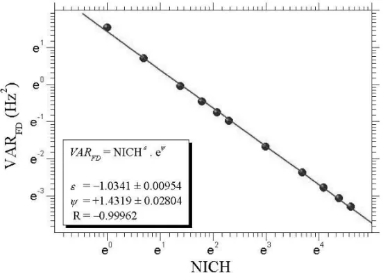
Other point we would like to address in this paper is the de-pendence of the averaged variance of fd(V A RF D)from the number of integrated spectra(N I C H). Figure 5 presents the mathematical relationship between the averaged variance (dots) and the number of incoherent integration. The graph clearly shows a linear dependence between the natural logarithmic of variance
of fd and the natural logarithmic of the incoherent integrations. In order to quantify the dependence, we have performed a linear fitting to these data in ln-ln domain, represented by the curve su-perimposed to the graph on Figure 5. The following equation has been used to fit the data:
V A Rf d = N I C Hε∙eψ,
1≤N I C H ≤100, (5)
whereV A Rf d is the fitted variance of estimate fd, εis the
negative power coefficient that tell us how much theV A Rf d
reduces as we increase theN I C H, and the exponential ofψ is theV A Rf d observed when no incoherent integration is
ap-plied. The power coefficientεresulted –1.0341 (±0.00954). Theψfactor resulted 1.43189 (±0.02804). And the correlation factor R resulted –0.99962. Observe that the negative power co-efficient is very close to the unit. This indicates that increases in the number of spectra incoherently integrated will almost propor-tionally decrease the variance of the estimate Doppler frequency. Also, when no incoherent integration is applied the power coef-ficient effect will be negligible. And the variance will be given by the exponential ofψ factor. Therefore, Eq. (5) in this sim-ple form seems to give a comprehensive idea of how the variance will behave as we apply incoherent integrations to our data set. Higher values ofN I C Hwill proportionally reduce the variance of the estimate Doppler frequency. On the other hand, it will also proportionally increase the observational time. Consequently, the compromise of the observational time seems to be linear rela-ted to the increase of the number of incoherent integration and to the decrease of the variance. Moreover, theψ factor seems to be related to SNR of the data set. Reductions in to the SNR will probably reduceψfactor. Hence, this factor should be related to noise level on the radar system.
Finally, applying incoherent integrations to the observational radar spectra of type 1 equatorial electrojet irregularities means a compromise among the percentage of right estimated answers when using MLE techniques for estimating the Doppler frequency, the variance of the estimate Doppler frequency and the observa-tional time. For the present study we have observed that small numbers of incoherent integrations decreases substantially the variance of the estimate Doppler frequency as well as increases the percentage of right estimated answers, without much com-promise to the observational time. Larger number of incoherent integrations will fall into the asymptotic region of the P R E A
Figure 4– Percentage of right estimated answers(P R E A)in function of the number spectra used in the in-coherent integrations(N I C H). The analyzed incoherent integrations are the dots and the logarithmical fitting is the curve. The dashed line shows the saturation ofP R E A, i.e, 100% of occurrences.
Figure 5– Averaged variance of fdassociated with the fitting method(V A RF D)in function of the number
spectra used in the incoherent integrations(N I C H). The analyzed incoherent integrations are the dots and the logarithmical fitting is the curve.
CONCLUSIONS
The technique of incoherent integration has shown to be a va-luable tool, which is able to improve significantly the estimates of the test parameter (the center of the frequency distribution of the power spectra from the radar echoes of the EEJ irregularities).
in this paper the linear dependence of the natural logarithmic of variance of the estimate fdand the natural logarithmic of the in-coherent integration. The power coefficientεfrom linear fitting indicated that increases in the number of spectra incoherently in-tegrated will almost proportionally decrease the variance of the estimate Doppler frequency. In addition, we have found an expo-nential factorψ, which we believe to be related to SNR of the data set. Reducing the SNR will probably reduce this factor. Finally, we have seen that applying incoherent integrations to the obser-vational radar spectra of type 1 equatorial electrojet irregularities means to increase the percentage of right estimated answers when using MLE techniques for estimating the Doppler frequency, but we have to balance the variance of the estimate Doppler frequency and the observational time.
ACKNOWLEDGMENTS
The first author wishes to thank CNPq/MCT for financial support to his undergraduate program through the project 107616/2003-3. The second author wishes to thank FAPESP (2005/01113-7) for the financial support to attend the 9th CISBGf in which congress this work has been presented.
REFERENCES
ABDU MA, DENARDINI CM, SOBRAL JHA, BATISTA IS, MURALI-KRISHNA P & DE PAULA ER. 2002. Equatorial electrojet irregularities investigations using a 50 MHz back-scatter radar and a Digisonde at S˜ao Lu´ıs. Some initial results. Journal of Atmospheric and Solar-Terrestrial Physics, 64(12-14): 1425–1434.
ABDU MA, DENARDINI CM, SOBRAL JHA, BATISTA IS, MURALI-KRISHNA P, IYER KN, VELIZ O & DE PAULA ER. 2003. Equatorial electro-jet 3 m irregularity dynamics during magnetic disturbances over Brazil: results from the new VHF radar at S˜ao Lu´ıs. Journal of Atmospheric and Solar-Terrestrial Physics, 65(14-15): 1293–1308.
BALSLEY BB. 1969. Some Characteristics of Non-2-Stream Irregulari-ties in Equatorial Electrojet. Journal of Geophysical Research, 74: 2333– 2347.
BUNEMAN O. 1963. Excitation of field aligned sound waves by electron streams. Physical Review Letters, 10(7): 285–287.
COHEN R & BOWLES KL. 1967. Secondary Irregularities in Equatorial Electrojet. Journal of Geophysical Research, 72: 885–894.
COHEN R. 1973. Phase Velocities of Irregularities in Equatorial Electro-jet. Journal of Geophysical Research, 78: 2222–2231.
DE PAULA ER & HYSELL DL. 2004. The S˜ao Lu´ıs 30 MHz coherent scatter ionospheric radar. System description and initial results. Radio Science, 39(1): 1–11.
DENARDINI CM, ABDU MA & SOBRAL JHA. 2004. VHF radar stu-dies of the equatorial electrojet 3-m irregularities over S˜ao Lu´ıs: day-to-day variabilities under auroral activity and quiet conditions. Journal of Atmospheric and Solar-Terrestrial Physics, 66(17): 1603–1613.
DENARDINI CM, ABDU MA, DE PAULA ER, SOBRAL JHA & WRASSE CM. 2005. Seasonal characterization of the equatorial electrojet height rise over Brazil as observed by the RESCO 50 MHz back-scatter radar. Journal of Atmospheric and Solar-Terrestrial Physics, 67(17-18): 1665-1673.
FARLEY DT. 1963. A plasma instability resulting in field aligned irre-gularities in the ionosphere. Journal of Geophysical Research, 68(A22): 6083–6097.
FARLEY DT. 1985. Theory of equatorial electrojet plasma waves: new developments and current status. Journal of Atmospheric and Terrestrial Physics, 47(8-10): 729–744.
FEJER BG, FARLEY DT, BALSLEY BB & WOODMAN RF. 1975. Vertical Structure of VHF Backscattering Region in Equatorial Electrojet and Gra-dient Drift Instability. Journal of Geophysical Research, 80: 1313–1324.
FEJER BG & KELLEY MC. 1980. Ionospheric Irregularities: Reviews of Geophysics and Space Physics, 18(2): 401–454.
FORBES JM. 1981. The Equatorial Electrojet: Reviews of Geophysics and Space Physics, 19(3): 469-504.
FUKAO S. 1989. Middle atmosphere program – Handbook for map: In-ternational school on atmospheric radar, Vol. 30, Urbana (IL): SCOSTEP Secretariat. 364 pp.
LEVENBERG K. 1944. A Method for Solution of Certain Non-Linear Problems in Last Squares. Quarterly of Applied Mathematics, 2(1): 164–168.
MARQUARDT DW. 1963. An Algorithm for Least-Squares Estimation of Nonlinear Parameters. Journal of the Society for Industrial and Applied Mathematics, 11(2): 431–441.
MAY PT & STRAUCH RG. 1989. An Examination of Wind Profiler Signal Processing Algorithms. Journal of Atmospheric and Oceanic Technolo-gies, 6(4): 731–735.
MAY PT, SATO T, YAMAMOTO M, KATO S, TSUDA T & FUKAO S. 1989. Errors in the Determination of Wind Speed by Doppler Radar. Journal of Atmospheric and Oceanic Technologies, 6(2): 235–242.
PRAKASH S, GUPTA SP, SUBBARAY BH & JAIN CL. 1971. Electrostatic Plasma Instabilities in Equatorial Electrojet. Nature (Physical Science), 233(38): 56–58.
REDDY CA. 1981. The equatorial electrojet: a review of ionospheric and geomagnetic aspects. Journal of Atmospheric and Terrestrial Physics, 43(5/6): 557–571.
REDDY CA & DEVASIA CV. 1981. Height and Latitude Structure of Electric-Fields and Currents Due to Local East-West Winds in the Equa-torial Electrojet. Journal of Geophysical Research, 6: 5751–5767.
ROGISTER A & D’ANGELO N. 1970. Type II irregularities in the equatorial electrojet. Journal of Geophysical. Research, 75: 3879–3887.
SOMAYAJULU VV. 1991. Ionospheric Irregularities and Plasma Ins-tabilities, in First Winter School on Indian MST Radar, edited by K.S. Krishnan Marg, Publications & Information Directorate, Sri Venkateswara University, Tirupati – India. 151 pp.
WOODMAN RF. 1985. Spectral moment estimation in MST radars. Radio Science, 20(6): 1185–1195.
ZRNIC DS. 1979. Estimation of spectral moments of weather echoes. IEEE Transactions of Geoscience on Electronics, 17: 113–128.
NOTES ABOUT THE AUTHORS
Henrique Carlotto Aveiro,cited as AVEIRO HC, is Technician in Telecommunications formed at Centro Federal de Educac¸˜ao Tecnol´ogica de Pelotas, CEFET-RS, in 2001. He earned his Electrical Engineering degree in 2007 at the Universidade Federal de Santa Maria (UFSM). He has worked with research in Aeronomy, with special focus on ionospheric radar signal processing and equatorial ionospheric studies. In 2005 he received the Young Scientist Award from International Union of Radio Science, URSI. Nowadays, he is Master Student of Space Geophysics at INPE/MCT and member of the group of researchers and engineers of the Aeronomy Division at INPE/MCT.
Clezio Marcos Denardini,cited as DENARDINI CM, earned his electrical engineering degree in 1996 at the Universidade Federal de Santa Maria (UFSM) and his Space Science Ph.D in 2003 at the National Institute for Space Research (INPE), where he is currently working as a researcher. His major field is Space Geophysics with focus in the Equatorial Aeronomy in which he had advised Master and Undergraduate scientific projects. He had published 9 international articles in indexed journals and presented 58 reports in scientific events. He had developed 1 technological product and 3 softwares. He had participated in the international cooperation among INPE, the Air Force Philips Laboratory (AFPL) and the UFSM (INPE/AFPL/UFSM). He had earned 2 scientific awards.
Mangalathayil Ali Abdu,cited as ABDU MA, is graduated in Physics at the Kerala University, India in 1959; Msc. in Electronics and Physics in 1961 at the Kerala University, and Ph.D. in 1967, in Aeronomy at the Gujarat University, India. The doctorate research was developed in the department of space research at Physical Research Laboratory, Ahmedabad. Post-Doc in the department of physics at Western Ontario University, Canada, where he worked in development of ionospheric studies techniques by meteor trails. He was P.I. by projets funded by IAGA (International Association of Geomagnetism and Aeronomy) and SCOSTEP (Scientific Committee on Solar-Terrestrial Physics). He is assessorate of FAPESP, CNPq, NSF and NASA. Nowadays he is Titular Researcher at INPE in dynamics of the ionosphere-thermosphere-magnetosphere-interplanetary medium system by radiofrequency and optical methods.