The Branching Rate of the Random Olami-Feder-Christensen
Model with a Generic Coordination Number
S. T. R. Pinho
Instituto de F´ısica, Universidade Federal da Bahia, 40.210-340, Salvador, Bahia, Brazil
and C. P. C. Prado
Instituto de F´ısica, Universidade de S˜ao Paulo, Caixa Postal 66318, 05315-970, S˜ao Paulo, SP, Brazil
Received on 9 April, 2003
In this paper we review and discuss some fundamental aspects of the random version of the Olami-Feder-Christensen model, and its relevance for the understanding of self-organized criticality (SOC). We review the universal character of the exponentτ= 3/2, related to avalanche size distributions in random SOC models, and its connection to branching processes theory. We also generalize previous results, that had been obtained for the random OFC model with four neighbors, to any coordination number. Finally we present some connections between our generalization and recent discussions involving the branching rate approach to this model.
I
Introduction
The concept of self-organized criticality was introduced by Bak, Tang and Wiesenfeld [1] in 1987, as a possible expla-nation of scale invariance in nature. To illustrate their ba-sic ideas, they present a cellular automaton model that be-came known as the sandpile model, because of an analogy between its dynamical rules and the way sand topples and generates avalanches, in a real sand pile. Since this semi-nal work, a great number of cellular automata and coupled map models have been investigated, in an attempt to eluci-date the essential mechanisms hidden in such a wide class of different non-linear phenomena whose statistics of events (or ‘avalanches’) are governed by power-laws. However, de-spite many efforts, up to now, one still lacks from a general theoretical framework for self-organized criticality. Most of the available results are purely numerical. Success in ana-lytical investigations have been achieved mainly in the study of a special class of models that became known as abelian models [2], in mean-field type calculations [3-9] or through a renormalization group approach [10].
In this paper we discuss the random neighbor version of the Olami-Feder-Christensen (R-OFC) model. The original OFC model introduced in 1992 [11] is a two-dimensional coupled map model, defined on a square lattice, whose dy-namical rules were inspired in a spring-block model [12] proposed to describe the dynamics of earthquakes, which is related to some empirical power-laws (like the Gutenberg-Ritcher law). With each node of a square lattice we asso-ciate a real state variable (or ’energy’)zi,j. The model is
globally driven, and each time the energy of a given site
(i, j)exceeds a threshold value, the system relaxes accord-ing to specific rules that will be presented in detail in section III. Within the OFC model there is a dissipation parameter
α. Ifα = 0.25the dynamical variable zi,j of the model
is conserved during the avalanche process, in the bulk of the lattice (there is always dissipation in the boundaries), but ifα < 0.25there is some dissipation also in the bulk of the system. Because of those facts, this model has been widely studied in literature. It is, at the same time, a proto-type of self-organization in systems with non-conservative relaxation rules, and also a paradigm of the success of SOC ideas, since it is able to reproduce important aspects of the statistics of real earthquakes. The OFC model still attracts the attention of many researchers [13-15], because the ex-istence of SOC in the non-conservative models is not well understood.
The random neighbor version of the OFC model (R-OFC) has the same dynamical rules of the original OFC, except by the fact that it is not defined on a lattice. Now, the relaxation of any critical site affects four other sites cho-sen at random, instead of affecting the nearest neighbors defined by the lattice. It has been proved that the R-OFC model is critical only in the conservative regime [5-7]. In references [5] and [6] it was shown that, in the infinite-size limit, the mean value of the avalanche size, < s >, is fi-nite for all values ofα < 1/q, whereqis the connectivity of each site of the system. They also showed that < s >
for infinite systems. This equation has an exact solution for
α = 1/q. Their simulation results are in very good agree-ment with theoretical predictions. In reference [6] Chabanol and Hakim also obtained the exact solution for the equa-tion that governs the evoluequa-tion of probability distribuequa-tion of energy sites, again for an infinite system. They derived a master equation, assuming that, in this limit, during an avalanche, the probability of a site relax twice is zero. Be-cause the redistribution of energy of relaxing sites, in ran-dom models, are independent events, they may be identified with a branching process, and as a consequence, conserva-tion is a essential ingredient to achieve criticality.
In 1996, in a controversial paper about the R-OFC model [4], Lise and Jensen developed a formalism that enabled them to perform some analytical calculations. The use of an oversimplified approximation for the energy distribution across the system (they considered a uniform distribution), in the stationary state, lead them to incorrectly predict a crossover between critical/noncritical behavior in the non-conservative regime (they concluded that, forα≥2/9, the R-OFC model would be critical). However, although the re-sult obtained by them is incorrect, the approach proposed in this paper, based on the analysis of the branching rateσis correct, clever and interesting. It has been employed with success in other works (see, for instance, [7-9,15]). Based on that approach, we were able to show that the use of a slightly better approximation for the distribution of energy in the stationary state could lead to much more reasonable results [7].
In this paper, we intend to generalize our previous anal-ysis to deal with models with a generic coordination number (or connectivity)q, and address some other aspects related to the Lise-Jensen approach. Despite the fact that it had al-ready been proved that the R-OFC model is not critical if dissipative, we think that is important to understand exactly why the ideas presented in [4] failed. We show that a bet-ter approximation for the distribution of energy is enough to lead to correct predictions. The approximation we pro-pose for the distribution of energy in the stationary state, although still simplified if compared to the real one, also al-low most of the analytical calculations proposed in [4] and can probably be useful in other situations. The paper is orga-nized as follows: in section II, we review, with some detail, a simple model that elucidates the connection between ran-dom models with self-organized criticality and the theory of branching process (and, of course, its fundamental sta-tistical results). We show that, for this model withq = 2, the probability of having an avalanche of sizesscales with
τ = 3/2, as obtained for other random conservative mod-els with SOC. In section III, we present the dynamical rules of the OFC and R-OFC models, as well as the Lise-Jensen analytical approach. In section IV, we generalize our previ-ous analysis to systems with any coordination number. We also discuss our results in the context of other aspects of Lise-Jensen approach, raised in a recent paper of Miller and
Boulter [15]. Finally, we present our conclusions in sec-tion V.
II
Self-organized
criticality
as
a
branching process
The importance of the so called ’random neighbor’ versions of models showing self-organized critical behavior was rec-ognized since the introduction of this concept [16]. Because in those random models there are no spatial correlations (there is no lattice, and ‘neighbors’ are chosen at random), they are usually considered a kind of mean-field approxi-mation of the corresponding lattice model. In 1995, Zap-peri, Lauritsen and Stanley [17] introduced a simple model, called by them self-organized branching process (SOBP), that made clear the relation between random conservative SOC models (in the case, sandpile models) and a branching process.
A branching process [18] can be characterized by a se-quence of random variables{Zn}∞n=0,n∈N, in whichZn
represents the total number of individuals in thenth
gen-eration. The number of individuals in generationn−1 is related to the number of individuals in the next generationn
through a probabilitypi, that is the probability that a given
individual, belonging to a given generation, gives birth to
idescendants, (i = 1, . . . , q). This probability depends on neither what has happened in the previous generations (it is a markovian process), nor on the number of descendents that other individuals, in the same generation, eventually give birth to. Branching processes may be pictorially represented in a tree, in whichZnrepresents the number of nodes of the
tree in each generation. The so called branching rateσ, de-fined asσ=P∞
i=0 i picorresponds to the average number
of descendants a single individual gives birth to. In this con-text, a sequence of births can be thought as an ‘avalanche’, and critical branching processes, for whichσ = 1, are de-scribed by power laws.
SOBP model withq = 2, the probabilityPn(s, p)of
hav-ing an avalanche of sizes, for any value ofp, in a system withngenerations. The generating function of Zn, in the
n-generation [18], is defined by
fn(x, p) =
∞
X
s=0
Pn(s, p)xs, (1)
in which x is the expansion variable of a power series (|x| ≤ 1). For the SOBP model, in then = 0generation, there is only one active site (s = 1); in generationn = 1, there is a probabilitypof having 2 active sites (s= 3) and a probability1−pof having no active site (s= 1). Hence, we have, forn= 0en= 1, respectively,
⌋
½
f0(x, p) =x;
f1(x, p) =f(x, p) = (1−p)x+px3=x(1−p+px2). (2)
Sincefn+1(x, p) =f[fn(x, p)], forn≥1, we can write a recursion relation betweenfn+1(x, p)andfn(x, p):
fn+1(x, p) =x[1−p+pfn2(x, p)]. (3)
In the limit ofn≫1,fn+1(x, p)≃fn(x, p). Solving (3) forf(x, p)gives
f(x, p) = 1−
p
1−4x2p(1−p)
2xp . (4)
Expanding (4) in power series ofxaroundx= 0and comparing this result with (1) leads to the following coefficients of the first terms of the series
Pn(1, p) = 1−p;
Pn(3, p) = p(1−p)2;
Pn(5, p) = 2p2(1−p)3.
.. .
(5)
For a genericswe have
Pn(s, p) = [4p(1−p)]
s+1
2 As
2p(s+ 1)!, (6)
whereAs=ds+1h/dys+1|y=0, withh(y) = p
1−y2. It is easy to see that, for even values ofs,A
s= 0. For odd values of
swe have
As=s(s−2)As−2=s s−1 Y
k=2
(s−k)2= (s!)
2
2s−1s£
(s−21)!¤2. (7)
The expression[4p(1−p)]s/2, presented in (6), can be re-written as
[4p(1−p)]s/2= exp{ln[4p(1−p)]s/2}= exp
½sln[4p(1
−p)] 2
¾
= exp(−s/sc), (8)
in whichsc=−2/ln[4p(1−p)]. Substituting (8) into (6) gives, for the probabilityPn(s, p),
Pn(s, p) = s
4(1−p)
p
exp(−s/sc)As
2(s+ 1)! , (9)
whereAsis zero ifsis even, and defined by (7) ifsis odd.
Using the Stirling relation gives
s!≃√2πs(s+1/2)exp(−s);
(s+ 1)!≃√2π(s+ 1)(s+3/2)exp[−(s+ 1)]≃√2πs(s+3/2)exp[−(s+ 1)]; ¡s−1
2 ¢
!≃√2π¡s−1 2
¢s/2
exp[−(s−1/2)]≃√2π¡s 2
¢s/2
exp[−(s−1/2)],
and it is possible to write (7) as
As
2(s+ 1)! ≃ 1 √
2πs
−3/2.
(11) Finally, ass≫1, expression (9) becomes
Pn(s, p) = s
2(1−p)
πp
exp(−s/sc)
s3/2 . (12)
This branching process is not critical in general. How-ever, forp=pc = 1/2,sc→ ∞, andexp(−s/sc)→1and
the process is critical. In this case, expression (12) can be written as
Pn(s, p=pc) = r
2
π s
−3/2.
(13) This result is exactly the probability distribution of avalanche sizes in the mean-field approximation [19, 20]. The same exponent τ = 3/2 was also obtained for other random versions of conservative models, like, for instance, the Bak-Tang-Wiesenfeld sandpile model [21] and it reflects the absence of spatial correlations. For q 6= 2, the proce-dure presented above can be generalized and the associated branching process will be critical forp=pc= 1/q.
Also, it is quite clear from the results presented above, that we shall not expect to find criticality in non conserv-ing models. Only in the conservative case, random self-organized critical systems are related to a branching process.
III
The
Random
Olami-Feder-Christensen model
The original OFC model [11] is a lattice model that asso-ciates to each site of the lattice a continuous state variable
Ei,j, initially in the interval[0, Ec), where Ec is a
thresh-old value. The system is slowly driven, and, every time the energy of a site (i, j)exceedsEc, the system relaxes. All
or part of the energy of site(i, j)is then distributed among its nearest neighbors. As a consequence, the energy E of some of the neighbors may also exceedEc, and the process
goes on, generating an “avalanche”, untilE≤Ecagain for
all sites in the lattice. We assume open boundaries. The size of an avalanche is equal to the number of relaxation events. In the random version of the OFC model, every time a site becomes unstable and relaxes, “neighbors” are chosen at random.
More specifically, for the R-OFC model, the rules are: • driving dynamics: the energy of all the sitesi, i =
1, . . . , N is increased byδE, that is,
Ek →Ek+δE, k= 1, . . . N (14)
• Avalanche dynamics: If any siteiis unstable, i. e., if its energyEi ≥Ec, whereEcis the threshold value,
an avalanche is triggered and the system relaxes ac-cording to the rules:
½
Ei→0
Ern→Ern+αEi , (15)
whereErnis the energy ofqsites chosen at random.
The dissipation parameter αis defined in the range [0,1/q]. Ifα= 1/qthe model is conservative. The R-OFC model, forq = 4, was studied in the con-text of branching processes by Lise and Jensen [4]. They were able to calculate, after making some hypotheses and approximations, the branching rateσof the R-OFC model, and concluded, on the contrary of what was expected by the arguments presented in the previous section, that the model was critical in the nonconservative regime, forα ≥ 2/9. Their result is not correct [5,6]. We showed, however, that the problem was not in the approach used by Lise and Jensen, but in the very poor approximation they employed for the energy distribution in the stationary state [7]. We recover the intuitive approach of Lise-Jensen’s paper, and used, instead, a slightly better approximation for the energy distribution. Before generalizing those results for a version of the R-OFC model with a generic coordination number, we will review the basic concepts proposed by Lise and Jensen adapting them for a general connectivityq.
Consider the R-OFC model during an avalanche. We will denote the energy of a generic stable sitek (that is, a site for whichEk < Ec) byE−k and the energy of an
un-stable site (Ek ≥ Ec) byEk+. Note that, for a site that
is not toppling,Ek− ∈ [0, Ec]. A generic stable sitej
be-comes unstable during an avalanche after receiving a frac-tionαEi of the energy of another sitei that was unstable
and relaxed in the previous generation. Hence, the proba-bility that a generic site, with energyE−k, becomes unstable
due to the relaxation of another site with energyE+ can
be defined as the fraction of sites with energyE such that
E∈[Ec−αE+, Ec]:
P+(E+)≡ Ec
R Ec−αE+
p(E)dE
∞
R 0
p(E)dE
, (16)
The branching ratioσis defined as the average number of new unstable sites generated by a single site that has just relaxed. Since the probability that an active site (a node), generatesqnew active sites (branches) is hP+i, where we
average over all possible values ofE+ (E+ > E c), the
branching ratio can be written as
σ≡qhP+i=q
∞
R Ec
P+(E+)p(E+)dE+
∞
R Ec
p(E+)dE+
. (17)
The branching process is subcritical whenσ < 1 (the avalanches are always finite), supercritical when σ ≥ 1 (the probability of having infinite avalanche is not zero and
the branching process is critical whenp=hP+i= 1/q, in
agreement with what was obtained in the previous section for the SOBP model.
0.0 0.2 0.4 0.6 0.8 1.0
E 0.0
2.0 4.0 6.0 8.0 10.0
p(E)
α=0.21 α=0.22 α=0.23
(a)
(b)
E
∆b
Ec
∆p
p4
(E)
E* a
Figure 1. a) Probability distribution of energy per sitep(E)versus energyEof R-OFC model, forq= 4and for different values of
α: α = 0.21, 0.22e0.23; the width of the peaks decreases as
αincreases. b) An approximation forp(E):p4(E)formed by 4
peaks (q = 4) in which∆pis the half-width of the peaks,∆bis
the width of the gaps between the peaks, andais the amplitude of peaks. We assumeEc≥E∗= 7∆
p+ 3∆b.
In order to employ equation (17) to calculate the branch-ing ratio, it is necessary to estimate the probability distribu-tion of energy per sitep(E), which depends onα. Fig. 1a, obtained numerically, exhibitsp(E)for the R-OFC model withq= 4, for three different values ofα. Lise and Jensen, in their paper, approximatedp(E)by a uniform distribution
pu(E):
pu(E) = ½
a, forE∈[0, Ec]
0, forE∈(Ec,∞). (18)
Hence,
P+u(E+) = Ec
R Ec−αE+
pu(E)dE
Ec
R 0
pu(E)dE
= αE
+
Ec
(19)
and
σu = qα
Ec
∞
R Ec
p(E+)E+dE+
∞
R Ec
p(E+)dE+
= qαhE
+i
Ec
, (20)
wherehE+iis the average energy of active sites defined by
hE+i ≡
∞
R Ec
p(E+)E+dE+
∞
R Ec
p(E+)dE+
. (21)
Consider now a relaxing unstable sitei, that gives the fraction αEi+, of its energy to a stable sitej, with Ej ∈
[Ec−αEi+, Ec], such that, afterwards,Ej+ =Ej−+αEi+.
Assuming thathEj+i=hE +
i i=hE+i(what is reasonable
in the stationary state and was another assumption made by Lise and Jensen) gives
hE+i= hE
−i
1−α, (22)
wherehE−iis the average value of the energy of all stable
sites that may become unstable, and can be written as ⌋
hE−i ≡
Ec
R Ec−αE+
E−p(E−)dE−
Ec
R Ec−αE+
p(E−)dE−
≈
Ec
R Ec−αhE+i
E−p(E−)dE−
Ec
R Ec−αhE+i
p(E−)dE−
. (23)
The assumption thatp(E)is uniform leads to
hE−iu = Ec2−(Ec−αhE+i)2
2αhE+i =Ec−
αhE+i
2 , (24)
and to
hE+iu= 2Ec
2−α. (25)
Finally, substituting (25) into (20), we get, for the branching rate
σu= 2qα
2−α. (26)
The process is critical ifσ= 1, what happens if
α=αc =
2
2q+ 1. (27) For q= 4, Lise-Jensen’s result is recovered, that is
αc= 2/9.
IV
A better approximation for the
en-ergy distribution
p
(
E
)
Suppose that we now assume a slightly more realistic ap-proximation forp(E),
pq(E) = ½
a, forE∈Ii,i= 1, . . . , q
0, for other cases (28)
whereI1= [0,∆p]andIi= [(2i−3)∆p+ (i−1)∆b,(2i−
1)∆p+ (i−1)∆b],i= 2, . . . , q.p(E)now is a distribution
characterized byq‘square peaks’ of width2 ∆p(see figure
1b forq= 4).∆bis the width of the gaps between the peaks.
Note thatE∗ = (q−1)∆
b+ (2q−1)∆pis the maximum
value ofEfor whichpq(E)6= 0, in other wordsEc≥E∗.
If∆b→0and∆p→Ec/(2q−1), the uniform
approx-imation is recovered, sincepq(E) =pu(E). On the other
hand, if∆p → 0and∆b → αEc,pq(E)tends to qdelta
functions, that is what we would obtain in the conservative case (see reference [5]).
We repeat the same steps exhibited in previous subsec-tion, using now the distribution (28):
⌋
P+(E+) = Ec
R Ec−αE+
pq(E)dE
∞
R 0
pq(E)dE
=
Ec
R Ec−αE+
pq(E)dE
(2q−1)a∆p ,
(29)
where the inferior limitEc−αE+belongs to any of the intervalsIi,i= 1, . . . , q, the denominator is
∞
Z
0
pq(E)dE = ∆p
Z
0
a dE+
q X
i=2
(2i−1)∆p+(i−1)∆b
Z
(2i−3)∆p+(i−1)∆b
a dE
=
= a∆p+ (q−1)(2a)∆p= (2q−1)a∆p, (30)
and the numerator is
Ec
Z
Ec−αE+
pq(E)dE =
(2i−1)∆p+(i−1)∆b
Z
Ec−αE+
a dE+ (q−i)2a∆p=
= a[(2q−1)∆p+ (i−1)∆b−(Ec−αE+)i]. (31)
The superscriptiindicates in which of the intervalsIi,i= 1, . . . , q, the expression(Ec−αE+)is located. Putting (30) and
(31) into (29), leads to
Pi +
¡
E+¢
= 1 + (i−1) ∆b (2q−1)∆p −
Ec
(2q−1)∆p
+ αE
+
(2q−1)∆p
, (32)
and, for the branching ratio (17)
σi=qhP+ii=q "
1 + (i−1) ∆b (2q−1)∆p −
Ec
(2q−1)∆p
+ αhE
+ii
(2q−1)∆p #
, (33)
Analogously to (22), we also have
hE+ii= hE
−ii
1−α, (34)
wherehE+iiandhE−iiare, respectively, the average values of energy of unstable and stable sites. From (28) and (23) we get
hE−ii= (2q−1)
2∆2
p+ (i−1)2∆2b+xi∆p∆b−[Ec−αhE+ii]2
2[(2q−1)∆p+ (i−1)∆b−Ec+αhE+ii]
, (35)
in which
xi = 2[(2i−1)(i−1) + q−1 X
j=i
2j] =
= 2[(2i−1)(i−1) + (q−1)q−i(i−1)] =
= 2[(i−1)2+ (q−1)q], (36) withi= 1, . . . , q. Substituting (35) into equation (34), we obtain a second-order equation whose solution is
E+®i
= Ec
α(2−α)−
[(2q−1)∆p+ (i−1) ∆b] (1−α)
α(2−α) ± √y
i
2α(2−α), (37) with
yi= 4{Ec(1−α)−[(2q−1)∆p+ (i−1)∆b]}2+ 8α(2−α)[(i−1)(i−2q) +q(q−1)]∆p∆b. (38)
Substituting (37) into (33) and imposing thatσ= 1(critical condition), we get
−2qEc(1−αc) + 2(2q−1)(q−2 +αc)∆p+ 2q(i−1)∆b±q√yi= 0, (39)
whereyiis given by the expression (38). It is possible to show, from (39), that
Aiα2c+Biαc+Ci= 0, (40)
where the constantsAi,BiandCiare given by
Ai= 2q(2q−1)Ec+ (2q−1)2∆p+ 2q2[(i−1)(i−2q) +q(q−1)]∆b
Bi =−6q(2q−1)Ec+ 2(q−2)(2q−1)2∆p+
+2q{(i−1)[(2q−1)−2q(i−2q)]−2q2(q−1)}∆ b
Ci= 4(2q−1)[qEc+ (1−q)(2q−1)∆p−q(i−1)∆b]
. (41)
The polynomial (40) can be written as
Aiα2c+Biαc+Ci= (αc−2)[Aiαc+ (2Ai+Bi)] +Ri, (42)
whereRi = 4Ai+ 2Bi+Ci = 0. The two solutions of (42) areαc = 2andαc =−(2Ai+Bi)/ Ai. Since, in our case,
α∈[0,1/q], only the second solution is valid.
The uniform distribution of energy,pu(E), is recovered if∆p →Ec/(2q−1)and∆b →0. In this case the coefficients
expressed by (41) become
Ai=A= (2q+ 1)(2q−1)Ec
Bi =B =−4(q+ 1)(2q−1)Ec
Ci=C= 4(2q−1)Ec
. (43)
andαc= 2/(2q+ 1), which is equal to (27); as expected, in the particular case ofq= 4,αc= 2/9.
Let now consider the other limit. If ∆p → 0 and∆b → αcEc the energy distribution becomes a sequence of delta
functions, and that is exactly what is expected for the conservative R-OFC model. In this case the coefficients (41) become
Ai=qEc{2(2q−1) + 2qαc[(i−1)(i−2q) +q(q−1)]}
Bi= 2qEc{−3(2q−1) + [(i−1)(2q−1)−2q(i−1)(i−2q)−2q2(q−1)]αc}
Ci= 4q(2q−1)Ec[1−(i−1)αc]
and equation (40) becomes
a3α3c+a2α2c+a1αc+a0= 0, (45)
with
a3= 2q[(i−1)(i−2q) +q(q−1))]
a2= 2[(2q−1)i−2q(i−1)(i−2q)−2q2(q−1)]
a1=−2(2q−1)(1 + 2i)
a0= 4(2q−1)
.
(46) Dividing (45) by(αc−2)yields
b2α2c+b1αc+b0= 0, (47)
where
b2= 2q[(i−1)(i−2q) +q(q−1)]
b1= 2i(2q−1)
b0=−2(2q−1)
. (48)
Ifi = q, we haveb2 = 0, andαc = 1/q. If i < q,
it is not hard to prove (see appendix) that the solutions of equation (47) are such thatαc >1/qorαc<0, what is
im-possible. We conclude then that, in the conservative limit, we must havei=qandαc = 1/q(forq= 4,αc= 1/4) as
expected.
In the generic case∆p ≥0,∆b ≥0with the restriction
thatE∗≥E
c, that is,
E∗
Ec
= (2q−1)γp+ (q−1)γb≤1, (49)
whereγp= ∆p/Ecandγb = ∆b/Ec. The question we now
ask is: Are there any values ofα < 1/q for whichσmay be equal to1? In other words, if we approximatep(E)by the distribution of energy given in (28), can the model still display a critical behavior in the nonconservative case?
In this case, the second solution of (45) may be written as
αc=
P
Q, (50)
where
P = 1−(2q−1)(q−1)
q γp−(i−1)γb (51)
and
Q= 1 +(2q−1) 2q γp+
q[(i−1)(i−2q) +q(q−1)] 2q−1 γb,
(52) for allq >0,γp≥0,γb≥0.
Let us consider the regions of the parameter spaceγp×
γb,∀Ii, for which0< αc≤1/q, under the restriction (49).
In order to haveαc >0, (51) must be positive, sinceQ >0,
∀i. This is guaranteed by inequality (49), ∀γp ≥ 0 and
γb≥0, because
⌋
1≥(2q−1)γp+ (q−1)γb>
(2q−1)(q−1)
q γp+ (i−1)γb. (53)
Supposing now thatαc ≤1/q, (50) leads to the following inequality:
1−(2q−1)(2q
2−2q+ 1)
2q(q−1) γp−
q[(i−1)2+q(q−1)]
(q−1)(2q−1) γb≤0, (54)
⌈
that, for the particular case ofq= 4, takes the form 1−17524 γp−4[(i−1)
2+ 12]
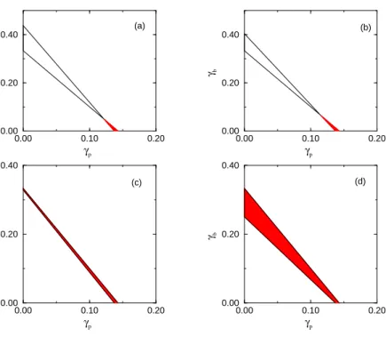
21 γb≤0. (55) This particular case was presented in Fig. 2, for each of the intervals Ii, just to illustrate the general discussion
we will present below. In this figure, the shaded regions, for each of the4peaks ofp4(E), indicate pairs of values of
(γp, γb)compatible with the conditions imposed by
inequal-ities (49) and (55). They represents the values of(∆p,∆b)
for which we cannot guarantee (based on logical arguments and restrictions as the ones deduced above) that the model is not critical. From now on we will call them “critical re-gions” in the parameter space. For all values ofi we ob-serve that there is a small shaded region, which shows us
that there is a non-zero, but small, probability of having crit-icality, in the physically accessible range of the parameter
α. That probability decreases asiincreases, since the prob-ability that a stable site becomes unstable is higher for larger value ofi.
From figures 2a and 2b, we see that the values ofγb
as-sociated with the shaded area (the values ofγp andγp for
which the model is possibly critical) are very small.γbis
re-lated to the size of the gaps between the peaks. That means that, to allow criticality,p4(E)∼pu(E)and very far from
the expectedp(E)forα≈0.25. In figures 2c and 2d, the values ofγbare a bit larger, but still not compatible with the
0.00 0.10 0.20 γp
0.00 0.20 0.40
0.00 0.10 0.20 γp
0.00 0.20 0.40
0.00 0.10 0.20 γp
0.00 0.20 0.40
γb
0.00 0.10 0.20 γp
0.00 0.20 0.40
γb
(a) (b)
(c) (d)
Figure 2. The parameter space ofpq(E), withq = 4in terms ofγp = ∆p/Ecandγb = ∆b/Ec. The shaded regions correspond to limited regions by the interception betweenα ≤1/4and7γp+ 3γb ≤1. Depending on the value ofEc−αE+
, there are 4 (q = 4) cases: (a)Ec−αE+ǫ[0,∆
p]; (b)Ec−αE+ǫ[∆p+ ∆b,3∆p+ ∆b]; (c)Ec−αE+ǫ[3∆p+ 2∆b,5∆p+ 2∆b]; e (d)Ec−αE+ǫ
[5∆p+ 3∆b,7∆p+ 3∆b].
In the case of a genericqwe can state that:
a) there is no value ofqsuch that the lines, that limit the critical regions, coincide, since the coefficients ofγb, for the
lines corresponding to inequalities (49) and (54), never have identical values;
b) for anyi≤q, there is always a region, in the param-eter space, for which the model may be critical. This can be proved with the same argument employed in item a).
c) the smaller the value ofi, the smaller the region, in the parameter space, for which the model may be critical; for the highest value ofi,i=q, the shaded areaAq decreases with
qaccording to a power law given by
Aq =
1
2(q−1)(2q−1) −
2(q−1)
(2q−1)(2q2−2q+ 1) =
= 1
2(q−1)(2q2−2q+ 1). (56)
Moreover,
lim
q→∞Aq = limq→∞
1
2(q−1)(2q2−2q+ 1) = 0. (57)
d) For any q > 2, the lines that define the region, in
the parameter space, where we cannot exclude the critical behavior, intercept each other fori < q−1.
In order to see that, we compare inequalities (49) and (54). The lines intercept when
(2q−1)(q−1)
q[(i−1)2+q(q−1)] >
1
q−1. (58) This expression can be re-written in the following form:
qi2−2qi−q3+ 4q2−3q+ 1<0. (59) Solving this equation forigives
i±= 1±
√
D
2q , (60)
whereD = 4q(q3−4q2+ 4q−1). Forq = 1we have
D = 0, soi=q= 1; forq= 2, it follows thatD <0, so there is no value ofisuch that the lines intercept each other. Forq > 2, we see thatD > 0, what means that there is some value ofisuch that the lines intercept each other. i−
is always smaller than1. In this case, it is easy to prove, by contradiction, thati+< q−1.
In order to argue that the OFC model indeed organizes itself towards criticality (regardless of whether it is critical or not), they calculated the branching rate and compared the behavior of both OFC and R-OFC models. They revisited Lise-Jensen’s approach, but now without assuming that
hEj+i=hEi+i=hE+i. (61) Instead, they estimated a recursion relation connecting the average energy of active sites between two successive gen-erations in an avalanche, at the beginning of the organization process. With this approach they were able to get, for the R-OFC model, better fittings for the average energy of active
sites,hE+iand, as a consequence, obtained also better
re-sults for the branching rateσ, versus the dissipation parame-terα(than the one obtained with Lise-Jensen approximation (61)).
We think that, even if we assume (61), what is reason-able for the stationary state, the use of a better approxima-tion for the energy distribuapproxima-tionp(E), like the one suggested by us (see (28)), will also led to better fittings for bothhE+i
andσversusα. In the particular case ofi =q- when the probability of having criticality is greatest (see figure 2d) -the expression (38) becomes
⌋
yi=q= 2|Ec(1−α)−[(2q−1)∆p+ (i−1)∆b]2|, (62)
and the solutions (37) can be rewritten as hE+iq(+)=
½
(Ec−E∗)/α, ifα <1−(Ec/E∗)
(Ec+E∗)/(2−α), ifα >1−(Ec/E∗) , (63)
hE+iq(−)= ½
(Ec+E∗)/(2−α), ifα <1−(Ec/E∗)
(Ec−E∗)/α, ifα >1−(Ec/E∗) , (64)
whereE∗= (2q−1)∆
p+ (q−1)∆q.
Analogously, the expressions for (33) become
σ(+)q =
½
0, ifα <1−(Ec/E∗)
2q[E∗−E
c(1−α)]/∆p(2q−1)α(2−α), ifα >1−(Ec/E∗) , (65)
σ(q−)=
½
2q[E∗−E
c(1−α)]/∆p(2q−1)α(2−α), ifα <1−(Ec/E∗)
0, ifα >1−(Ec/E∗) . (66)
⌈
Examining theses expressions we notice that they also do not increase linearly withα, as in what was called “ Lise-Jensen approximation” in [15]. We think that this is an evi-dence that, if we defineσas a function ofσi, we also would
obtain, forσ×α, a curve much closer to the simulation re-sults obtained by Miller and Boulter [15].
V
Conclusions
In this paper, we discuss the importance, to the analysis of random versions of models with self-organized criticality, of the the branching rate approach introduced in ([4]). We review the branching rate approach and we calculate, in de-tail, the exponentτthat characterizes the probability distri-bution of avalanche sizes. The result obtained, τ = 3/2, corroborates the connection between random SOC models and branching processes.
We concentrate our attention in the R-OFC model,
gen-eralizing our previous results to systems with an arbitrary connectivityq. Our calculations made clear how sensitive the results, to the approximation made for the energy distri-bution, necessary to calculate the branching rateσ.
We were also able to show that, for the more realistic ap-proximation to the energy distributionpq(E)in the
station-ary state (p(E)is approximated byqsquare peaks) there is only a small region of parameter space,∆p×∆b, for which
we cannot exclude criticality in the non conservative case. However, the values ofγp andγb for which our simplified
pq(E)is close to the distribution obtained from numerical
simulations do not belong to those regions.
Appendix
In that appendix we prove that ifi < q, the solutions of (47) are such thatαc >1/qorαc <0. In other words, we
must assumei=qin order to haveαc∈[0,1/q].
Dem] The solutions of (47) are given by
αc= −2i(2q−1)±
√
D
4q[(i−1)(i−2q) +q(q−1)], (67) withD = 4i2(2q−1)2+ 16q(2q−1)[(i−1)(i−2q) +
q(q−1)]. Then, under the assumptioni < q, and setting ⌋
(i−1)(i−2q) +q(q−1) = i2−2qi−i+ 2q+q2−q=
= (q−i)2+ (q−i)>0. (68) we get√D >2i(2q−1). This relation guarantees that, if one solution is negative, the other is positive.
Suppose now that the positive solution,αc>0, is such thatαc≤1/q; soα2c ≤1/q2. Then the inequality can be written
as follows:
b2α2c+b1αc+b0≤
b2
q2 +
b1
q +b0. (69)
Using equation (47), (69) is then
b2+qb1+q2b0≥0. (70)
Putting the coefficients (48) into (70) leads to
b2+qb1+q2b0 = 2q[(i−1)2+q(q−1)−(2q−1)(i−1) +i(2q−1)−q(2q−1)] =
= 2q[(i−1)2+q(q−1)−(2q−1)(q−1)] =
= 2q[(i−1)2−(q−1)2]≥0 (71) It is easy to see that, wheni < q, we have a contradiction. Therefore, fori < q,αc<0orαc>1/q. ✷
⌈
References
[1] P. Bak, C. Tang, and K. Wiesenfeld, Phys. Rev. Lett.59, 381 (1987); P. Bak, C. Tang, and K. Wiesenfeld, Phys. Rev. A38, 364 (1988).
[2] D. Dhar and R. Ramaswamy, Phys. Rev. Lett. 63, 1659 (1989); D. Dhar, Phys. Rev. Lett.64, 1613 (1990).
[3] A. Vespignani and S. Zapperi, Phys. Rev. Lett. 78, 4793 (1997); A. Vespignani and S. Zapperi, Phys. Rev. E57, 6345 (1998).
[4] S. Lise and H. J. Jensen, Phys. Rev. Lett.76, 2326 (1996).
[5] H-M. Br¨oker and P. Grassberger, Phys. Rev. E 56, 3944 (1997).
[6] M-L. Chabanol and V. Hakim, Phys. Rev. E 56, R2343 (1997).
[7] S. T. R. Pinho, C. P. C. Prado, and O. Kinouchi, Physica A 257, 488 (1998).
[8] O. Kinouchi, S. T. R. Pinho, and C. P. C. Prado, Phys. Rev. E 58, 3997 (1998).
[9] O. Kinouchi and C. P. C. Prado, Phys. Rev. E59, 4964 (1999). [10] L. Pietronero, A. Vespignani, and S. Zapperi, Phys. Rev. Lett.
72, 1690 (1994).
[11] Z. Olami, H. J. S. Feder, and K. Christensen, Phys. Rev. Lett. 68, 1244 (1992).
[12] R. Burridge and L. Knopoff, Bull. Seimol. Soc. Am.57, 341 (1967).
[13] J. X. de Carvalho and C. P. C. Prado, Phys. Rev. Lett. 84, 4006 (2000).
[14] S. Lise and M. Paczuski, Phys. Rev. E63, 036111 (2001).
[15] G. Miller and C. J. Boulter, Phys. Rev. E66, 016123 (2002).
[16] K. Christensen, Self-organization in models of sandpiles, earthquakes and flashing fireflies, PhD Thesis, (University of Aarhus, Denmark, 1992).
[17] S. Zapperi, K. B. Lauritsen, and H. E. Stanley, Phys. Rev. Lett.75, 4071 (1995).
[18] T. E. Harris,The Theory of Branching Processes, (Dover Pub-lications, New York, 1989).
[19] D. Dhar and S. N. Majumdar, J. Phys. A23, 4333 (1990).
[20] S. A. Janowsky and C. A. Laberge, J. Phys. A 26, L973 (1993).