Statistical-Thermodynamical Foundations
of Anomalous Diusion
Damian H. Zanette
Consejo Nacional de Investigaciones Cientcas y Tecnicas Centro Atomico Bariloche and Instituto Balseiro
8400 Bariloche, Ro Negro, Argentina
Received 07 December, 1998
It is shown that Tsallis's generalized statistics provides a natural frame for the statistical-thermodynamical description of anomalous diusion. Within this generalized theory, a maximum-entropy formalism makes it possible to derive a mathematical formulation for the mechanisms that underly Levy-like superdiusion, and for solving the nonlinear Fokker-Planck equation.
I Introduction: Diusion
pro-cesses
Among the elementary processes that underly natural phenomena, diusion is certainly one of the most ubiq-uitous. In an ensemble of moving elements {atoms, molecules, chemicals, cells, or animals{ each element usually performs, at a mesoscopic description level, a random path with sudden changes of direction and ve-locity. As a result of this highly irregular individual mo-tion, which is microscopically driven by the interaction of the elements with the medium and of the elements with each other, the ensemble spreads out. At a macro-scopic level, this collective behavior is {in contrast with the individual microscopic motion{ extremely regular, and follows very well dened, deterministic dynamical laws. It is precisely this smooth macroscopic spreading of an ensemble of randomly moving elements that we associate with diusion.
One of the rst systematic observations of diusion was made by the botanist Robert Brown in 1828. He noticed that pollen particles dispersed in water exhibit a very irregular, swarming motion. In 1905, Einstein conjectured that this \Brownian motion" is due to the interaction of pollen with the water molecules and, in fact, proved that microscopic particles suspended in a liquid \perform movements of such magnitude that they can be easily observed in a microscope, on account
of the molecular motions of heat" [1]. Since then, Brow-nian motion is used as a synonym of diusion.
A very suitable and very useful mathematicalmodel for Brownian motion is provided by random walks [2]. In its simplest version, a random walker is a point par-ticle that moves on a line at discrete time steps t. At each step, the walker chooses to jump to the left or to the right with equal probability, and then moves a xed distance x. This stochastic process can be read-ily generalized, rstly, by allowing the walker to move in a many-dimensional space. In addition, time can be made continuous by associating a random duration with each jump or by introducing random waiting times between jumps. Finally, the length of each jump can be also chosen at random from a continuous set with a prescribed probability distribution.
Suppose that the random walk is dened in contin-uous time and space, with a waiting time probability distribution () and such that the probability that the walker jumps from any pointrtor+xis p(x)dx.
The normalization of probabilities imposes Z
1 0
()d = 1; Z
p(x)dx= 1: (1) If, moreover, () andp(x) satisfy
c
hi= Z
1 0
()d <1; hx 2
i= Z
x 2
p(x)dx<1; (2)
d (xjxj) it can be proven thatP(r;t) obeys the diu-sion equation [2]
@P @t
=D r 2 r
P ; (3)
where D /hx 2
i=hi is the diusion constant, or diu-sivity. This equation has to be solved for a given initial condition P(r;0) with suitable boundary constraints. The densityn(r;t) of an ensemble of noninteracting dif-fusing particles obeys the same equation.
A typical solution to the diusion equation describes a density prole that, as time elapses, is smoothed out and broadens. In fact, it can be straightforwardly shown from the general solution that the width of the spatial distribution grows with time as
hr 2
i= Z
r 2
P(r;t)dr= 2dD t; (4) wheredis the space dimension. Correspondingly, it can be shown that the mean square distance between the present position and the initial position of a random walk that satises Eq. (2) is proportional to time. This proportionality between mean square displacement and time is the ngerprint of diusion, as it can be used ex-perimentally, numerically, and theoretically to detect this kind of transport mechanism in a given natural process.
Though, being a form of transport, diusion is inherently a nonequilibrium process, the large-time asymptotic dynamics of an ensemble of diusing par-ticles can be described in the frame of equilibrium sta-tistical mechanics. In fact, it is expected that, for very large times, the system reaches a state of thermody-namical equilibriumwith the medium {and between the particles, if they interact. In such state, the diusing
particles and the medium participate of a balanced in-terchange of momentum and energy, which mantains the particles in their characteristic irregular motion. Once this situation is reached, a connection between the parameters that characterize thermodynamical equilib-rium and particle dynamics should exist. Einstein in-vestigated this problem in 1905 [1], and concluded that diusivity and temperature are proportional:
D=k
B
T: (5)
Herek
B is Boltzmann constant, and
is the mobility. The mobility is dened as the inverse of the friction co-ecent, in the present case, of the diusing particles in the medium [4]. The Einstein relation, Eq. (5), pro-vides thus the expected connection between diusion and thermodynamical equilibrium.
of this paper is to review this generalization, comment-ing on some additional related topics brought to light in recent work.
II Anomalous diusion and
Levy ights
Any transport mechanism which, like diusion, behaves at mesoscopic level as an isotropic random process, but which violates Eq. (4), is generally refered to as anoma-lous diusion. More specically, most of the literature on anomalous diusion has been devoted to processes where the mean square displacement hr
2
i varies with time as
hr 2
i/t 2=z
; (6)
where z (6= 2) is the dynamic exponent, or random walk fractal dimension, of the transport process. Nor-mal diusion corresponds to z = 2. For z > 2, the growth rate of the mean square displacement is smaller than in normal diusion, and transport is consequently said to be subdiusive. On the other hand, for z <2 the mean square displacement grows relatively faster and transport is thus superdiusive. In the following, the attention will be mainly focused on this latter case.
II.1 Anomalous diusion in Nature
As advanced above, anomalous diusion occurs in a wide class of natural systems and processes. In the realm of physics, a paradigmatic example is given by particle transport in disordered media. Consider the motion of particles in a medium containing impurities, defects, or some kind of intrinsic disorder, such as in amorphous materials. Examples are disordered lattices, porous media, and dopped conductors and semicon-ductors. In these heterogeneous substrates, particles are driven by highly irregular forces, which determine a complex variation of the local transport coecients. This heterogeneity can in fact induce anomalous diu-sion. For instance, it has been experimentally shown that in quasi-one-dimensional ionic conductors such as hollandite (K1:54Mg0:77Ti7:23O16), where transport is very sensitive to the presence of impurities, the dynamic exponent is given by
z1 + 1
; (7)
with proportional to the temperature [6].
A reasonable model for transport in heterogeneous media is provided by a random walk in a lattice with quenched disorder [5]. This disorder applies to the depth of the potential wells at each lattice site, and to the potential barriers between sites. Randomness in these parameters induces a distribution for the time that the walker spends at each site before hoping to a neighbor. Generally, this waiting time distribution,
(), behaves as ()
,1,for
!1. For >1, the rst relation in Eq. (2) holds, and normal diusion is observed. On the other hand, for < 1 the mean waiting time diverges and diusion is anomalous. The corresponding dynamic exponent for 0<<1 is [7]
z= 2=(d>2); z= 2,d+d=(d<2): (8) A most important instance of anomalous diusion in physics occurs in turbulent ows. In fully developed turbulence, uid particles exhibit very irregular motion over a wide range of space and time scales. Based on empirical motivations, L. Richardson proposed in 1926 that the probabilityP(R;t) that two uid particles ini-tially close to one another have a separation Rat time tobeys the equation [8]
@P @t
= @ @R
D(R)
@P @R
; (9)
withD(r)R
4=3. Comparing with (3), it is clear that the Richardson equation is a diusion equation with space-dependent diusivity. Its solution immediately implies hR
2 i/ t
3, indicating that the relative motion of particles in fully developed turbulence corresponds to anomalous diusion with a dynamic exponentz= 2=3, which is well into the superdiusive regime.
Richardson's law has to be modied to take into account the fact that the vorticity eld in a turbulent ow is intermittent [9]. This means that vorticity {and, in particular, turbulent activity and dissipation{ is con-centrated on a relatively small volume in the whole sys-tem, which happens to be a fractal set. Experiments [10] suggest that the fractal dimension of this set is d
f = 2
:80:05. Incorporating this correction, it can be shown [11] thathR
2 i/t
12=(1+df), or z= 1 +
d f
A somewhat more abstract form of anomalous diu-sion is present in the evolution of chaotic Hamiltonian dynamical systems in phase space. Hamiltonian sys-tems are characterized by volume conservation in phase space, as stated by the Liouville theorem. The domain occupied by a given set of initial conditions in phase space can be strongly distorted under the eect of evo-lution, but its volume remains constant. Mechanical processes that preserve energy are instances of Hamilto-nian systems, but a huge host of systems {both continu-ous and discrete in time{ is known to belong to the same class. Since a single Hamiltonian system can exhibit both regular and chaotic evolution by simply chang-ing the initial condition, the dynamical geometry of its phase space is usually extremely intrincate. Zones of nested regular trajectories which alternate with chaotic regions are typically found at many scales, displaying selfsimilar structures. In the bulk of chaotic regions trajectories are extremely irregular and resemble ran-dom paths. On the other hand, when approaching the boundary with a regular region, the same trajectory can temporarily become much simpler and smoother. Con-sequently, as it evolves in phase space along a chaotic orbit, a Hamiltonian system alternates intermittently between zones of highly complex behavior and a regime of almost regular dynamics. Globally, this motion can be thought of as a stochastic process, and turns out to have the same statistical properties as anomalous dif-fusion.
A case studied in detail in the literature is the so-called Q-ow [12]. It is dened as a three dimensional velocity eld
_
x= @ =@y+sinz _
y= @ =@x+cosz _
z=
(11) with
(x;y) = k X j=1
cos[xcos(2 j=k) +ysin(2 j=k)]: (12) Here is a parameter and k is an integer that deter-mines the symmetry of the ow. The solution to Eqs. (11) is a complex trajectory that wanders in an in-nite connected net of channels of width of order , in-side which the trajectory looks like a random contour [13]. Numerical measurements of the statistical prop-erties of these diusion-like trajectories show that the
dynamic exponent z to be associated with them uc-tuates strongly as a function of [12]. For k= 6 and 0:8<<1:8,z varies in the interval
1<z<2; (13) making apparent that the motion is supperdiusive, as in turbulence. Anomalous diusion has also been ob-served in dissipative (non-Hamiltonian) dynamical sys-tems, both in simulations and in experiments. For ex-ample, a dynamic exponentz1:2 has been measured in the Taylor-Couette ow[14].
As stated in the Introduction, anomalous diusion is not restricted to physical systems. This kind of trans-port has in fact been detected to underly several biologi-cal processes. Some sectors of genomic DNA sequences, for instance, are known to exhibit statistical properties analogous to anomalous diusion. To stress this corre-spondence, \DNA walks" have been dened [15]. DNA, which codes genetic information, is a large molecule in the form of a chain of nucleotides. Each nucleotide con-tains either a purine or a pyramidine base. Two purines {the adenine (A) and the guanine (G){ and two pyra-midines {the cytosine (C) and the thymine (T){ are in turn present in the DNA chain. Therefore, the informa-tion code in DNA is a symbolic chain of four letters: A, C, G and T. Amazingly, within DNA only a small por-tion does code informapor-tion for protein building (3% in the human genome) whereas other zones are noncoding, their specic role being unknown. A one-dimensional DNA walk is constructed by sequentially running over the chain of nucleotids. Each time a purine is found the walker jumps rightwards, whereas when a pyramidine is found the jump occurs leftwards. For instance,
A less involved instance of anomalous diusion in biology appears in the ight patterns of certain birds. In particular, it has been found [17] that in the foraging behavior of the wandering albatross (Diomedea exulans) the ight-time intervals exhibit a power-law distribu-tion. This results in a anomalous diusive-like motion which, according to eld measurements on the Bird Is-land, South Georgia, has a dynamic exponent z1:2. The kind of ight patterns observed in these seabirds is supposed to reect a complex structure in the under-lying ecosystem, especially, in the spatial distribution of the exploited environment. It has been suggested that albatrosses specialize in long journeys of random foraging, searching for patchily and unpredictably dis-persed prey over several million square kilometers. As discussed in the next section, anomalous diusion is in-herently related with fractal geometry, scale-invariance, and self-similarity, which in the present example seem to drive the predator-prey dynamics.
Of course, the previous collection of examples of anomalous diusion in Nature is not at all exhaustive, but only pretends to give a hint on the variety of sys-tems driven by this kind of transport. For a more detailed account, the reader is refered to the review by Bouchaud and Georges [5]. This review is also an excellent reference to the mathematical treatment of anomalous diusion, which is briey introduced in the following.
II.2 Random-walk models of anomalous
diu-sion
In view of the ecacy of random walks in modeling normal diusion at a mesoscopic level, it is desirable to nd a similar stochastic model describing anoma-lous diusion. It has already been mentioned in Section II.1 that introducing a waiting time distribution which, for large waiting times, behaves as ()
,1,with <1, produces the anomalousdynamicexponent given in Eq. (8). In this case z>2 and, therefore, transport is subdiusive. Note that the source of anomalyin these random walks is the divergency of the average waiting timehi. For<1, the long-tailed distribution () allows for very long waiting times with relatively high probability, violating thus the rst relation in Eq. (2). These long waiting times produce an overall reduction
of eciency in the transport mechanism with respect to normal diusion, and leads to subdiusive behavior. Taking into account the previous argument, in can be expected that the violation of the second of relations (2) will lead, on the other hand, to superdiusion. In fact, having a divergent mean square displacementhx
2 i requires the jump probability distributionp(
x
) to have a long tail for large x, in a sense to be made precise immediately. This long-tailed distribution would pro-duce, with relatively high probability, very long jumps. Globally, this transport mechanism should result more ecient than normal diusion, and superdiusive be-havior is expected.It can be easily shown that, ind-dimensional space, the mean square displacement diverges if
p(
x
) 1 xd+ (14)
for large x, with <2. Note that, for such distribu-tion, normalization requires >0. It is therefore to be expected that a random walk with a jump distribution p(
x
)x,d, with 0
< <2 does not model normal diusion, but some kind of superdiusive motion. Of course, a large score of functions satisfy Eq. (14), and are thus candidates to play the role of a jump distri-bution for a superdiusive random walk. Among them, Levy distributions have been studied in detail.
Levy distributions [18] are dened through their Fourier transform, which reads
p(
k
) = Zexp(i
k
x
)p(x
)dx
= exp(,bk )c
p 1(
k)p 2(
k) = exp(,b 1
k )exp(
,b 2
k
) = exp[ ,(b
1+ b
2) k
] = p
3(
k): (16)
d Levy functions are not the only stable distributions, the Gaussianp(x)/exp(,x
2) being probably the best-known example. The (one-dimensional) Cauchy distri-bution, p(x) / (1 +x
2),1, is another instance. Sta-ble distributions play a fundamental role in probability theory since according to the central limit theorem { which is usually stated for the Gaussian function{ the addition of random variables tends to one such distribu-tion. In particular, as P. Levy demonstrated through his generalization of the Gaussian central limit theo-rem [18, 19], adding random variables with a power-law distribution as in (14) {whose second momenthx
2 i diverges for <2{ leads asymptotically to a Levy dis-tribution.
Another important property of Levy distributions, which is reected in its power-law large-x asymptotic behavior, Eq. (14), is the absence of characteristic length scales. This implies that random walks with Levy jump distributions have self-similar properties. In particular, it can be shown that the set of points vis-ited by this kind of random walk is a fractal of dimen-sion [20]. As a consequence, these distributions are ubiquitous in the realm of self-similarity geometry {the geometry of fractals.
A discrete-time random walk whose jump distribu-tion is given by a Levy funcdistribu-tion as in Eq. (15) is called a Levy ight. It has been suggested [21] that the Fourier transformP(k;t) of the probability distribution of nd-ing the walker at a given point at time t satises the evolution equation
@P @t
(k;t) =,D
k
P(k;t): (17) This equation generalizes, in the Fourier representation, the diusion equation (3). A straightforward dimen-sionality analysis shows that the anomalous diusivity isD
/b=t, where tis the time step of the random walk. In free space, equation (17) can be readily solved:
P(k;t) =P(k;0)exp(,D
k
t): (18)
For a delta-like initial condition, P(r;0) = (r), one hasP(k;0) = 1 and, thus,
P(r;t) = (2) ,d
Z
exp(,ikr,D
k
t)dk: (19) This function remains unchanged, except for a constant factor, if both space and time are conveniently rescaled, P(
1=
r;t) = ,d=
P(r;t). Using this scale invari-ance, one can write
P(r;t) =t ,d=
(r =t 1=
); (20)
where is a function of a single variable [22]. In turn, this implies
hr 2
i/t 2=
; (21)
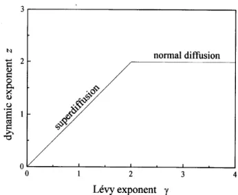
for 0<<2. This result, which has been here derived for a delta-like initial distribution, can be generalized by simple superposition to more general initial conditions. It shows that a Levy ight with 0< <2 represents superdiusion with a dynamic exponent z = . On the other hand, for power-law jump distributions with > 2 the dynamic exponent corresponds to normal diusion,z= 2 (Figure 1).
Figure 1. The diusion dynamic exponentz as a function
of the Levy exponent.
The fact that in Levy ights the mean square dis-placement hx
2
contrast with Eq. (21){ that the mean square displace-ment of the walker after a certain time is, on the aver-age over innitely many realizations, also innite. The arguments used to derive Eq. (21) are therefore of lim-ited validity [21, 22], and have to be takencum grano salis. The result (21) is expected to be valid for nite times, i.e. in a certain portion of the whole random walk, and on averages over a nite number of trajecto-ries. The same result would be valid during a certain time if the jump distribution p(x) is a Levy function in some (large) range of values of x, but has a cuto for sucently large x[23]. In spite of this drawback, Levy ights provide a very powerful tool for model-ing superdiusion because of the mathematical proper-ties of the Levy distributions, summarized above. They are thus a very satisfactory starting point as a model for studying the statistical mechanics of superdiusive transport, generalizing the results outlined in the In-troduction for normal diusion.
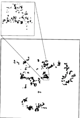
Figure 2. The rst 104 points visited by a two-dimensional
random walk generated by a power-law jump distribution with exponent = 1:5, starting at the center of the main
frame. The amplication illustrates the self-similar proper-ties of this process.
Before passing to the discussion of superdiusion in a statistical-mechanical frame, a comment is in order on the numerical simulation of superdiusive random walks. Due to the cumbersome properties of Levy dis-tributions in real space [20], it is not convenient {in nu-merical calculations{ to work directly with these func-tions. Rather, power-law distributions with the same asymptotic properties as Levy's, Eq. (14), are used. For instance, one can take
p(x) = N (1 +x)
d+
; (22)
with N a normalization constant. The Fourier trans-form of these distributions behaves precisely like a Levy distribution for smallk,p(k)1, bk
. Also, they show the same scale invariance for largex, wich leads to self-similar properties in the associated random walks. In Figure 2 the rst 104 points visited by a random walk in two dimensions, with the jump distribution given in (22) and = 1:5, are shown. Note the clustered, fractal-like structure of this set of points.
III Maximum-entropy
formal-ism for anomalous diusion
Entropy plays a central role in the foundations of equi-librium and nonequiequi-librium statistical mechanics. It is well known from the work by L. Boltzmann and others that entropy provides a natural link between nonequi-librium processes and their asymptotic states of ther-modynamical equilibrium. In addition, the whole the-ory of equilibrium statistical mechanics can be derived from a variational formalism for the entropy, as follows. Dene the entropy S as a functional of the probability distributionp
i over the states
iof a given system, S[p] =,k
B X
i p
iln p
i
; (23)
wherek
B is Boltzmann constant. Find then the values of p
i that maximize
S[p], taking into account the nor-malization constraint, P
i p
i = 1, and {if required by particular conditions of the system under study{ any additional constraint on p
i. The value of p
i resulting from this maximization procedure gives the probability of nding the system in state iwhen thermodynamical equilibrium has been reached. For instance, introduc-ing the canonical constraintP
i
p i=
energy of stateiandEis the thermodynamical energy, the maximization of entropy produces the well-known Boltzmann distributionp
i
/exp(, i) [4].
III.1 Traditional formalism
As a starting point for including normal diusion in the frame of equilibrium statistical mechanics, the procedure of entropy maximization has been applied to obtain the jump probability distribution p(
x
) in a discrete-time random walk [24]. In this case, entropy is dened as a straightforward generalization of (23),S[p] =,k B
Z
p(
x
)ln[ dp(
x
)]dx
: (24) Here is a characteristic length, whose meaning will become clear immediately. The distribution p(x
), in fact, has units of length to the power ,d. The maxi-mization of S[p] is carried out taking into account the normalization ofp(x
),Z
p(
x
)dx
= 1; (25) and imposing the additional constraintZ x
2
p(
x
)dx
= 2d; (26)
which is inspired in the second relation of Eq. (2). Ex-cept for a dimensionality factor,
2 is thus the mean square displacement associated withp(
x
).Under these conditions, the maximization of en-tropy yields
p(
x
) = (2 2),d=2
exp(,x 2
=2 2
); (27) namely, a Gaussian jump distribution. Since, in view of the constraint (26), the mean square displacement as-sociated withp(
x
) is nite, the maximum-entropy for-malism applied as above to the jump distribution of a random walk describes normal diusion.The question on whether anomalous diusion can be derived from a variational formalism for the entropy arises now quite naturally. Montroll and Shlesinger [24] have shown that this is in fact possible, but requires re-placing the constraint (26) by a more complex condition onp(
x
). In particular, Levy ights, Eq. (15), are ob-tained from the maximization of the entropy (24) if the jump distribution satises, along with normalization,c Z
ln
(2) ,d
Z
exp(,i
k
x
,bk )d
k
p(
x
)dx
= constant: (28)d This is however a quite unsatisfactory answer to the above question. Indeed, besides its complexity, the constraint (28) is anything but a natural condition to impose to the jump distribution. In Montroll and Shlesinger's words, \it is dicult to imagine that any-one in an a priori manner would introduce" such a condition for maximizing the entropy with respect to p(
x
). This remark would at once exclude Levy ights {and anomalous diusion with them{ from the frame of the maximum-entropy formalism and, therefore, from a natural connection with equilibrium statistics.In Ref. [25], a dierent approach has been proposed to tackle the problem of deriving anomalous diusion from the maximization of entropy. Since replacing the constraint on the jump distribution implies imposing unconventional, forced conditions on p(
x
), a possibleway out is to replace the form of the entropy instead. In particular, it has been found that the form of the entropy proposed by Tsallis [26, 27] produces, upon maximization with the constraints prescribed by this generalized theory, power-law jump distributions with the asymptotic behavior given in (14). As described in the following, random-walk models of anomalous diu-sion nd thus a natural statistical-mechanical basis in Tsallis' theory.
III.2 Generalized formalism
maximization procedure. For a system whosei-th state is occupied with probabilityp
i, the generalized entropy reads
S q[
p] =, 1, P i p q i 1,q
; (29)
where qis a real parameter. For the canonical ensem-ble, where the energy of the i-th state is
i and the average energy is E
q, the generalized constraint to be imposed top
i, along with probability normalization, is X i i p q i = E q : (30)
In this generalized formalism, in fact, the average of any observable O is dened as hO i
q = P i O i p q i. This average is usually refered to as theq-expectation value ofO[28].
The generalized statistical-mechanical formalism based on Eqs. (29) and (30) has some remarkable properties. First of all, it reduces to the traditional Boltzmann-Gibbs formulation in the limit q ! 1. In fact, Eq. (23) is recovered from (29) in that limit ex-cept for the factork
B, which has here been convention-ally put equal to unity. The canonical constraint (30) reduces in turn to the traditional denition of mean en-ergy. The new formalism preserves the full Legendre-transformation structure of thermodynamics for all q [27], leaving invariant in form the main results of statis-tical thermodynamics, such as the Ehrenfest theorem, the H-theorem, the von Neumann equation, the Bo-golyubov inequality, and the Onsager reciprocity theo-rem [28]. Its seems to be particularly useful in dealing with systems involving long-range correlations and non-extensivity, as the formalism itself is non-extensive for q6= 1. The Tsallis exponentqhas thus been interpreted as a measure of non-extensivity. Since its introduction a decade ago [23] Tsallis statistics has found successful applications to a large class of problems of high interest, ranging from gravitational systems, to turbulent ows, to optimization algorithms. Many of these applications are described in detail in other papers of the present issue, and are therefore no longer discussed here.
In order to apply Tsallis statistics to discrete-time random walks in the spirit outlined in the previous sec-tion, Eqs. (24) and (26) have to be generalized accord-ing to (29) and (30), respectively. As a function of the jump probability, the generalized entropy can be
writ-ten as [23, 25, 29]
S q[
p] =, 1 1,q
1, ,d Z d p(x)
q
dx
; (31) whereas the canonical constraint transforms into a con-dition on the q-expectation value ofx
2: hx 2 i q = ,d Z x 2[
p(x)] q
dx= 2
: (32)
Here, preserves its identication as a typical length associated with the jump probability. However, for q6= 1,
2does not coincide with the mean square length of the jumps. For simplicity, the dimensionality factor in the right-hand side of Eq. (26) has now been ab-sorved by .
It is shown in the following that the maximizationof S[p] as dened in (31) with the constraints (25) and (32) {which, as in the case of the traditional formalism, is carried out by the standard method of Lagrange multi-pliers [26, 27]{ produces a power-law jump distribution. The exponent of the power-law depends on the space dimension and on the Tsallis exponent q. This jump distribution is not a Levy distribution like (15), but has the same type of asymptotic behavior, Eq. (14). For suitable values of d and q, this form of p(x) will therefore dene a random walk with anomalous prop-erties.
For the sake of clarity, the results in one dimension are shown rst [23, 29]. The jump distribution resulting from the maximization procedure is, in this case,
p(x) =Z ,1 q
1,(1,q)x 2
1=(1,q )
(33) where the partition functionZ
q is given by Z q = Z +1 ,1
1,(1,q)x 2
1=(1,q )
dx: (34) The positive constant is one of the Lagrange multi-pliers, which can be expressed as a function ofusing the constraint (32), as shown below. In the generalized formulation of statistical mechanics is related to the temperatureT in the standard form, /1=T.
c
p(x) = r
(q,1)
, 1 q ,1
,
1 q ,1
, 1 2
1 +(q,1)x 2
,1=(q ,1)
(35) for 1<q<3, and
p(x) = 8 > < > :
q (1,q )
,(
1 1,q
+ 3 2) ,(
1 1,q
+1)
1,(1,q)x 2
1=(1,q )
ifx 2
< 1 (1,q )
;
0 otherwise (36)
forq<1. For q!1, of course, the Gaussian (27) is reobtained. Note that the Tsallis exponent qis related to the exponent in Eq. (14) according to [25]
= 3 ,q q,1 or
q= 3 + 1 +
: (37)
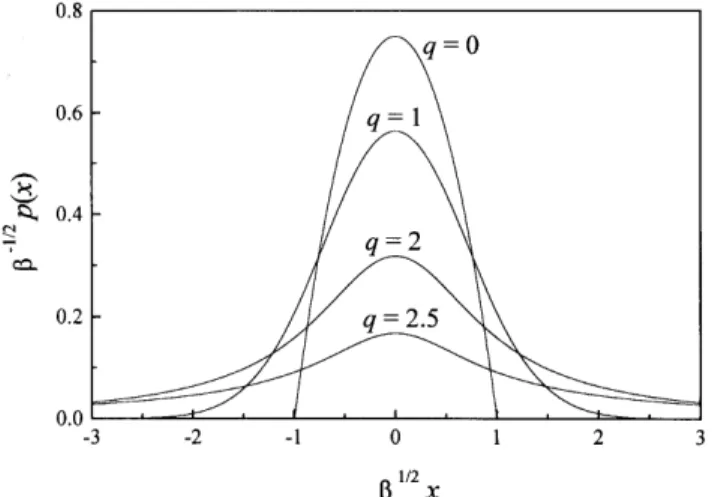
Figure 3 shows the prole of p(x) for several values ofq. d
Figure 3. Jump probability distribution derived from Tsal-lis statistics, for some values of the TsalTsal-lis exponentq. For q = 1 the standard Gaussian is obtained. Note the cut-o
for q <1, and the long-tailed power-law distributions for q>1.
Regarding anomalous diusion, thus, it is clear that the case q < 1 is irrelevant. In fact, for such val-ues of the Tsallis exponent p(x) exhibits a cut-o at jxj= 1=
p
(1,q), and vanishes for largerjxj, as shown by Eq. (36). This implies at once that the mean square displacement associated with p(x) is nite and the re-sulting random walk corresponds to normal diusion. The attention is consequently focused in the following on the case 1<q<3, Eq. (35). In this case, the mean
square displacement is
hx 2
i= 8 < :
[(5,3q)] ,1 if
q<5=3,
1 ifq5=3:
(38) Therefore, for 1 < q < 5=3 1:67 the mean square displacement is still nite, and the random walk corre-sponds to normal diusion. On the other hand, anoma-lous superdiusion is obtained for 5=3q<3.
It is interesting to calculate now the q-expectation value ofx
2 which, in the frame of Tsallis statistics, re-places {as an average quantity{ the mean square dis-placement of the standard formulation. According to the constraint (32) imposed top(x) in the maximization of entropy, thisq-expectation value should be nite. In fact,
hx 2
i q = 12
2 4
r (q,1)
2
, 1 q ,1
,
1 q ,1
, 1 2
3 5
2(q ,1)=(3,q ) ; (39) for 1<q<3. The fact that, in contrast with the mean square displacement, hx
2 i
q is nite, seems to indicate that the constraint (32) is a natural one in the frame of anomalous-diusion random walks [25]. Note moreover that Eq. (39) along with (32) gives the connection be-tween the Lagrange multiplier and the characteristic length,
/
,2
Equations (35) and (36) make clear that, as stated above, the maximization of entropy within Tsallis' for-malismdoes not lead to Levy distributions for the jump probability. Rather, a plain power-law function of the jump lengthxis obtained. Levy distributions are how-ever reobtained when considering the temporal evolu-tion of the random walk generated byp(x). In fact, the displacementr of the walker aftert time steps is given by the sum of the successive jumps. By virtue of the generalized central limit theorem [18, 19] discussed in Section II.2 the probability distributionP(r;t) is thus given, for largetand <2 (i.e. q5=3), by a stable Levy distribution with Levy exponent . For > 2, on the other hand, the usual form of the central limit theorem holds and the total displacement distribution is a Gaussian. The dynamic exponentz of the random walk { which coincides with for < 2 (see Section II.2) { is then
z= 8 < :
2 ifq<5=3, (3,q)=(q,1) ifq5=3:
(41) This connection between the dynamic exponent and the Tsallis exponent q { which is illustrated by the curve d = 1 in Figure 4 { constitutes indeed the main re-sult of the description of anomalous diusion in the frame of the Tsallis' formulation. It shows that a close relation exists between the properties of a Levy-ight process and the non-extensiveness of the involved statis-tics. As far as the underlying statistical frame diers from Boltzmann-Gibbs', the maximum-entropy formal-ism produces a random walk which models superdiu-sion as a Levy ight.
As in the case of the jump distribution, the total mean square displacement hr
2
i associated with Levy ights diverges. On the other hand, theq-expectation value ofr
2is well dened for all relevant
q(1<q<3), cf. Eq. (39). This can be calculated taking into ac-count the scaling properties of P(r;t), Eq. (20), and reads
hr 2
i q =
8 < :
D(q) ,1
t
(3,q )=2 if
q<5=3, D(q)
,1 t
q ,1 if
q5=3:
(42) The proportionality factorD(q) depends onqonly. In-terpreting now the Lagrange multiplieras the inverse of the temperature {as prescribed in the frame of Tsal-lis thermodynamics [27]{ the above equation can be
seen as a generalization of the Einstein relation (5) [30]. Equations (4) and (5) imply in fact thathr
2 i/
,1 tfor normal diusion, and Eq. (42) is the extension of this result to Tsallis statistics. Again, the fact thathr
2 i
q is nite for Levy ights suggests that Tsallis' formalism provides a natural frame for the statistical description of such kind of anomalous diusion.
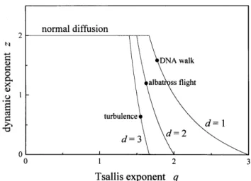
Figure 4. The diusion dynamic exponentzas a function of
the Tsallis exponentq, for dierent spatial dimensions. The
dots stand for some of the instances of anomalous diusion discussed in Section II.1.
Though the algebra is more involved than above, anomalous diusion in more than one dimension can be straightforwardly treated in the frame of Tsallis statis-tics, and the main conclusions are qualitatively the same as for the one-dimensional case. Maximazing the entropy given in (31) in the d-dimensional space pro-duces formally the same jump distribution as in (33), where the partition function has however to be calcu-lated as ad-dimensional integral. The jump probability can be normalized if
q< 2 +d
d
; (43)
and the associated mean square displacement is nite if
q< 4 +d 2 +d
: (44)
c
z= 8 < :
2 ifq<(4 +d)=(2 +d),
2=(q,1),d if (4 +d)=(2 +d)<q<(2 +d)=d:
(45)
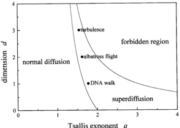
d This connection is represented graphically in Figure 4.
Figure 5. Phase diagram in the (q ;d)-plane, displaying the
zones of normal and anomalous diusion, and the forbid-den region where the jump probability distribution cannot be normalized. The dots stand for some of the instances of anomalous diusion discussed in Section II.1.
IV Nonlinear diusion and
Tsallis statistics The diusion equation,
@P @t
=D r 2 r
P ; (46)
which governs the evolution of the probabilityP(r;t)dr of nding a Brownian particle in a neighborhooddr of pointrat timet, can be generalized to take into account additional mechanisms acting on both the microscopic dynamics of the particle and the mesoscopic dynamics of an ensemble of such particles. A rather straightfor-ward generalization introduces for instance the eect of an external force eld, F(r;t), acting on each particle [3, 31]. This force eld enters the diusion equation as a drift term, namely,
@P @t
=,r r
(FP) +D r 2 r
P : (47)
This equation, which combines the eect of probability drift {due to the force{ and of probability spreading { due to diusion{ can be seen to govern a huge class of random processes, in a generic space of statesr[3, 31]. It is generally refered to as the Fokker-Planck equation. Further generalizations, mainly justied on a phe-nomenological basis, have lead to propose a nonlinear version of the Fokker-Planck equation [32], namely,
@P @t
=,r r
(FP ) +
D r 2 r P
; (48)
where >0 and are suitable real constants. With-out loosing generality, one can x = 1, by chang-ing P
! P and = ! . In such case, Eq. (48) can be phenomenologically interpreted as a Fokker-Planck equation where, if 6= 1, the diusion coe-cent depends on the probabilityP(r;t). This density-dependent diusivity represents nonlinear eects aris-ing, for instance, from interaction between the diusing particles. Such kind of nonlinearities have been ob-served in several real processes, such as transport in porous media (2) [33], surface growth (= 3) [34], liquid lm spreading under gravity ( = 4) [35], and Marshak radiative heat transfer ( = 7) [36], among others [37].
force. This problem has recently been treated by Tsal-lis himself [40] and, in an alternate form, by Compte and Jou [41].
Consider then the one dimensional version of Eq. (48) for the probability densityP(x;t),
@P @t
=, @ @x
[F(x)P ] +
D @
2 P
@x
2
; (49)
with x r, and with F(x) = k 1
,xk
2. This
time-independent, linear form of the drift force corresponds, in general, to a quadratic potential {i.e. an Ornstein-Uhlenbeck random process [3]{ whereas it reduces to a linear potential {namely, a constant force{ for k
2= 0. For== 1, this equation can be straightforwardly solved, for instance, by Fourier-Laplace transforming. A special solution is
c
P(x;t) = 1 Z(t) exp
(t)[x,x(t)] 2
; (50)
where
(t) (0) =
Z(0) Z(t)
2
= [(1,)exp(,2k 2
t) + ] ,1
(51) with = 2D (0)=k
2, and
x(t) =+ [x(0),]exp(,k 2
t) (52)
d with=k
1 =k
2. This particular solution has the impor-tant property that, fort!0 and(0)!1, it reduces to a delta-like distribution,P(x;0) =[x,x(0)]. Since Eq. (49) is linear for== 1, and delta distributions can be used as a base for the space of initial conditions P(x;0), a suitable linear combinationof functions of the form (50) provides the solution to the linear equation for any initialcondition in that space. In this sense, (50) gives the general solution to the linear Fokker-Planck equation with the above prescribed drift force.
Focus now the attention on the functional form of the particular solution to the linear problem given in Eq. (50). As a function of x, P(x;t) is a Gaussian, essentially of the same type as (27). The dierences are, rstly, that the spatial coordinate x is shifted by an amount x(t). The Gaussian is therefore centered around a position which depends on time. Secondly, the width of the Gaussian, which is proportional to
,1=2, depends also on time. Since the solution (50) preserves normalization, the normalization factorZ
,1 is time-dependent.
The Gaussian prole of P(x;t) in Eq. (50) sug-gests that this solution can be formally derived from a suitably extended maximum-entropy formalism, in its standard Boltzmann-Gibbs version. In fact, it can be shown [40] that such form of P(x;t) derives from the
maximization of S[P] =
Z +1 ,1
P(x;t)lnP(x;t)dx; (53) with the extended constrains
Z +1 ,1
P(x;t)dx= 1; (54) Z
+1 ,1
[x,x(t)]P(x;t)dx= 0; (55)
and Z
+1 ,1
[x,x(t)] 2
P(x;t)dx= 1 2(t)
; (56)
for arbitrary x(t) and (t). The special forms of these functions that make the probability distribution satisfy the linear Fokker-Planck equation can be obtained by simply replacingP(x;t) in the equation.
It should be by now clear that one is immediately interested at which solutions are obtained if, instead of the standard maximization principle, the Tsallis' for-malism is used. Namely, take the generalized entropy
S q[
P] =, 1 1,q
1,
Z +1 ,1
P(x;t) q
dx
; (57)
and maximize it with respect to P(x;t) imposing the generalized constrains
Z +1 ,1
[x,x(t)]P(x;t) q
and Z +1 ,1
[x,x(t)] 2
P(x;t) q
dx= 1 2(t)
: (59)
This produces [40]
P(x;t) = 1 Z
q( t)
1,(t)(1,q)[x,x(t)] 2
1=(1,q ) ; (60) to be compared with Eq. (33). Remarkably enough, this form of P(x;t) turns out to be a solution to the one-dimensional nonlinear Fokker-Planck equation for the linear drift force if
q= 1 +,; (61)
and
(t) (0) =
Z
q(0) Z
q( t)
2
: (62)
As for Levy-ight anomalous diusion, P(x;t) can be normalized only ifq <3. This denes a forbidden re-gion for>2 + (Fig. 8).
The functionZ q(
t) is explicitely given by
Z q(
t) =Z q(0)[(1
,
q)exp(
,t=) + q]
1=(+) ; (63) with
q = 2
D (0)Z q(0)
, k
2
; (64)
and ==k 2(
+). The function x(t) is the same as for the linear case, Eq. (52). Note that the normaliza-tion constraint, Eq. (54), has not been imposed in the maximization of S
q[
P]. In fact, the preservation of the norm of P(x;t) is now not compatible with the other two constraints. Rather, it turns out that the integral of the probability density over the whole space varies with time according to
Z +1 ,1
P(x;t)dx=
Z q(
t) Z
q(0)
,1 Z
+1 ,1
P(x;0)dx: (65) This implies that the norm is conserved for all times only if = 1, or if
q = 1 {when Z
q does not depend on time. If q
>1 the norm monotonically increases for >1 and decreases for <1. If
q
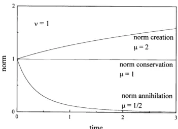
< 1, on the other hand, the opposite behavior is observed. More-over, for<0 the norm diverges or vanishes at a nite time. Figure 6 illustrates these dierent regimes for = 1 and some values of.
Figure 6. Evolution of the norm in the solutions to the non-linear Fokker-Planck equation for= 1 and some values of . These curves correspond to
q >1.
The case of constant force,k
2= 0, can be analyzed as the suitable limit of the above solution fork
2 !0. In particular, taking exp(,t=)1,t= in Eq. (63) it is found that
Z q(
t) =Z q(0)
1 + 2(+)
D (0)Z q(0)
, t
1=(+)
: (66) In this limit,the width of the distribution {which is pro-portional to
,1=2{ exhibits a well-dened power-law dependence on time. In fact, according to Eq. (62), (t)
,1=2 / t
=(+). This makes possible to assign a dynamic exponent to this kind of diusion, given by
z= 1 +
: (67)
Figure 7. Evolution of the width in the solutions to the non-linear Fokker-Planck equation for= 1 and some values of . For the case of \negative diusivity,"= 1=2.
Figure 8. Phase diagram in the (;)-plane, displaying the
dierent regimes of anomalous diusion and norm evolution in the solutions to the nonlinear Fokker-Planck equation. In the forbidden region the probability distribution cannot be normalized.
Equation (61) makes evident that the non-extensivity inherent to Tsallis statistics is related, in the frame of its application to the resolution of the nonlin-ear Fokker-Planck equation (49), to the nonlinnonlin-earity of the equation itself. This nonlinearity translates, at the level of the solutions, into anomalous properties of the involved transport processes. Thus, a clear connection between anomalous diusion and the non-extensivity of the underlying statistics arises again. It is impor-tant to point out that, in contrast with Eq. (50), the solutions (60) to the nonlinear Fokker-Planck equation derived from Tsallis' formalism cannot be combined to give a general solution. In fact, due to the nonlinear-ity of Eq. (49), no superposition principle holds, and
(60) are particular solutions for special initial condi-tions only. Nevertheless, the straightforward way in which these solutions have appeared as an extension of the linear case along the lines of Tsallis' generalization, reinforces strongly the close relation between Tsallis' formalism an anomalous diusion.
V Conclusion
Though normal diusion is ubiquitous in Nature, a large {and still growing{ class of real systems is driven by a dierent kind of transport processes, namely, by anomalous diusion. In view of the current importance of many of these systems {which range from turbulent ows, to disordered media and chaotic dynamics, to ight patterns in birds{ it is of high interest having at hand a formulation able to place anomalous diusion in a statistical-thermodynamical frame, generalizing thus Einstein's theory for normal diusion. However, within Boltzmann-Gibbs statistics \the wonderfull world of clusters and intermittencies and bursts that is associ-ated with Levy distributions would be hidden from us if we depended on a maximum entropy formalism that employed simple traditional auxiliary conditions" [24]. It has been here shown that, instead, Tsallis general-ized statistics is a strong candidate to succesfully yield such a formulation.
Tsallis statistics provides a natural frame for the mathematical foundations of anomalous diusion in two forms. In the rst place, jump distributions of random-walk models for Levy-like superdiusion can be straightforwardly derived from a maximum-entropy principle within the generalized theory. In fact, such distributions exhibit power-law long tails, which are an essential feature in the results of the theory. At once, Tsallis statistics furnishes an elegant explanation for the appearence of Levy distributions in other nat-ural phenomena, as the result of the superposition of random variables with long-tailed distributions. In the second place, the functional form of the distributions resulting from Tsallis' formalism successfully suggests the solution to the nonlinear Fokker-Planck equation, which describes both subdiusion and superdiusion.
still wait to be treated in the frame of the generalized statistics. For instance, it would be important to ex-tend the derivation of random-walk models of anoma-lous diusion to the case of subdiusion. As explained in Section II, this requires introducing suitable waiting-time densities. Since power-law functions can fulll this role, Tsallis statistics is again a natural stating point to derive such densities. Another extension would re-gard diusion processes on fractals. In fact, Levy-like diusion anomalies are the consequence of mechanisms driving the dynamics of the diusing particles. An al-ternative formulation, which is relevant to many appli-cations, takes into account that such anomalies orig-inate rather in the complex geometry of the medium where particles diuse. The connection between frac-tal geometry and Tsallis statistics has been identied early, and it can thus be expected that diusion on frac-tal substrates nds a satisfactory statistical-mechanical frame in such theory. Finally, it would be interesting to descend a level further in the dynamicalbases of anoma-lous diusion, and try to apply Tsallis' formalismto the formulation of deterministic mechanical approaches to this kind of transport.
As a nal remark it is worth mentioning that, very recently, Tsallis' formalism has been improved by re-dening the normalization ofq-expectation values [42]. This has solved, in a single step, two main drawbacks of the theory. In fact, in its original formulation, Tsal-lis statistical mechanics is not invariant under energy shifts, and the q-expectation value of a constant de-pends on the state of the system under study. Although the correction to the theory does not involve important changes in the qualitative results, it represents a major improvement from a formal viewpoint. Here, Tsallis statistics has been applied to anomalous diusion in its original form. A relevant step forward would be to reanalyze this process in the frame of the corrected theory.
Acknowledgements
Fruitful discussions with P.A. Alemany and C. Tsallis are acknowledged. G. Drazer contributed some valuable remarks on the manuscript. The author is grateful to Fundacion Antorchas, Argentina, for nancial support.
References
[1] A. Einstein, Ann. Phys.17, 549 (1905).
[2] E.W. Montroll and B.J. West, inFluctuation Phenom-ena, E.W. Montroll and J.L. Lebowitz, eds. (Elsevier, Amsterdam, 1979) p. 61.
[3] N.G. van Kampen,Stochastic Processes in Physics and Chemistry(North-Holland, Amsterdam, 1992).
[4] R. Kubo, Statistical Mechanics (North-Holland, Ams-terdam, 1988).
[5] J.-P. Bouchaud and A. Georges, Phys. Rep. 195, 127
(1990).
[6] J. Bernasconi, H. Beyelev, S. Straessler and S. Alexan-der, Phys. Rev. Lett.42, 819 (1979).
[7] J. Machta, J. Phys. A18, L531 (1985).
[8] L.F. Richardson, Proc. Roy. Soc. London, Ser. A110,
709 (1926).
[9] B.B. Mandelbrot, J. Fluid Mech.62, 331 (1974).
[10] R.A. Antonia, N. Phan-Thien and B.R. Satyoparakash, Phys. Fluids24, 554 (1981).
[11] M.F. Shlesinger, B.J. West and J. Klafter, Phys. Rev. Lett58, 1100 (1987).
[12] G.M. Zaslavsky, R.Z. Sagdeev, and A.A. Chernikov, Sov. Phys. JETP67, 270 (1988); A. A. Chenikov, B. A.
Petrovichev, A. V. Rogalsky, R. Z. Sagdeev and G. M. Zaslavsky, Phys. Lett. A144, 127 (1990).
[13] M.F. Shlesinger, G.M. Zaslavsky and J. Klafter, Nature
363, 31 (1993).
[14] E.R. Weeks, T.H. Solomon, J.S. Urbach and H.L. Swin-ney, in Levy Flights and Related Topics in Physics, M.F. Shlesinger, G.M. Zaslavsky, and U. Frisch, eds. (Springer, Berlin, 1995) p. 51.
[15] C.-K. Peng, S.V. Buldyrev, A.L. Goldberger, S. Havlin, F. Sciortino, M. Simons and H.E. Stanley, Nature356,
168 (1992).
[16] H.E. Stanley, S.V. Buldyrev, A.L. Goldberger, S. Havlin, R.N. Mantegna, C.-K. Pend, M. Simons and M.H.R. Stanley in Levy Flights and Related Topics in Physics, M.F. Shlesinger, G.M. Zaslavsky, and U. Frisch, eds. (Springer, Berlin, 1995) p. 331.
[17] G.M. Viswanathan, V. Afanasyev, S.V. Buldyrev, E.J. Murphy, P.A. Prince, H.E. Stanley, Nature 381, 413
(1996).
[18] P. Levy, Theorie de l'addition des variables aleatoires
(Gauthier-Villars, Paris, 1937).
[19] A. Araujo and E. Gine,The Central Limit Theorem for Real and Banach Valued Random Variables(Wiley, New York, 1980).
[20] B.D. Hughes, M.F. Shlesinger, and E.W. Montroll, Proc. Acad. Sci. USA78, 3287 (1981).
[21] A. Compte, Phys. Rev. E53, 4191 (1996).
[23] C. Tsallis, A.M.C. Souza, and R. Maynard, in Levy Flights and Related Topics in Physics, M.F. Shlesinger, G.M. Zaslavsky, and U. Frisch, eds. (Springer, Berlin, 1995) p. 269.
[24] E.W. Montroll and M.F. Shlesinger, J. Stat. Phys.32,
209 (1983).
[25] P.A. Alemany and D.H. Zanette, Phys. Rev. E49, 956
(1994).
[26] C. Tsallis, J. Stat. Phys. 52, 479 (1988).
[27] E.M.F. Curado and C. Tsallis, J. Phys. A 24, L69
(1991) [corrigenda24, 3187 (1991);25, 1019 (1992)].
[28] C. Tsallis, Chaos, Solitons & Fractals6, 539 (1995).
[29] C. Tsallis, R.M. Maynard and A.M.C. de Souza, Phys. Rev. Lett.75, 3589 (1995).
[30] D.H. Zanette and P.A. Alemany, Phys. Rev. Lett.75,
366 (1995).
[31] H.S. Wio, An Introduction to Stochastic Processes and Nonequilibrium Statistical Physics(World Scientic, Singapore, 1994).
[32] A formal derivation of the nonlinear Fokker-Planck equation from a Langevin equation within the frame of Tsallis statistics has recently been proposed in L. Bor-land, Phys. Rev. E57, 6634 (1998).
[33] M. Muskat,The Flow of Homogeneous Fluids Through Porous Media (McGraw-Hill, New York, 1937); P.Y. Polubarinova-Kochina, Theory of Ground Water Move-ment(Princeton University Press, Princeton, 1962). [34] H. Spohn, J. Phys. (France) I3, 69 (1993).
[35] J. Buckmaster, J. Fluid Mech.81, 735 (1977).
[36] E.W. Larsen and G.C. Pomraning, SIAM J. Appl. Math.39, 201 (1980).
[37] W.L. Kath, Physica D12, 375 (1984).
[38] J.D. Murray, Mathematical Biology (Springer, Berlin, 1989).
[39] J.R. King, J. Phys. A 23, 3681 (1990); D.H. Zanette,
J. Phys. A26, 5339 (1993).
[40] C. Tsallis and D.J. Bukman, Phys. Rev. E 54, R2197
(1996).
[41] A. Compte and D. Jou, J. Phys. A29, 4321 (1996).