ISOTROPIC WORK SOFTENING MODEL FOR FRICTIONAL GEOMATERIALS: DEVELOPMENT BASED ON LADE AND KIM CONSTITUTIVE SOIL MODEL
Kuo-Hsin Yang
Dept. of Civil Engineering, The University of Texas at Austin, Texas, Austin, USA Christianne de Lyra Nogueira
Dept. of Mine Engineering, Universidade Federal de Ouro Preto, MG, Brazil Jorge G. Zornberg
Dept. of Civil Engineering, The University of Texas at Austin, Texas, Austin, USA
Abstract: An isotropic softening model for predicting the post-peak behavior of frictional geomaterials is presented. The proposed softening model is a function of plastic work which can include all possible stress-strain combinations. The development of softening model is based on the Lade and Kim constitutive soil model but improves previous work by characterizing the size of decaying yield surface more realistically by assuming an inverse sigmoid function. Compared to original softening model using the exponential decay function, the benefits of using the inverse sigmoid function are highlighted as: (1) provide a smoother transition from hardening to softening occurring at the peak strength point, and (2) limit the decrease of yield surface at a residual yield surface, which is a minimum size of yield surface during softening. The proposed softening model requires three parameters; each parameter has it own physical meaning and can be easily calibrated by a triaxial compression test. Data from triaxial compression testing on Monterey No. 30 sand is applied to demonstrate the calibration procedure and examine the variation of model parameters with different loading conditions. Results show all parameters are highly correlated to confining pressures. The proposed softening model can provide a useful tool for evaluating those structures on which the post-peak behavior of frictional materials should be emphasized, e.g. earth structures under large loading or deformation conditions or the structures having an intensive soil-structures interaction, etc.
Keywords: Lade and Kim soil model; Softening function; Post-peak behavior; Frictional Geomaterial
XXIX CILAMCE
1. INTRODUCTION
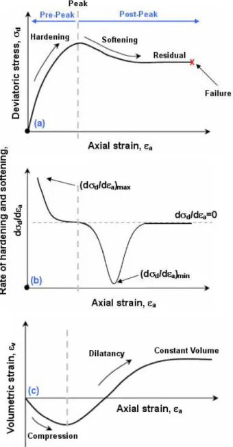
The terminology of soil “softening” is referred to, after soil reaches peak strength, the soil strength would decrease with the increasing deformation. This softening behavior can be often observed from conventional laboratory tests, specifically for triaxial test (Lade and Prabucki 1995; Chu et al.1996; Yoshida and Tatsuoka 1997; Suzuki and Yamada 2006, etc.). Figure 1a illustrates a typical stress-strain behavior of frictional soil under triaxial compression. Strain hardening is developed initially and then strain softening after deviatoric stress reaches peak value. The strain softening will cease at residual value. The stress state reaches residual strength is also called critical state by some researchers. The soil specimen will eventually “fail” at large soil strain. In Fig. 1b, the rate of changing deviatoric stress with axial strain is close to zero at peak strength then gradually decreases to a minimum negative value during softening and slowly increases back to zero again. Figure 1c shows the corresponding volumetric strain behavior. The volumetric compression and dilatancy occurs during shearing and then the dilatancy will level out at a constant volumetric strain.
Beside the observation in laboratory, the softening behavior is also often noticed in the field for earth structures under large loading and deformation conditions or the structures having an intensive soil-structures interaction; for example, landslide, foundation and platform, soil anchors, soil piles and Geosynthetic-Reinforced Soil (GRS) structures (e.g.
Murff 1980; Huang et al. 1994; Leschinsky 2001; Liu et al. 2004;Hsu 2005; Troncone 2005;
etc.). Numerical methods have been frequently adopted to study the behavior of earth structures in soil under various loading conditions. The merit of numerical analyses mainly include the relatively low-cost, less labor and capability of reduplication compared to physical tests; however, the interactive behavior between an earth structure and soil is difficult to analyze accurately by a simple numerical model. The soil constitutive model used to analyze an earth structure’s behavior in frictional soil is often considered as a nonlinear elastic model:
e.g. Duncan hyperbolic model (Duncan and Chang 1970), elastic-perfectly plastic model: e.g.
Mohr- Coulomb model, and an elastoplastic model: e.g. Hardening Soil model (Schanz 1999) and Lade and Kim soil model (Kim and Lade 1988; Lade and Kim 1988a, 1988b and 1995; Lade and Jakobsen 2002) etc. Although those models have their own specialties for analyzing specific problem; the natures of strain softening and volumetric dilatancy of frictional soil are usually not taken into account.
Among aforementioned models, Lade and Kim soil constitutive model (Kim and Lade 1988; Lade and Kim 1988a,1988b and 1995; Lade and Jakobsen 2002) equips both work hardening and softening model and has been applied to model the behavior of soils or rocks in numerous researches (e.g. Lee et al. 2002; Borja 2004; Baxvanisetal et al. 2006). A review of Lade and Kim model is provided in Section 2 and Appendix A. In Lade and Kim model, the soil hardening and softening behavior is modeled by an isotropic inflation and deflation of yield surface which is governed by hardening and softening laws. The hardening and softening laws are function of plastic work Wp. Lade and Kim argued that the advantages of
using plastic work characterizing yield behavior is because it does not involve tests with complicated stress-paths and it also avoids difficulties in determination of yield points on stress-strain curves. In addition, computation of plastic work is straight forward and the plastic work appears to capture yielding in terms of shear strains as well as volumetric strains. They also claimed that the evaluation of the yield criterion was performed in the hardening regime where the soil behavior has been studied experimentally and is reasonably well known. However, actual movement and shape of yield surface in the softening regime is much less known; therefore in Lade and Kim soil model, the decrease of yield surface is just simply assumed as an exponential decay function.
2. REVIEW OF LADE AND KIM SOIL MODEL
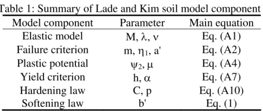
Lade and Kim (or called single hardening) constitutive soil model (Kim and Lade 1988; Lade and Kim 1988a, 1988b and 1995; Lade and Jakobsen 2002) is an elastoplastic model composed by following components: elastic model, failure criterion, plastic potential function for non-associated flow rule, yield criterion, isotropic hardening and softening models. The formulation is developed based on numerical experimental data sets of testing frictional materials under various loading conditions. The model incorporates thirteen parameters and all can be determined using data from isotropic compression and triaxial compression tests. Table 1 summarized the model components, parameters and main governing equations in the latest version of Lade and Kim soil model (Lade and Jakobsen 2002). A brief review of the framework and the components are provided in Appendix A. Readers are recommended referring to Lade and Jakobsen (2002) for other details. This section will focus on introducing the softening model in Lade and Kim soil model.
Table 1: Summary of Lade and Kim soil model component Model component Parameter Main equation
Elastic model M, λ, ν Eq. (A1) Failure criterion m, η1, a' Eq. (A2)
Plastic potential ψ2, μ Eq. (A4) Yield criterion h, α Eq. (A7) Hardening law C, p Eq. (A10)
Softening law b' Eq. (1)
2.1 Softening Model in Lade and Kim Soil Model
The softening model is one of two components of isotropic yield function (Eq. (A6)) in Lade and Kim soil model. As discussed in Section A.4, the yield function describes the shape and size of yield surface; the shape of yield surface is governed by yield criterion fp’(σ) in Eq. (A7) and the increasing and decreasing size of yield surface is controlled by hardening and softening law fp’’(Wp), respectively. Hardening law is introduced in Section A.5 and softening
law will be discussed in this section.
For soil during hardening, as the plastic work increases, the isotropic yield surface inflates until the current stress point reaches the peak failure surface or stress level S=1. The relation between the increasing yield surface fp’’and plastic work Wp (normalized by atmospheric pressure pa) is described by a monotonically increasing function whose slope decrease with
increasing plastic work, as shown in Fig. 2. After stress state reaches peak failure surface, the soil behavior changes from hardening to softening. During soil softening, the increase of plastic work will case the deflation of yield surface. The yield surface is assumed deflating isotropically according to an exponential decay function:
a p p BW
p Ae
f
−
=
′′ (1)
in which A and B are positive constants to be determined on the basis of the location and slope of the hardening curve at S=1.
1 S p BW
p a
p e f A
=
⎥ ⎥ ⎦ ⎤ ⎢
⎢ ⎣ ⎡
′′
1 S p a p
p
f 1 ) p / W ( d
f d b B
= ⎥ ⎥ ⎦ ⎤ ⎢
⎢ ⎣ ⎡
′′ ′′ ′
= (3)
In which both the size of the yield surface fp’’ and the derivative d fp’’/d (Wp /pa) are obtained from the hardening curve at S=1. The value of d fp’’ is negative during softening. The only
parameter in softening model is b’, which is a positive value (b′≥0). The b’ parameter value equal to zero corresponds to a perfect plastic material. The effect of b’on softening curve is illustrated in Fig.2.
Figure 2: Modeling of work hardening and softening (Lade and Jakobsen 2002)
3. PROPOSED SOIL SOFTENING MODEL
Base on the general observation of soil post-peak behavior stated in Section 1 and the experience of using and calibrating the softening model in Lade and Kim soil model, it is found that the size of decaying yield surface is more like an inverse sigmoid curve rather than an exponential decay curve. This will be demonstrated using the data from three triaxial compression tests in Section 4. Figure 3 illustrate the inverse sigmoid function used for proposed softening model. The improvement of predicting softening behavior by using inverse sigmoid function is highlighted in following two factors:
1. Provide a smoother transition from hardening to softening at the peak strength point. The abruptly transition observed in Fig. 2 indicates a suddenly rate changing form hardening to softening at peak strength point; this doesn’t agree with the observation in Fig 1b which shows the rate changing from hardening to softening is gradually at peak strength point.
as shown in Fig 1b, the stress state should stay at a residual strength when soil experiences large deformation. This can be simulated by the model parameter fpr’’ in
proposed softening model.
Figure 3: Proposed softening model based on inverse sigmoid function
The governing equation is expressed as:
⎪⎭ ⎪ ⎬ ⎫ ⎪⎩
⎪ ⎨ ⎧
⎥ ⎥ ⎦ ⎤ ⎢
⎢ ⎣ ⎡
⎟⎟ ⎠ ⎞ ⎜⎜ ⎝ ⎛ − −
+ − ′′ = ′′
= =
1 S a
p
a p 1
S p p
p W
p W b exp a c
1 )
f (
f (4)
where (fp’’)S=1 is the size of yield surface at peak condition and (Wp/pa)S=1 is the value of
normalized plastic work at peak condition which can be evaluated from the hardening curve at
S=1. a, b and c are all positive real numbers: a controls the magnitude of softening curve; b
controls the curvature of softening curve; and c controls the vertical distance of softening curve. a, b and c can be calibrated from a triaxial compression test. c is calculated as:
pr 1 S
p) f
f (
1 c
′′ − ′′ =
=
(5)
where fpr’’ is the yield function on residual condition which can be obtained by substituting the stress components at residual stress state into Eq. (A7). a, b and fpr’’ are three parameters for
the proposed softening model. In addition, when the normalized plastic work starts at (Wp/pa)S=1, the size of yield surface (fp’’)(Wp/pa)S=1 calculated by Eq. (4) would differ from
(fp’’)S=1 by 1/(c+a) (indicated in Fig.3). Preliminary study shows c is usually negligible
compared to parameter a and the discontinuity between (fp’’)S=1 and (fp’’)(Wp/pa)S=1 can be
hardening and softening curves, the value of this gap (i.e. 1/a) is recommend less than 5% of (fp’’)S=1.
An incremental form of the new softening model is also provided for the calculation of plastic modulus H and the implementation into a finite element program, such as ABAQUS (ABAQUS 1995) and PLAXIS (2005), through a user-defined material module.
2 1 S a p a p 1 S a p a p a p p p W p W b exp a c p W p W b exp ab ) p W ( d f d ⎥ ⎥ ⎦ ⎤ ⎢ ⎢ ⎣ ⎡ ⎪⎭ ⎪ ⎬ ⎫ ⎪⎩ ⎪ ⎨ ⎧ ⎥ ⎥ ⎦ ⎤ ⎢ ⎢ ⎣ ⎡ ⎟⎟ ⎠ ⎞ ⎜⎜ ⎝ ⎛ − − + ⎪⎭ ⎪ ⎬ ⎫ ⎪⎩ ⎪ ⎨ ⎧ ⎥ ⎥ ⎦ ⎤ ⎢ ⎢ ⎣ ⎡ ⎟⎟ ⎠ ⎞ ⎜⎜ ⎝ ⎛ − − − = ′′ = = (6)
4. CALIBRATION PROCEDURE
4.1 Properties of Test Soil
Data of triaxial compression testing on Monterey No. 30 sand (Li 2005) is selected to demonstrate the calibration procedure. Monterey No. 30 sand is a clean uniformly graded sand classified as SP in the unified system. The properties of Monterey No. 30 sand are listed in Table 2.
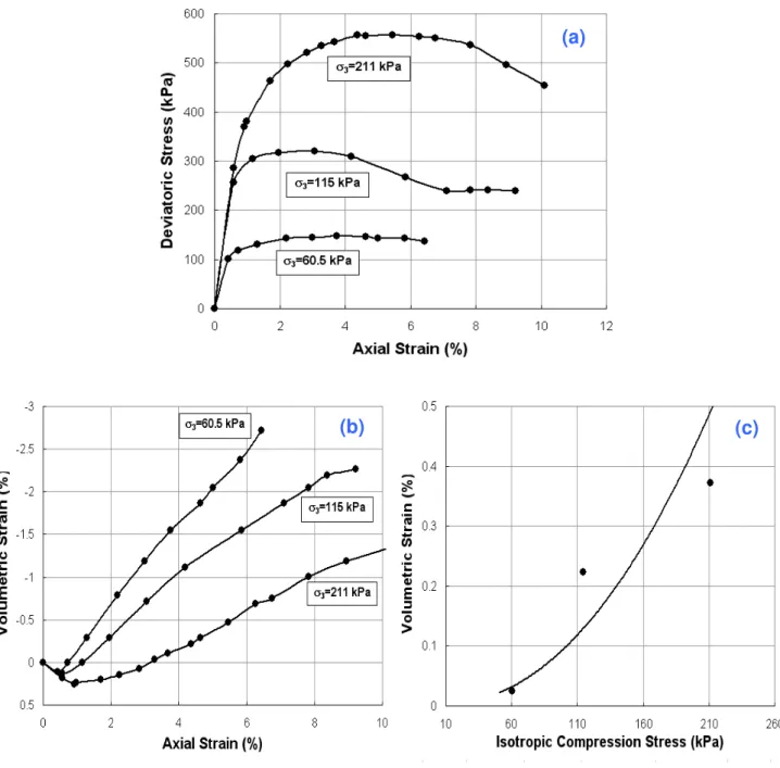
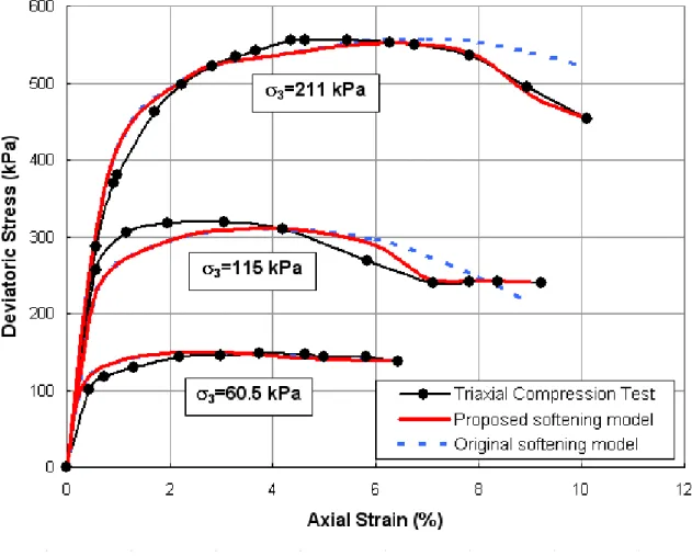
The specimen with relative density of 65% was tested under three confining pressures. Figure 4a shows the deviatoric stress and strain relations. A clear strength softening behavior in stress-train curve can be observed at larger confining pressure. Figure 4b shows the volumetric and axial strain relations. Figure 4c shows the isotropic compression and volumetric strain relations. Note the data in Fig. 4c is only for calibrating hardening parameters, C and p, and not necessary for the proposed softening parameters.
Table 2: The properties of Monterey No. 30 sand Soil Type Monterey No. 30 sand
D50 (mm) 0.4
Uniformity coefficient, Cu 3
Coefficient of gradation, Cz 1.1
Specific gravity, G 2.66
Soil classification SP
Max dry unit weight, γd,max (kN/m3) 16.70
Min dry unit weight, γd,min (kN/m3) 14.76
4.2Calibration Procedure
The step of calibration procedure is as follows:
1. For the calibration of all model parameters (expect for the softening parameters), select the data points until the peak strength point and follow the procedure addressed by Lade and Kim (Kim and Lade 1988; Lade and Kim 1988a,1988b). Obtain (fp’’)S=1 and (Wp)S=1
Figure 4: Triaxial compression test results: (a) deviatoric stress and axial strain; (b) volumetric and axial strain; (c) isotropic compression and volumetric strain
2. For the calibration of softening parameters, select the data points from the peak strength point to the last data point for each triaxial test. Calculate fp’’using equation Eq. (A7) and obtain softening parameter fpr’’ from the calculated fp’’ at the last data point.
3. Calculate Wp using following equation:
∑ σ ε +
= =
= =
j i
1
i p
1 S p
p (W ) d d
W (7)
where dσ and dεp are the incremental stress and plastic strains tensors. dεp can be calculated
by subtracting elastic strain increment from total strain increment, i is the number of increments of data points.
(a)
4. Calculate c using Eq. (5)
5. Plot the data points in following coordinates
1 S a p a
p p (W p )
W
X′= − = (8)
and
c f ) f (
1 Y
p 1 S p
− ′′ − ′′ = ′
=
(9)
The softening function in Eq. (4) is translated into
X b ae
Y′= − ′ (10)
Best fitting the plotted data points using an exponential function and obtain softening parameters a and b. Figures. 5 shows the best fitting curve and the obtained model parameters
a and b for three confining pressures. Table 3 shows the final calibrated parameters.
Y' = 1.8815e-54.348X' R2 = 0.9104
0 0.05 0.1 0.15 0.2 0.25
0 0.05 0.1 0.15
X'
Y'
(a) σ3 = 211kPa
Y' = 1.1045e-124.72X' R2 = 0.9979
0 0.01 0.02 0.03 0.04
0 0.02 0.04 0.06 0.08
X'
Y'
Y' = 0.7522e-165.41X' R2 = 0.7018
0 0.05 0.1 0.15 0.2
0 0.01 0.02 0.03
X'
Y'
(b) σ3 = 115kPa (c) σ3 = 60.5kPa
Table 3: Material parameters for Monterey No. 30 sand Model component Parameter Value Elastic model M, λ, ν 705, 0.257, 0.35 Failure criterion m,η1, a' 0.0214, 24, 0
Plastic potential ψ, μ -8.51, 2.4 Yield criterion h, α 0.67, 0.2 Hardening law C, p 5.07x10⁻⁵, 1.9 Softening law f''pr, a,b
Confining pressure 211kPa 85.68, 1.88, 54.3 115kPa 52.48, 1.10, 124.7 60.5kPa 50.13, 0.75, 165.4
Figures 6 show the correlations of calibrated softening parameters with confining pressures. Because frictional material does not have strength under unconfined condition, the regression line in Fig. 6a is forced to intercept at origin. Figures 6 show the softening model parameter are highly correlated to confining pressure.
R2 = 0.2323
0 10 20 30 40 50 60 70 80 90 100
0 50 100 150 200 250
σ3 (kPa)
fpr
''
(a) parameter fpr’’
R2 = 0.9969
0 0.2 0.4 0.6 0.8 1 1.2 1.4 1.6 1.8 2
0 50 100 150 200 250
σ3 (kPa)
a
R2 = 1
0 20 40 60 80 100 120 140 160 180
0 50 100 150 200 250
σ3 (kPa)
b
(b) parameter a (c) parameter b
Figures 7 show final results of calibration. The calibration curves using original softening model are also plotted for comparison. The calibration curves from original softening model are calculated by varying original softening parameter b’ until maximum correlation with the experimental data is found (i.e., maximum R2). As shown in Figs. 7, the calibration curves using original approach either overestimate the size of yield surface at last data point in Fig. 7a or underestimate that in Fig. 7b. It is fair to conclude that the new softening model based on inverse sigmoid function can depict the trend of experimental data better than original approach by exponential decaying function.
(a) σ3 = 211kPa
(b) σ3 = 115kPa (c) σ3 = 60.5kPa
5 COMPARE TO EXPERIMENTAL RESULTS
After the calibration of softening parameters, Lade and Kim soil model with the proposed softening model are used to predict stress-strain relation of Monterey No. 30 sand. The results of prediction are shown in Fig. 8. A modified forward Euler scheme with error control (Jakobsen and Lade, 2002) is adopted to integrate stress at each strain subincrement. In modified forward Euler scheme, the size of each strain subincrement is determined so that the new stress state fulfils the specified tolerance and only the absolutely necessary number of strain subdivision are applied. As demonstrate in a special example in Jakobsen and Lade (2002), they showed that with this integration scheme, the error can be suppressed under 10-4 approximately with a maximum number of subincrements of 30.
The prediction curves using original softening model are also plotted for comparison. Due to the over and under estimation of the sizes of yield surfaces in Figs. 7, the original softening model also shows an over and under estimation of prediction in Figs. 8. Figure 8 confirms the proposed softening model shows better prediction results. Figure 8 also shows that the proposed softening model can capture well different magnitudes of strength softening under different confining pressures. Last, because volumetric strain is computed by using plastic potential function in Eq. (A4), the difference between using proposed and original softening model to predict volumetric and axial strain seems slight; therefore, the results of predicting volumetric and axial strain are not presented herein.
6 CONCLUSIONS
This paper proposed an isotropic softening model for predicting the post-peak behavior of frictional geomaterials. The development of softening model was based on the Lade and Kim soil constitutive model but improved previous work by characterizing the size of decaying yield surface by using an inverse sigmoid function. The inverse sigmoid function more realistically captured the softening behavior in following twofold: (1) provide a smooth transition from hardening to softening occurring at the peak strength point, and (2) limit the decrease of yield surface until a residual yield surface. Three softening model parameters fpr’’, a and b could be easily calibrated by a triaxial test. The calibration produce was demonstrated by using the data of three triaxial compression tests on Monterey No. 30 sand. Results indicate three softening parameters were strongly correlated to confining pressures.
In future work, the proposed softening model can be implemented into a finite element program through a user-defined material module. This can provide a useful tool to numerically evaluate the structures on which the post-peak behavior of frictional material should be emphasized.
REFERENCES
ABAQUS. 1995. ABAQUS manuals version 5.5. Hibbit, Karlson and Sorensen Inc.
Baxevanis, T. Papamichos, E. Flornes, O. Larsen, I. 2006. Compaction bands and induced permeability reduction in Tuffeau de Maastricht calcarenite. Acta Geotechnica-Springer Verlag. vol. 1, n. 2, pp.123-135
Borja, R.I.. 2004. Computational modeling of deformation bands in granular media, II: Numerical simulations. Computer Methods in Applied Mechanics and Engineering. vol. 193, pp. 2699-2718.
Chu, J., Lo, S. and Lee, I.K. 1996. Strain softening and shear band formation of sand in multi-axial testing. Geotechnique, vol. 46, n. 1, pp. 63-82
Duncan, J. M., and Chang, C. Y. 1970. Nonlinear analysis of stress and strain in soils. Journal of the Soil Mechanics and Foundations Division, ASCE, vol. 96, n. SM5, pp. 1629-1653.
Huang, C., Tatsuoka, F., and Sato, Y.1994. Failure mechanisms of reinforced sand slopes loaded witha footing. Soils and Foundations. vol. 34 n.2, pp. 27-40.
Jakobsen KP and Lade PV. 2002. Implementation algorithm for a single hardening constitutive model for frictional materials. International Journal for Numerical and Analytical Methods in Geomechanics. 26: pp. 661-681.
Kim, M.K. and Lade, P.V. 1988. Single hardening constitutive model for frictional materials - I. Plastic potential function. Computers and Geomechanics, 5, pp. 307-324
Lade, P.V. and Kim, M.K. 1988a. Single hardening constitutive model for frictional materials II. Yield criterion and plastic work contours. Computers and Geomechanics, 6, pp. 13-29
Lade, P.V. and Kim, M.K. 1988b. Single hardening constitutive model for frictional materials III. Comparisons with experimental data. Computers and Geomechanics. 6, pp. 31-47.
Lade, P.V. and Prabucki, M.J. 1995. Softening and preshearing effects in sand. Soils and Foundations 1995; vol. 35 n. 4, pp. 93–104
Lee, D.H., Juang, C.H., Lin, H.M., and Yeh, S.H. 2002. Mechanical behavior of Tien-Liao mudstone in hollow cylinder tests. Canadian Geotechnical Journal, vol. 39, n. 3, pp. 744-756
Leschchinsky, D. 2001. Design dilemma: Use peak or residual strength of soil. Geotextiles and Geomembranes, vol. 19, n. 2, pp. 111-125
Li, C., 2005, Mechanical response of fiber-reinforced soil, Ph.D. dissertation, the University of Texas at Austin.
Liu, J., Xiao, H.B., Tang, J., and Li, Q.S. 2004. Analysis of load-transfer of single pile in layered soil. Computers and Geotechnics, vol. 31, n. 2, pp. 127-135
Murff, J.D. 1980. Pile capacity in a softening soil. International Journal for Numerical and Analytical Methods in Geomechanics, vol. 4, n. 2, pp. 185-189
PLAXIS. 2005. Plaxis Finite Element Code for Soil and Rock Analyses, Version 8.2, P.O. Box 572, 2600 AN Delft, The Netherlands (Distributed in the United States by GeoComp Corporation, Boxborough, MA).
Schanz, T., Vermeer, P.A., Bonnier, P.G., 1999. Formulation and verification of the Hardening-Soil Model. Beyond 2000 in Computational Geotechnics. Balkema, Rotterdam. pp. 281-290.
Suzuki, K and Yamada, T. 2006. Double strain softening and diagonally crossing shear bands of sand in drained triaxial tests. International Journal of Geomechanics, vol. 6, n. 6, pp. 440-446
Troncone, A. 2005. Numerical analysis of a landslide in soils with strain-softening behaviour
Geotechnique, vol. 55, n. 8, pp. 585-596
APPENDIX A
This appendix provides a brief review of the framework and the components of the Lade and Kim soil constitutive model. In order that the presentation follows a logic developmental sequence, the components are presented in the following sequence: elastic model, failure criterion plastic potential and flow rule, yield criterion and work hardening law.
A.1 Elastic Model
The elastic strain increments are calculated following Hook’s law. The Young’s modulus
E nonlinearly varies with stress state. The expression of Young’s modulus was derived based on the principle of energy conservation. According to this derivation, Young’s modulus can be expressed in following equation in term of a power law:
λ ⎥ ⎥ ⎦ ⎤ ⎢ ⎢ ⎣ ⎡ ′ ⎟ ⎠ ⎞ ⎜ ⎝ ⎛ ν − ν + + ⎟⎟ ⎠ ⎞ ⎜⎜ ⎝ ⎛ = a 2 2 a 1 a p J 2 1 1 6 p I Mp
E (A1)
where I1 is the first invariant of the stress tensor; J’2 is the second invariant of the deviatoric stress; and pa is the atmospheric pressure in the same unit as E and I1; M, λ, andPoisson’s
ratio ν are constant dimensionless material parameters, which can be obtained from simple tests such as triaxial compression tests.
A.2 Failure Criterion
A three-dimensional failure criterion is expressed in terms of the first I2 and third I3
invariant of the stress tensor:
m a 1 3 3 1 n p I 27 I I f ⎟⎟ ⎠ ⎞ ⎜⎜ ⎝ ⎛ ⎟ ⎟ ⎠ ⎞ ⎜ ⎜ ⎝ ⎛ −
= (A2)
and
1 n
f =η at failure (A3)
1
= η
n
f means current stress state reaches material peak failure surface. Another parameter a’
is required in order to include the effective cohesion and the tension which can be sustained by concrete and rock. A translation of the principal stress space along the hydrostatic axis is performed; thus, a constant stress a’pa is added to the normal stresses before substitution into Eq. (A2). The value of a’pa reflects the effect of the tensile strength of the material. The
parameters m, η1, and a’are constant dimensionless numbers, which may be determined from results of simple tests such as triaxial compression tests.
A.3 Plastic Potential and Flow Rule
μ ⎟⎟ ⎠ ⎞ ⎜⎜ ⎝ ⎛ ⎟ ⎟ ⎠ ⎞ ⎜ ⎜ ⎝ ⎛ Ψ − − Ψ = a 1 2 2 2 1 3 3 1 1 p p I I I I I
g (A4)
where I2 is the second invariant of the stress tensor. The material parameters ψ2and μ are dimensionless constants that may be determined from triaxial compression tests. The parameter ψ1is related to the curvature parameter m of the failure criterion as follows:
27 . 1 1 0.00155m
−
=
Ψ (A5)
A.4 Yield Criterion
The yield surface are associated with and derived from surfaces of constant plastic work, as explained by Lade and Kim (1988a). The isotropic yield function is expressed as follows:
0 ) W ( f ) ( f
fp = p′ σ − p′′ p = (A6)
in which fp’(σ) defines the shape of yield surface and is expressed in Eq. (A7); fp’’(Wp) is
hardening or softening law which defines the increasing or decreasing size of yield surface. The formula for hardening and softening laws are discussed later.
q h a 1 2 2 2 1 3 3 1 1 p e p I I I I I f ⎟⎟ ⎠ ⎞ ⎜⎜ ⎝ ⎛ ⎟ ⎟ ⎠ ⎞ ⎜ ⎜ ⎝ ⎛ Ψ − − Ψ =
′ (A7)
where h is constant and q varies from zero at the hydrostatic axis to unity at the peak failure surface fn = η1. The constant parameter h is determined on the basis that the plastic work is constant along a yield surface. The value of q varies with stress level S defined as the ratio of
fn to η1.
m a 1 3 3 1 1 1 n p I 27 I I 1 f S ⎟⎟ ⎠ ⎞ ⎜⎜ ⎝ ⎛ ⎟ ⎟ ⎠ ⎞ ⎜ ⎜ ⎝ ⎛ − η = η
= (A8)
The stress level S varies from zero at the hydrostatic axis to unity at the peak failure surface, and the variation of q with S is expressed as:
S ) 1 ( 1 S q α − − α
= (A9)
in which α is a constant. The material parameters α and hare dimensionless constants that may be determined from triaxial compression tests.
A.5 Work Hardening Model
ρ
⎟⎟ ⎠ ⎞ ⎜⎜ ⎝ ⎛ = ′′
1
a p p
D p
W
f (A10)
where the values of ρ and D are constant for a given material; thus, fp’’ varies with the plastic work only. The values of ρ and D are given by:
ρ
+ Ψ =
) 3 27 (
C D
1
(A11)
and
h p
=
ρ (A12)
The parameters C and p are used to model the plastic work during isotropic compression:
p
a 1 a
p I Cp
Wp ⎟⎟
⎠ ⎞ ⎜⎜ ⎝ ⎛
= / (A13)