A hybrid heuristic algorithm for the open-pit-mining operational planning problem

Innovative Applications of O.R.

A hybrid heuristic algorithm for the open-pit-mining operational planning problem

M.J.F. Souza

_{, I.M. Coelho}

_{, S. Ribas}

_{, H.G. Santos}

_{, L.H.C. Merschmann}

Federal University of Ouro Preto, Department of Computer Science, Ouro Preto, Minas Gerais 35400-000, Brazil

a r t i c l e

i n f o

Article history: Received 15 April 2009 Accepted 19 May 2010 Available online 4 June 2010

Keywords: Open-pit-mining Metaheuristics

GRASP

Variable neighborhood search Mathematical programming

a b s t r a c t

This paper deals with the Open-Pit-Mining Operational Planning problem with dynamic truck allocation. The objective is to optimize mineral extraction in the mines by minimizing the number of mining trucks used to meet production goals and quality requirements. According to the literature, this problem is NP-hard, so a heuristic strategy is justified. We present a hybrid algorithm that combines characteristics of two metaheuristics: Greedy Randomized Adaptive Search Procedures and General Variable Neighbor-hood Search. The proposed algorithm was tested using a set of real-data problems and the results were validated by running theCPLEXoptimizer with the same data. This solver used a mixed integer program-ming model also developed in this work. The computational experiments show that the proposed algo-rithm is very competitive, finding near optimal solutions (with a gap of less than 1%) in most instances, demanding short computing times.

Ó_{2010 Elsevier B.V. All rights reserved.}

1. Introduction

This work deals with the Open-Pit-Mining Operational Planning (OPMOP) problem, which involves to determine extraction rate of material from ore and waste rock pits, and to assign the equip-ments (shovels and mining trucks) to these pits. The objective is to determine the extraction rate at each pit in a way that produc-tion and quality goals are satisfied, and to minimize the number of trucks needed for the production process.

We are considering dynamic truck allocation in the OPMOP problem, that is, the trucks are not fixed to specific pits/or shovels. Instead, a truck can be assigned to different pits, which increases the fleet productivity, allowing smaller fleets to perform the operations.

The problem in focus has the Multiple Knapsack Problem (MKP) as a subproblem. In fact, the analogy can be made by considering each shovel like a knapsack and the loads (ore or waste rock) of the trucks as the items. In this analogy, the goal is to determine which loads are the most attractive to allocate to each knapsack, respecting its capacity (productivity). Thus, as MKP belongs to the NP-hard class (Papadimitriou and Steiglitz, 1998), OPMOP does too. Since in real cases the decision must be fast and it is unlikely that optimal solutions would be obtained by exact techniques in a short space of time, it is proposed to find sub-optimal solutions for

the problem by means of heuristic techniques. The proposed heu-ristic algorithm is based on the procedures Greedy Randomized Adaptive Search Procedures –GRASP_{(Resende and Ribeiro, 2010)}

and General Variable Neighborhood Search –GVNS_{(Hansen et al.,}

2008a,b; Hansen and Mladenovic, 2001; Mladenovic and Hansen, 1997).

These algorithms have been applied with success to solve sev-eral hard combinatorial problems (Glover and Kochenberger, 2003). We propose here a hybrid heuristic with the aim of com-bining good features found in each one of these metaheuristics. FromGRASP_{we used the construction phase to quickly produce}

good quality solutions and accelerate the improvement phase.

GVNS_{was chosen due to its simplicity, efficiency and the natural}

capacity of its local search (VND _{method) for handling different}

neighborhoods.

To test the efficiency of the proposed heuristic, its results were also validated by using the state-of-the-art commercial optimiza-tion software CPLEX_{11.0.1 applied to a mathematical}

program-ming model also proposed in this work.

The contribution of this work is the presentation of a more com-plete mathematical programming model of OPMOP than those found in literature. This model seeks to more faithfully depict a real operational mining industry environment. Moreover, it presents a new heuristic model not yet found in literature in order to solve the problem in focus.

The remainder of this paper is organized as follows. Section2 shows the related work. Section3describes the problem consid-ered in this work. Section4presents a mathematical programming formulation to OPMOP, while Section 5 presents a heuristic ap-proach to the problem in focus. The testing scenarios are described

0377-2217/$ - see front matterÓ2010 Elsevier B.V. All rights reserved. doi:10.1016/j.ejor.2010.05.031

* Principal corresponding author. Tel.: +55 31 35591658; fax: +55 31 35591370.

** Corresponding authors.

E-mail addresses: marcone@iceb.ufop.br, marcone.freitas@gmail.com (M.J.F. Souza),imcoelho@iceb.ufop.br(I.M. Coelho),sabir@iceb.ufop.br(S. Ribas),haroldo@ iceb.ufop.br(H.G. Santos),luizhenrique@iceb.ufop.br(L.H.C. Merschmann).

Contents lists available atScienceDirect

European Journal of Operational Research

in Section 6, while in the following section, the computational experiments are presented and analyzed. Section8concludes the work.

2. Related works

White and Olson (1986)proposed an algorithm that is the ba-sis for the DISPATCH System, which operates in many mines

around the world. A solution is obtained in two steps. The first, based on linear programming, handles the problem of ore mix-ture optimizing by minimizing costs considering the mining rate, the quality of the mixture, the ore feed rate to the plant for beneficiating, and the material handling. The restrictions of the model are related to the production capacity of the shovels, the quality of the mixture and the minimum feeding rate to the processing plant. The second stage of the algorithm, which is solved by dynamic programming, uses a model similar to White et al. (1982), differing from this by using a decision vari-able for the volume of material transported per hour on a given route, instead of the truck working rate per hour. Also consid-ered is the presence of storage piles. In this second stage of the algorithm, the objective is to minimize material transporta-tion in the mine.

Sgurev et al. (1989)described an automated system for real-time control of truck haulage in open-pit mines. This system is called TRASY _{and it is designed towards the improvement of}

the technical–economical indices of the loading–unloading pro-cess in open-pit mines where trucks are used as vehicles. The authors described the two ways of organizing the trucks work: on a closed-circuit system and on an open-circuit system, so-called dynamic allocation system. The benefits of the open-circuit system are shown and the authors described the four modules of theTRASY_{system: configuration, control, monitoring and report.}

The authors concluded that the increase of the operation produc-tivity in open-pit mines may be achieved by improving the

effec-tiveness of the loading-haulage process control, so the

introduction of automated systems for haulage vehicles control is one way to accomplish this goal. However, this system does not take into account the quality goals of the ore control parameters.

Chanda and Dagdelen (1995)developed a linear programming model that solves the problem of mixed minerals in the short-term planning of a coal mine. The objective function of this model is the weighted sum of three distinct objectives: to maximize an eco-nomic criterion, to minimize production deviations, and to mini-mize quality deviations from the desired values of the control parameters. No allocation for the loading and transport equipment was considered in this model.

Ezawa and Silva (1995) developed a system for dynamic

truck allocation with the objective of reducing variability in the levels of the ore and increasing transport productivity. The system uses a heuristic to sequence the trucks in order to min-imize changes in the levels. To validate it, the authors used a simulation and the theory of graphs for the mathematical mod-eling of the mine. Deploying this system transport productivity increased by 8% and management obtained more accurate data in real time.

Alvarenga (1997) developed a program for the optimal dis-patch of trucks in the iron mining of an open-pit mine, with the objectives of minimizing the queue time of the trucks in the fleet, increasing productivity and improving the quality of the extracted ore. In the work, which is the basis of the SMART MINE_{system widely used in various Brazilian mines, a technique}

of stochastic optimization was applied, using the genetic algo-rithm with parallel processing. Basically, the problem is to

indi-cate the best point of tipping or loading and the trajectory for the movement, when there is a situation of choice to be made. The author pointed to productivity gains of 5–15%, proving the validity of the proposal.

Merschmann (2002) developed an optimization system and

simulation for analyzing the production scenario in open-pit mines. The system, called OTISIMIN _{(Simulator and Optimizer}

for Mining), was developed in two modules. The first is the optimi-zation module where a linear programming model is constructed and solved, while the second is a simulation module that allows the user to use the results obtained by solving the linear program-ming model as input for the simulation. The optimization module was developed with the aim of optimizing the process of mixing the ores from the mining of several pits in order to meet the quality specifications imposed by the treatment plant and allocating equipments (trucks, shovels and/or excavators) to pits, considering both static and dynamic truck allocation. The developed model does not consider production optimization and quality targets, or reduction of the number of trucks required by the production system.

Godoy and Dimitrakopoulos (2004) dealt with the open-pit mine design and production scheduling problem, with a view to find the most profitable mining sequence over the life of a mine. According to the authors the dynamics of mining ore and waste and the spatial grade uncertainty make predictions of the optimal mining sequence a challenging task. The authors show a risk-based approach to life-of-mine production scheduling, including the determination of optimal mining rates for the life of mine, whilst considering ore production, stripping ratios, investment in equipment purchase and operational costs; and the generation of a detailed mining sequence from the previously determined mining rates, focusing on spatial evolution of mining sequences and equipment utilization. The production scheduling stage uses a specially-developed combinatorial optimization algorithm based on the Simulated Annealing metaheuristic. A new risk-based, multistage optimization process for long-term production scheduling is presented, and the results show the potential to considerably improve the valuation and forecasts for life-of-mine schedule.

Guimaraes et al. (2007)presented a computational simulation model to validate the results obtained by applying a mathematical programming model to determine the mining rate in open-pit mines.LINGO_{solver, version 7.0, was used for optimizing the}

prob-lem andARENA_{, version 7.0, simulated the solver’s solution.}

Con-trary to belief, the modeling demonstrated that by increasing the number of vehicles, the production goal was not met and was fur-ther deterred due to increased queue time. Thus, increasing the number of vehicles does not necessarily optimize mining operations.

approach. They showed that their approach can lead to significant improvements in NPV.

3. The OPMOP problem

In the Open-Pit-Mining Operational Planning (OPMOP) problem there are ore pits and waste rock pits. The material extracted by shovels from the ore and waste rock pits is transported by trucks to unloading points (e.g., crusher and waste rock deposit). For the waste rock pits is necessary to meet a recommended rate of mining, while for the ore pits, besides satisfying a recommended rate of mining, we need to fulfill quality requirements of the ore mixture (formed by ore mass extracted from ore pits). These qual-ity requirements correspond to percentages of several ore control parameters (e.g., %Fe, %SiO2and %P).

It is considered that there are shovels of different productivi-ties and their set is smaller than the number of pits they can be allocated to. Given the high cost of a shovel, a minimum pro-ductivity is required to justify its use. Also, the trucks used to transport the material (ore and waste rock) may have different capacities.

This work deals with dynamic truck allocation in the OPMOP problem. In the dynamic allocation system, the trucks are not fixed to specific pits/or shovels. A truck can be directed to different pits, which increases the fleet productivity, reducing the amount of equipment needed to maintain a certain level of production. In this system it is also possible to decrease the time of the queue, since the truck can be allocated to different loading points. The disad-vantages of dynamic vehicle allocation are: the demand for a great-er numbgreat-er of opgreat-erations; and a computgreat-erized dispatching system for the mining trucks.

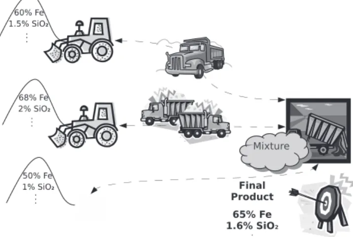
In this problem, the objective is to determine the extraction rate at each pit in a way that production and quality goals are satisfied, and to minimize the number of trucks needed for the production process. The Fig. 1shows a typical production scenario for the problem here described. In this figure, there are equipments as-signed to only two pits. The quantity extracted from each pit de-fines the quality of the final product (ore mixture), since each pit has a known composition.

4. Mathematical model

This section presents a new mixed integer programming (MIP) model based on goal programming (Romero, 2004) to

solve OPMOP. This model refers to production planning for one hour, replicated while there is not any exhausted pit and operational conditions of the mine remain the same. The objec-tive is to minimize the deviations of the production and quality goals and to reduce the number of vehicles required for the operation.

Let the parameters be:

O set of ore pits;

W set of waste rock pits;

F set of ore and waste rock pits, i.e.,F=O[W;

P set of control parameters analyzed in the ore (% Fe, SiO2,

etc.);

S set of shovels;

T set of mining trucks;

Or recommended rate of mining for ore (ton/hour);

Ol minimum rate of mining for ore (ton/hour);

Ou maximum rate of mining for ore (ton/hour);

Wr recommended rate of mining for waste rocks (ton/hour);

Wl minimum rate of mining for waste rocks (ton/hour);

Wu maximum rate of mining for waste rocks (ton/hour);

a

a

b penalty for negative deviation from the production of

waste rocks;

b+ penalty for positive deviation from the production of waste rocks;

pij percentage of the control parameterjin piti(%);

prj recommended percentage for the control parameterj in

the mixture (%);

plj minimum allowable percentage for the control parameterj

in the mixture (%);

puj maximum allowable percentage for the control parameter

jin the mixture (%);

kj penalty for a negative deviation of the control parameterj in the mixture;

kþ_j penalty for a positive deviation of the control parameterj in the mixture;

x

Qui maximum rate of mining for piti(ton/hour);

Txl maximum rate of use for truckl(%);

Slk minimum productivity for shovelk(ton/hour);

Suk maximum productivity for shovelk(ton/hour);

capl capacity of truckl(ton);

ctil total cycle time of trucklin piti(min);

glk 1, if trucklis compatible with shovelk; and 0, otherwise.

Consider also the following variables of decision: xi mining rate of piti(ton/hour);

yik 1, if shovelkoperates in piti; and 0, otherwise.

nil number of trips that trucklperforms to piti;

D

o negative deviation from the recommended ore production (ton/hour);

Dþo positive deviation from the recommended ore production (ton/hour);

D

w negative deviation from the recommended waste rock pro-duction (ton/hour);

Dþw positive deviation from the recommended waste rock pro-duction (ton/hour);

dj negative deviation of the control parameterjin the mix-ture (ton/hour);

dþj positive deviation of the control parameterjin the mixture (ton/hour);

Ul 1, if trucklis being used; and 0, otherwise.

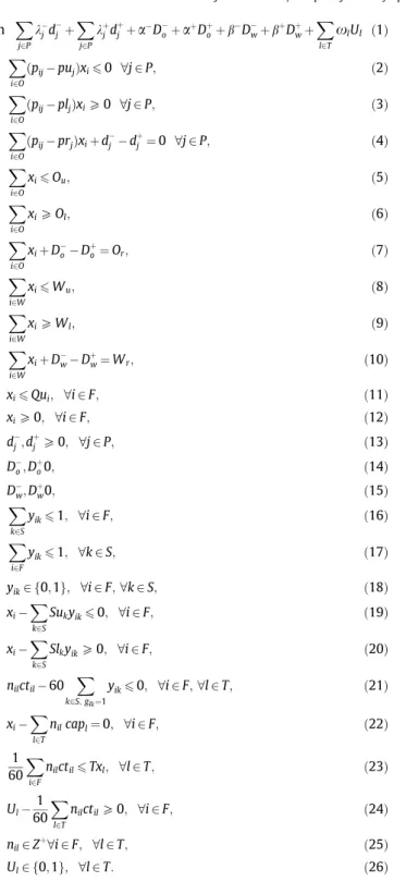
Next, the Eqs.(1)–(26)present the MIP model for the problem in focus.

min X

j2P k

jdj þ X

j2P kþ

jdþj þ

a

a

l2T

x

X

i2O

ðp_ijpu_jÞxi60 8j2P; ð2Þ X

i2O

ðpijpljÞxiP0 8j₂P; ð3Þ

X

i2O

ðpijprjÞxiþdj dþj ¼0 8j2P; ð4Þ X

i2O

xi6Ou; ð5Þ

X

i2O

xiPOl; ð6Þ

X

i2O

xiþDoDþo¼Or; ð7Þ

X

i2W

xi6Wu; ð8Þ

X

i2W

xiPWl; ð9Þ

X

i2W

xiþDwDþw¼Wr; ð10Þ

xi6Qui; 8i2F; ð11Þ

xiP0; 8i2F; ð12Þ

d_j;dþ_j P0; 8j2P; ð13Þ

D

o;Dþo0; ð14Þ

D

w;Dþw0; ð15Þ

X

k2S

yik61; 8i2F; ð16Þ

X

i2F

yik61; 8k2S; ð17Þ

yik2 f0;1g; 8i2F;8k2S; ð18Þ

xi X

k2S

Sukyik60; 8i2F; ð19Þ

xi X

k2S

SlkyikP0; 8i2F; ð20Þ

nilctil60 X

k2S;glk¼1

y_ik60; 8i₂F;8l₂T; ð21Þ

xi X

l2T

nilcapl¼0; 8i2F; ð22Þ

1 60

X

i2F

nilctil6Txl; 8l2T; ð23Þ

Ul1

60

X

l2T

nilctilP0; 8i₂F; ð24Þ

nil2Zþ8i2F; 8l2T; ð25Þ

Ul2 f0;1g; 8l2T: ð26Þ

The objective function (1) seeks to minimize the differences with regard to production goals of ore and waste rock, quality targets of the mixture, as well as to reduce the number of trucks used. The constraints (2)–(15) model the classic problem of blending with goals. Constraints(2) and (3)assure that the max-imum and minmax-imum limits for the control parameters must be verified, respectively. Constraints(4), together with the objective function, aim to meet the recommended percentage for the con-trol parameters. Constraints(5) and (6)guarantee that the maxi-mum and minimaxi-mum production of ore are verified. The constraints (8) and (9) model the same, but considering waste rock. Constraints (7) and (10) relate respectively to the care of the production targets of ore and waste rock, while the con-straints(11)limit the maximum mining rate defined by the user for each pit.

The other constraints which complement the model can be di-vided into two groups. The first concerns the allocation of shovels and productivity range in order to justify the equipment use. The second is related to the allocation of trucks for material transport in the mine.

For the first group, constraints(16)define that at most one sho-vel can be allocated to each pit, while constraints(17)define that each shovel can be allocated to one pit at most. Constraints(18) define that the variablesyik are binary. Each constraint(19) and (20)limits, respectively, the maximum and minimum mining rate defined by shovelkallocated to piti.

In the second group of constraints, each constraint(21)forces the truck to only perform trips where there is compatible shovel allocated. The constraints(22)are such that the mining rate of a pit is equal to the total production of the trucks allocated to that pit. The constraints(23)ensure that each truck lis in operation for at mostTxl% in 1 hour. The constraints(24), together with the

objective function, force the number of trucks used to be penalized. The constraints(25)force the number of trips that a truck performs to a pit to be a positive integer value. Constraints(26)indicate that the variablesUlare binary.

5. Heuristic model

5.1. Representation of a solution

A solution is represented by a matrixR= [YjN], whereYis a ma-trixjF_j 1 andNis a matrixjF_{j j}T_j.

Each cellyiof the matrixYjFj1represents the shovelkallocated

to piti. A value1 means that there is not any shovel allocated to piti. If there are not any trips made to piti, the shovelkassociated to that pit is consideredinactiveand it is not penalized for a pro-duction below the minimum for a shovel.

In the matrixN_jFjjTj, each cellnilrepresents the number of trips

that each truckl₂Tperforms to a piti₂F. A value0(zero) means that there are not any trips allocated to the trucklto the piti, while a value1 indicates that the truck and the shovel allocated to that pit are not compatible.

Fig. 2illustrates a solution involving four trucks, four pits and three shovels. In this figure, for example, the truck 1 makes two trips to pit 1 and one trip to pit 3. The shovel 2 is assigned to pit 4 and the truck 1 is incompatible with it. In this solution, pit 2 is available.

From Y, N and the cycle times from the matrix CT(jF_{j j}T_j dimensional) the extraction rate at each pit is determined, as well as the sum of the cycle times for each truck.

5.2. Neighborhoods

To explore the solution space of the problem, eight movements were developed. Each movement defines a neighborhood N(), which are presented in Sections5.2.1–5.2.8.

5.2.1. Movement number of trips – NNT(s)

This movement increases or decreases the number of trips of trucklto pitiwhere there’s an allocated compatible shovel. Thus, in this movement, a cellnilof the matrixNhas its value increased

or decreased by one trip.

5.2.2. Movement load – NL_(s)

Consists of changing two separate cellsyiandykof the matrixY,

between shovels and trucks, the trips made to that pits are relo-cated along with the shovels.

5.2.3. Movement relocate trip from a truck – NTT_(s)

Consists of choosing two cellsnilandnklfrom the matrixNand

passing one trip fromniltonkl. Thus, in this movement, the truckl

cancels one trip to pitiand does it at another pitk. Compatibility restrictions between equipment are respected in this movement, so the trip relocation is only done when there’s compatibility be-tween them.

5.2.4. Movement relocate trip from a pit – NTP_(s)

Two cellsnilandnikfrom the matrixNare chosen and a unit of

nilis relocated tonik. So this movement consists of relocating one

trip from trucklto truckkwhich are both working at piti. Compat-ibility restrictions between equipment are respected in this move-ment, so the trip relocation is only done when there’s compatibility between them.

5.2.5. Movement pit operation – NPO_(s)

Consists of removing from operation the shovel that is allocated to piti. The movement removes all the trips made to this pit, leav-ing this shovelinactive. The shovel is again put in operation as soon as a new trip is associated to it.

5.2.6. Movement truck operation – NTO_(s)

Consists of selecting a cellnilfrom the matrixNand zero-fill its

content, meaning that the truckldoes not operate in pitianymore.

5.2.7. Movement swap trips – NST_(s)

Two cells of the matrixNare selected and one trip is relocated from one to another. This movement can occur in any cell of the matrix N if compatibility restrictions between equipments are respected.

5.2.8. Movement swap shovels – NSS_(s)

Consists of swapping two separate cellsyiandykfrom the

ma-trixY, i.e. exchanging the shovels that operate in pitsiandk. This movement is similar to the movement Load (Neighborhood NL), because the shovels are also exchanged, but the trips made to these pits are not exchanged. To maintain compatibility between the shovels and trucks, the trips made by incompatible equipment are removed.

Fig. 2shows examples of these movements, wheremis a move-ment that belongs to the neighborhoodN(s). In this figure, a signal * close to a number means the modification made in the solutions. For example, solutionsmTT_{differs ofsin relation to the trips of}

the truck 2 for the pits 1 and 3. This neighbor was obtained froms by reassigning one trip of the truck 2 from the pit 1 to the pit 3. Now, this truck realizes three trips to the pit 1 and one trip to the pit 3.

5.3. Evaluation of a solution

As the developed movement can generate infeasible solutions, a solution is evaluated by a mono-objective function f:S_!R, where Srepresents the set of all possible solutions sgenerated from the movements presented in the previous section. This function f, defined by Eq. (27), to be minimized, consists of two parts: first, the objective function itself (Eq. (1) from the mathematical programming model) and second, a group of func-tions that penalize the occurrence of infeasibility in current solution.

f_ðs_{Þ ¼}fMP ðs_{Þ þ}fp

ðs_{Þ þ}X j2P

fq jðsÞ þ

X

l2T fu

lðsÞ þ

X

k2S fc

kðsÞ: ð27Þ

In Eq.(27),fMP_{(s) is the objective function from the}

mathemat-ical programming model given by Eq.(1), i.e.fMP_{(s) evaluatess}

2S considering production and quality goals, as well as the number of trucks used; fp(s) evaluates s considering unmet production goals for ore and waste rock; fq

infeasibility of thejth control parameter;fu

lðsÞevaluatess

regard-ing disrespect of the maximum use rate of thelth truck; andfc kðsÞ

evaluatessfor disrespect of the productivity limits of the shovel k.

5.4. Initial solution generation

An initial solution to the problem is built in two steps. First, the allocation of the shovels and the distribution of trips are done for the waste rock pits; secondly, for the ore pits. This strategy is adopted because in the waste rock pits it is important to meet pro-duction and not necessary to observe the quality of the control parameters.

In the first step a greedy heuristic is used (Algorithm 1). In this algorithm, we define the ‘‘best” choice according to our greedy criterion as follows: for waste rock pits, the best is the one with the greatest mass; for shovels, the best is the one with the greatest production and for trucks, the largest one is the best.

Algorithm 1. BuildWasteSolution

Input:S,T,W,Wr

Output: SolutionsW

T Set of available trucks ordered by their capacities (the first is the truck that has the greatest capacity); S Set of available shovels ordered by their maximum

productivities (the first is the shovel that has the greatest productivity);

W Set of available waste rock pits ordered according to their maximum rates of mining (the first is the pit that has the greatest rate);

whilethe waste rock production is less than the recommended oneandthere are available waste rock pitsdo

Select the first pitifromW;

ifthere is no shovel at pit ithen

ifAll shovels are assignedthenRemove pitifromWelse

UpdatesWassigning the best available shovel to piti;

end

if Pit i was not removed from W then

Find a truckl₂Tsuch that: (a) it is compatible with the shovel assigned to piti; (b) it can do one more trip; (c) its capacity does not violate the shovel’s maximum

production;

iftruck l existsthenUpdatesWassigning the maximum

number of trips of thel-truck to piti;

else Remove pitifromW;

end end returnsW;

For the second step, a heuristic based onGRASP_{is used. In its}

original form (Feo and Resende, 1995),GRASP_{is an iterative}

meth-od that has two phases: construction and local search. The con-struction phase builds a feasible solution, whose neighborhood is explored by local search. The best solution over allGRASPmax iter-ations is returned as the result.

For the ore pits, the classification of the candidate elements to be inserted in the solution is made considering that: (a) the best pit is the one that has the least deviation of the control parameter levels in relation to the targets; (b) the best shovel is the one that provides the greatest production and (c) the best truck is the one that has the smallest capacity.

In order to select the ore pits in the second step, a guide function g, which measures the deviation values of the quality goals, is used. According to this function, it is more likely to choose the ore pit that best helps to minimize the deviations from the quality targets. First, all candidate pits (CL) are sorted with respect to the functiong, where CL is the set of available pits. FromCL, the construction phase creates a restricted candi-date list (RCL) using the best qualified ore pits according to the guide function. The parameter

c

c

Afterwards, the procedure chooses a pit randomly from this list using a strategy proposed byBresina (1996), and adds it to the partial solution. The strategy consists in assigning a rank-based probability for each candidate pit inRCL. The bias function bias(r) = 1/(r) is associated to therth best classified pit. Then, each candidate pit is chosen with probability p_ðr_{Þ ¼}bias_ðr_Þ=

P

i¼1;...;jRCLjbiasðiÞ. The construction phase ends when the ore

pro-duction goal is reached or when there are no more pits or shovels available. In each iteration of this construction, the shovel with the greatest production and the truck that has the smallest capac-ity is chosen. Algorithm 2 outlines the second step of the con-struction phase.

According toLourenço et al. (2003), the initial solution is cer-tainly important to achieve high quality solutions in the first in-stants of the search. Since the construction phase of GRASP _is

often able to produce solutions close to some local optimum ( Re-sende and Ribeiro, 2010) and our local search procedures are very expensive (Section5.2), we opted for executing a number of itera-tions of the construction procedure alone before proceeding do the next phase.

Algorithm 2. BuildOreSolution

Input:sW,

c

Output: Solutions0 s0 sW;

T Set of available trucks ordered by their capacities (the first is the truck that has the smallest capacity); S Set of available shovels ordered by their maximum

productivities (the first is the shovel that has the greatest productivity);

while the ore production is less than the recommended oneand

there are available ore pitsdo

CL Set of available ore pitsi2Oordered according to functiong;

jRCL_j=d

c

Selecti2RCLaccording to the bias function;

if there is no shovel at pit ithen

if All shovels are assignedthenRemove pitifromCLelse

Updates0assigning the best available shovel to piti;

end

ifPit i was not removed from CL then

Find a truckl₂Tsuch that: (a) it is compatible with the shovel assigned to piti; (b) it can do one more trip; (c) its capacity does not violate the shovel’s maximum production;

if truck l existsthenUpdates0assigning onel-truck trip

for the piti;

elseRemove pitifromCL;

5.5. Proposed algorithm

The proposed algorithm, called GGVNS_{, combines ideas from} GRASP_{(Resende and Ribeiro, 2010) and}General Variable Neighbor-hood Search–GVNS_{(Hansen et al., 2008b) procedures. Algorithm 3}

outlines the steps.

Algorithm 3.GGVNS

Input: setsO,W,P,S,T,. . .(see parameters in Section4)

Input:

c

Output: Solutions

1 sW BuildWasteSolution()

2 s0 best solution fromGRASPmaxcalls to BuildOreSolution(sW,

c

3 s VND(s0)

4 p 0

5 while stop criterion not satisfieddo

6 iter 0

7 whileiter<IterMaxandstop criterion not satisfieddo

8 s0 _s

9 fori= 1top+ 2do

10 k SelectNeighborhood() 11 s0 _Shake(s0_,k)

12 end

13 s00 _VND(s0₎ 14 iff(s00_{) <f(s)then}

15 s s00

16 p 0

17 iter 0

18 end

19 iter iter+ 1

20 end

21 p p+ 1

22 end

23 returns

Building an initial solutions0(lines 1 and 2 of Algorithm 3) is

made by the procedure described in subsection 5.4. The local search (lines 3 and 13 of Algorithm 3), in turn, uses theVND

proce-dure (see the pseudo-code in Algorithm 3) with the movements described in Section5.2.

Whenever a given number of iterations without improvement is reached, theGGVNSalgorithm appliesp+ 2 times theShake proce-dure, using a previously selected neighborhood. The procedure SelectNeighborhood(line 10 of the Algorithm 3) works as follows. We randomly select a neighborhoodkfrom the list {NSS_,NTO_,NPO_,

NST, NNT, NL} with probabilities {10%, 10%, 10%, 20%, 30%, 20%}, respectively. We observed that some neighborhoods are more likely to contain solutions which are significantly different of the current solution. These probabilities reflect this observation. Each Shake(s0_{,k) call (line 11 of Algorithm 3) performs a random}

move-ment from neighborhoodkof the shaken solutions0_{. AfterIterMax}

iterations without improvement, we incrementpin order to gener-ate solutions which become increasingly distant from the current location in the search space.

The local search applied on the solution returned by theShake procedure is based on theVND _{procedure (line 13 of Algorithm}

3). IfVND_{finds a better solution, the variable}preturns to the low-est value, that is,p= 0.

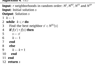
Algorithm 4.VND

Input:rneighborhoods in random order:NL,NNT,NTTandNTP

Input: Initial solutions

Output: Solutions

1 k 1

2 while k6rdo

3 Find the best neighbors0_2N(k)_(s)

4 iff(s0_{) <f(s)then}

5 s s0

6 k 1

7 end

8 else

9 k k+ 1

10 end

11 end

12 returns

As in the preliminary tests some neighborhoods did not produce good quality solutions or spent too much processing time to achieve a good one, only a small group of neighborhoods was used in the local search. Thus, the VND _{used the following}

neighbor-hoods:NL_,NNT_,NTT_andNTP_{. Furthermore, theVNDprocedure (see}

Algorithm 4) operates in the neighborhoods in a random order, which can be different at each VND _{call (more details in the}

Section7).

6. Scenarios description

The scenarios utilized for the tests refer to an iron mining com-pany located in the state of Minas Gerais, Brazil and are available at http://www.iceb.ufop.br/decom/prof/marcone/projects/mining.html. Table 1describes some characteristics of the instances. The col-umns ‘‘# pits, # shovels, # trucks and par.” indicate the number of pits, shovels, trucks and control parameters (chemical and/or gran-ulometric), respectively. The column ‘‘characteristics” shows the number and the truck capacity or the shovel productivity. For example, the pair (15, 50t) means there are 15 trucks (or shovels) of 50 ton of capacity (or maximum productivity).

The following weights were adopted in the evaluation function:

a

_a

j ¼kþj ¼18j2T;

x

75%₈l2V.

7. Computational experiments and analysis

The proposed algorithm, so-calledGGVNS_{, was coded in C++}

programming language and compiled with the GNU Compiler Col-lection version 4.0. The mathematical programming model was written in AMPL language (Fourer et al., 1990) and solved by the

ILOG CPLEXoptimizer version 11.01 (ILOG, 2008), using default

parameters. Both heuristic and exact models were tested in a PC Pentium Core 2 Quad (Q6600), 2.4 GHz, with 8 GB of RAM, running Windows Vista.

All the experiments considered the following parameters: Iter-Max= 5000,GRASPmax= 10,000 and

c

As mentioned inHansen et al. (2008b), one important decision to build an efficientVND_{procedure is to select an application order}

of the different neighborhoods. In a preliminary set of experiments (10 runs for each instance) we tried to discover the optimal se-quence of neighborhood application, that is, the one which, in aver-age, produces better solutions in a limited amount of time when running the GGVNS_{algorithm. To accomplish this objective, we}

considering each one of the neighborhoods as the first neighbor-hood in the sequence, and the remaining ones were chosen in a random order, at eachVND_{call (Phase I columns of theTable 2).}

For simplicity, the neighborhoodsNL_,NNT_,NTT_,NTP_{are denoted by}

L,NT,TT,TP, respectively, in theTable 2. Considering these results, we observed better results in relation to the average gap (the last row in theTable 2) when selectingNL_{as the first neighborhood.}

Therefore, this neighborhood was kept as the first in the sequence. After that, we ran experiments to define the second neighbor-hood of the sequence. From the remaining neighborneighbor-hoods {NNT_,

NTT_{, N}TP_},NTT _{produced the best results in relation to the same}

metric used previously (Phase II columns inTable 2), being se-lected to occupy the second position.

Finally, additional experiments (Phase III columns inTable 2) indicated that it would be better to search in the neighborhood NTP_{before proceeding to search inN}NT_{. In these experiments, we}

observed that our ‘‘best” sequence of neighborhoods does not out-perform many of the results produced when the neighborhood application order was partially random (Columns 2–8 inTable 2). This motivated us to perform an additional experiment in which

the neighborhood application sequence was completely random at eachVND_{call. This experiment produced the best results,}

indi-cating that the random selection of neighborhoods to search is the best option (Random column in theTable 2). The results in Ta-ble 3were produced using this last strategy.

In the first set of experiments we evaluatedGGVNS_considering

its ability to produce good solutions in a short amount of time. Considering the needs of decision makers, we limited the execu-tion time to 2 minutes, which is a typical value for the maximum tolerance in a real case. TheGGVNS_{algorithm was applied 30 times}

for each instance. ForCPLEX_{, we also allowed longer execution}

times for searching for the optimal solution.

Results of this set of experiments appear inTable 3. In this table, column ‘‘best known” refers to the best known cost found in all our experiments. In column ‘‘opt.” we indicate by ‘‘p” instances in which CPLEX _{succeeded in proving the optimality of the best}

known cost. Columns ‘‘gap” are computed as follows: consider that f

i is the best known cost for instancei(optimal cost for some

in-stances),fCPLEX

i is the upper bound obtained at the end ofCPLEX

execution for instanceiandfGGVNS

i is the average value found in Table 1

Characteristics of the instances.

Inst. # Pits Shovels # par. Trucks

# Shovels Characteristics # Trucks Characteristics

opm1 17 8 (4, 900t), (2, 1000t) 10 30 (15, 50t), (15, 80t)

(2, 1100t)

opm2 17 8 (4, 900t), (2, 1000t) 10 30 (15, 50t), (15, 80t)

(2, 1100t)

opm3 32 7 (2, 400t), (2, 500t) 10 30 (30, 50t)

(1, 600t), (1, 800t) (1, 900t)

opm4 32 7 (2, 400t), (2, 500t) 10 30 (30, 50t)

(1, 600t), (1, 800t) (1, 900t)

opm5 17 8 (4, 900t), (2, 1000t) 5 30 (15, 50t), (15, 80t)

(2, 1100t)

opm6 17 8 (4, 900t), (2, 1000t) 5 30 (15, 50t), (15, 80t)

(2, 1100t)

opm7 32 7 (2, 400t), (2, 500t) 5 30 (30, 50t)

(1, 600t), (1, 800t) (1, 900t)

opm8 32 7 (2, 400t), (2, 500t) 5 30 (30, 50t)

(1, 600t), (1, 800t) (1, 900t)

Table 2

Results of the preliminary experiments.

Instance Phase I Phase II Phase III Random

L NT TT TP LNT LTT LTP LTTNTTP LTTTPNT

opm1 232.80 1,816.40 235.54 236.85 232.66 232.36 233.11 1696.35 236.20 230.12 opm2 335.37 340.70 2686.72 326.78 350.27 340.93 327.30 332.68 338.18 256.56 opm3 164,058.99 164,054.62 164,057.97 164,067.40 164,059.08 164,057.56 164,054.60 164,057.96 164,054.29 164,064.68 opm4 164,138.64 164,143.77 164,126.98 164,123.92 164,118.64 164,158.45 164,123.00 164,135.01 164,133.37 164,153.92 opm5 229.86 1692.72 1690.83 229.07 232.01 229.58 228.93 450.71 231.05 228.09 opm6 326.60 330.51 308.14 2703.00 319.09 325.50 2,672.08 308.21 312.88 237.97 opm7 164,021.50 164,021.65 164,021.67 164,021.58 164,021.55 164,021.86 164,021.59 164,021.56 164,021.66 164,021.89 opm8 164,024.32 164,024.36 164,024.53 164,023.89 164,023.90 164,023.58 164,024.43 164,024.08 164,023.62 164,027.29

GAP (%)

opm1 2.501 699.753 3.707 4.284 2.440 2.309 2.639 646.894 3.996 1.321

opm2 30.814 32.894 947.986 27.465 36.628 32.985 27.669 29.766 31.913 0.074

opm3 0.019 0.017 0.019 0.025 0.019 0.019 0.017 0.019 0.017 0.023

opm4 0.050 0.053 0.043 0.041 0.038 0.062 0.040 0.048 0.047 0.059

opm5 1.240 645.560 644.726 0.892 2.189 1.120 0.834 98.516 1.768 0.462

opm6 38.052 39.702 30.247 1042.531 34.876 37.586 1,029.463 30.278 32.251 0.588

opm7 0.002 0.003 0.003 0.003 0.002 0.003 0.003 0.003 0.003 0.003

opm8 0.003 0.003 0.004 0.003 0.003 0.003 0.004 0.003 0.003 0.005

the 30 executions ofGGVNS_{algorithm, gap is computed for each}

in-stanceifor theCPLEX_optimizerðgapCPLEX

i Þand forGGVNSðgap

GGVNS

i Þ

in Eqs.(28) and (29), respectively.

gapCPLEX

i ¼

fCPLEX i fi

f i

; ð28_Þ

gapGGVNS

i ¼

_fGGVNS i fi

f i

: ð29_Þ

As can be seen inTable 3, considering the time limit of two min-utes, CPLEX was able to prove the optimality of the solution only in two of the eight instances. In addition, for another two instances (opm2 and opm5), CPLEX presented very high gap. For the other hand,GGVNS_{presented near best known solutions (gap < 1.5%) in}

all instances, even with the time limit constraint. A remarkable re-sult forGGVNS_{appeared in the hard instances opm2 and opm5. In}

these instances, CPLEX could not provide a solution satisfying pro-duction goals within 2 minutes, while GGVNS _{always produced}

solutions satisfying this requirement in the restricted time. In in-stances 3, 4, 7 and 8 the solutions presented a very high cost. We observed that this happens due to a waste production goal which cannot be satisfied, generating a constant in the objective function. We decided to not change this goal to maintain compatibility with previous works.

One important result would be the discovery of the optimal solution for the remaining instances 1–6. This motivated us to per-form the longer runs (two hours) of the CPLEX optimizer. Within this time limit, CPLEX found the optimal solution for two addi-tional instances: opm3 and opm4. InFigs. 3–5we plotted the evo-lution of the lower and upper bounds during CPLEX search for

some instances. As can be seen, although CPLEX heuristics man-aged to improve the upper bounds, the lower bounds remained stable. After a certain amount of time, both lower and upper bounds stagnated, which led us to believe that longer execution times would not suffice to produce optimal solutions using our formulation.

Below we analyze the results of the proposed algorithm with re-gard to the quality of the control parameters. For each instance, considering the 30 executions ofGGVNS_{, we calculated the largest}

Table 3

Experimental results: mathematical programming model in CPLEX andGGVNSheuristic.

Instance Best known CPLEX GGVNS

2 hours 2 minutes

Cost Opt.a _{Cost Gap Cost Gap Best Average Std. dev. Gap}

opm1 227.12 227.12 0.00 230.65 1.55 230.12 230.12 0.01 1.32

opm2 256.37 257.66 0.50 4858.39 >100.00 256.37 256.56 0.26 0.07

opm3 164,027.15 p 164,027.15 0.00 164,042.60 0.01 164,039.12 164,064.68 17.24 0.02 opm4 164,056.68 p 164,056.68 0.00 164,061.80 0.00 164,099.66 164,153.92 29.43 0.06

opm5 227.04 227.04 0.00 7229.07 >100.00 228.09 228.09 0.00 0.91

opm6 236.58 236.58 0.00 236.58 0.00 236.58 237.97 2.38 0.59

opm7 164,017.46 p 164,017.46 0.00 164,017.46 0.00 164,021.38 164,021.89 0.34 0.00 opm8 164,018.65 p 164,018.65 0.00 164,018.65 0.00 164,023.73 164,027.29 1.60 0.00

a _{Considering CPLEX mipgap tolerance610}5_{, except for opm3, which used mipgap tolerance610}4_.

Fig. 3.Evolution of upper and lower bounds in CPLEX – instance opm1.

Fig. 4.Evolution of upper and lower bounds in CPLEX – instance opm2.

absolute error between the recommended percentageprjfor the

control parameterjin the blending and the encountered percent-ageepjifor this control parameter in all executionsiof theGGVNS.

For this calculation we chose the solution of theith execution of theGGVNS_{in which the percentage}epjiis the farthest from the

rec-ommended percentageprj. The symbol + in theFigs. 6 and 7

repre-sents the biggest absolute error for the instances opm2 and opm3, respectively. We also calculated the absolute error between the recommended percentageprj for the control parameterjin the

blending and the average of the encountered percentagesepj for

this control parameter in theGGVNS_{solutions. The symbolh in}

theFigs. 6 and 7represents this error for the instances opm2 and opm3, respectively.

While the absolute errors for the instance opm2 (Fig. 6) vary from 0.32% up to 11.49%, they reach 40.53% in the instance opm3 (Fig. 7). This is because the minimum and maximum allowable percentages for the control parameters in the mixture vary from one instance to another. In the instance opm3 these values are, respectively, 0% and 100%, that is, the percentage of each control parameter can vary from 0% to 100% in the solution. On the other hand, in the instance opm2, the difference between the minimum and maximum allowable percentages is smaller, so forcing the encountered percentages for the control parameters to be closer to the recommended percentages. For the remaining instances, the error behavior is similar to the one obtained for opm2 or opm3.

8. Conclusions

This work dealt with the operational planning of mines consid-ering the dynamic allocation of trucks. Because of the complexity of this combinatorial problem, we proposed a hybrid heuristic algorithm, calledGGVNS_{, which combines the heuristic procedures} GRASP_{and General Variable Neighborhood Search to solve it.}

Using instances from literature, the proposed heuristic algo-rithm was compared to the optimizer CPLEX 11.0.1 applied to a mathematical programming model, also developed in this work. It was found that theGGVNS_{algorithm is competitive with CPLEX}

solver, sinceGGVNS_{is able to find good quality solutions quickly}

with low variability. Since staff decisions have to be made quickly, the results validate the use of the proposed algorithm as a tool for decision support.

As future works we consider to integrate the mathematical pro-gramming solver withGGVNS_{, with the aim of combining the fast}

solution times ofGGVNS _{with the systematic exploration of the}

search tree of exact solvers. We are also studying the improvement ofGGVNS_{by adding a Path Relinking strategy to work with an elite}

pool of solutions.

Acknowledgements

The authors acknowledge FAPEMIG (Grants CEX 2991-06.1/07, CEX 357-09 and CEX 01201-09) and CNPq (Grant 474831/2007-8) for supporting the development of this research. We also thank the anonymous referees for their constructive comments, leading to an improved version of this paper.

References

Alvarenga, G.B., 1997. Optimal Dispatch of Trucks in an Iron Mine Using Genetic Algorithms with Parallel Processing (in Portuguese). Master’s Thesis, Programa de Pós-Graduação em Engenharia Elétrica, Escola de Engenharia, UFMG, Belo Horizonte, Minas Gerais, Brazil.

Boland, N., Dumitrescu, I., Froyland, G., Gleixner, A.M., 2009. LP-based disaggregation approaches to solving the open pit mining production scheduling problem with block processing selectivity. Computers and Operations Research 36, 1064–1089.

Bresina, J.L., 1996. Heuristic-biased stochastic sampling. In: Proceedings of the 13th National Conference on Artificial Intelligence. AAAI Press, Portland, pp. 271– 278.

Chanda, E.K.C., Dagdelen, K., 1995. Optimal blending of mine production using goal programming and interactive graphics systems. International Journal of Surface Mining, Reclamation and Environment 9, 203–208.

Ezawa, L., Silva, K.S., 1995. Dynamic allocation of trucks aiming quality (in Portuguese). In: Proceedings of the VI Congresso Brasileiro de Mineração. Salvador, Bahia, Brazil, pp. 15–19.

Feo, T.A., Resende, M.G.C., 1995. Greedy randomized adaptive search procedures. Journal of Global Optimization 6, 109–133.

Fourer, R., Gay, D.M., Kernighan, B.W., 1990. A modeling language for mathematical programming. Management Science 36 (5), 519–554.

Glover, F., Kochenberger, G. (Eds.), 2003. Handbook of Metaheuristics. Kluwer Academic Publishers.

Godoy, M., Dimitrakopoulos, R., 2004. Managing risk and waste mining in long-term production scheduling of open-pit mines. SME Transactions 316, 43–50. Guimaraes, I.F., Pantuza, G., Souza, M.J.F., 2007. A computational simulation model

to validate results by dynamic allocation of trucks in open-pit mines (in Portuguese). In: Proceedings of the XIV Simpósio de Engenharia de Produção (SIMPEP), Bauru, São Paulo, Brazil, 11p.

Hansen, P., Mladenovic, N., 2001. Variable neighborhood search: principles and applications. European Journal of Operational Research 130, 449–467. Hansen, P., Mladenovic, N., Pérez, J.A.M., 2008a. Variable neighborhood search.

European Journal of Operational Research 191, 593–595.

Hansen, P., Mladenovic, N., Pérez, J.A.M., 2008b. Variable neighborhood search: methods and applications. 4OR: Quarterly Journal of the Belgian, French and Italian Operations Research Societies 6, 319–360.

ILOG, 2008. CPLEX 11.0 User’s Manual.

Lourenço, H.R., Martin, O.C., Stützle, T., 2003. Iterated local search. In: Glover, F., Kochenberger, G. (Eds.), Handbook of Metaheuristics. Kluwer Academic Publishers, Boston.

Merschmann, L.H.C., 2002. Development of an optimization and simulation system for the analysis of production scenarios in open-pit mines (in Portuguese). Master’s Thesis, Programa de Engenharia de Produção/COPPE, UFRJ, Rio de Janeiro, Brazil.

Fig. 6.Deviation of the control parameters in the mixture for the instance opm2.

Mladenovic, N., Hansen, P., 1997. A variable neighborhood search. Computers and Operations Research 24, 1097–1100.

Papadimitriou, C.H., Steiglitz, K., 1998. Combinatorial Optimization: Algorithms and Complexity. Dover Publications, Inc., New York.

Resende, M.G.C., Ribeiro, C.C., in press. Grasp. In: Burke, E.K., Kendall, G. (Eds.), Search Methodologies, second ed. Springer. Available at:<http://www.ic.uff.br/ celso/artigos/grasp.pdf>.

Romero, C., 2004. A general structure of achievement function for a goal programming model. European Journal of Operational Research 153, 675–686.

Sgurev, V., Vassilev, V., Dokev, N., Genova, K., Drangajov, S., Korsemov, C., Atanassov, A., 1989. Trasy – an automated system for real-time control of the industrial truck haulage in open-pit mines. European Journal of Operational Research 43, 44–52.

White, J.W., Olson, J.P., 1986. Computer-based dispatching in mines with concurrent operating objectives. Mining Engineering 38 (11), 1045–1054.