www.the-cryosphere.net/7/1603/2013/ doi:10.5194/tc-7-1603-2013
© Author(s) 2013. CC Attribution 3.0 License.
The Cryosphere
Decadal changes from a multi-temporal glacier inventory of
Svalbard
C. Nuth1, J. Kohler2, M. König2, A. von Deschwanden2, J. O. Hagen1, A. Kääb1, G. Moholdt1,3, and R. Pettersson4 1Dept. of Geosciences, University of Oslo, Oslo Norway
2Norwegian Polar Institute, Tromsø, Norway
3Institute of Geophysics and Planetary Physics, Scripps Institution of Oceanography, La Jolla, California, USA 4Department of Earth Sciences, Uppsala University, Uppsala, Sweden
Correspondence to:C. Nuth ([email protected])
Received: 17 April 2013 – Published in The Cryosphere Discuss.: 10 June 2013
Revised: 6 September 2013 – Accepted: 10 September 2013 – Published: 18 October 2013
Abstract.We present a multi-temporal digital inventory of
Svalbard glaciers with the most recent from the late 2000s containing 33 775 km2of glaciers covering 57 % of the total
land area of the archipelago. At present, 68 % of the glacier-ized area of Svalbard drains through tidewater glaciers that have a total terminus width of ∼740 km. The glacierized
area over the entire archipelago has decreased by an aver-age of 80 km2a−1 over the past∼30 yr, representing a
re-duction of 7 %. For a sample of∼400 glaciers (10 000 km2)
in the south and west of Spitsbergen, three digital inventories are available from the 1930/60s, 1990 and 2007 from which we calculate average changes during 2 epochs. In the more recent epoch, the terminus retreat was larger than in the ear-lier epoch, while area shrinkage was smaller. The contrasting pattern may be explained by the decreased lateral wastage of the glacier tongues. Retreat rates for individual glaciers show a mix of accelerating and decelerating trends, reflecting the large spatial variability of glacier types and climatic/dynamic response times in Svalbard. Lastly, retreat rates estimated by dividing glacier area changes by the tongue width are larger than centerline retreat due to a more encompassing frontal change estimate with inclusion of lateral area loss.
1 Introduction
Glacier inventories are important for studying the global frozen freshwater resource, and provide a basic dataset for further glaciological, remote sensing and modeling studies. The World Glacier Inventory (WGI), the first global glacier
catalogue, was compiled with classification schemes based on hydrological drainage basins (Müller et al., 1977). WGI contains auxiliary information such as topographic parame-ters, length and volume estimates, and glacier characteriza-tion codes, but it does not include the digitized coordinates of the glacier outlines (WGMS, 1989). Recently, the Global Land Ice Measurements from Space (GLIMS) initiative has provided a scheme for generating a global glacier inventory that retains the raw glacier outline information (Raup et al., 2007). There are some inherent differences between GLIMS and WGI in their structure, application and information they provide (Cogley, 2009), but regional glacier inventories can be relatively easily submitted and linked to both datasets (e.g. Paul et al., 2009; Bolch et al., 2010; Svoboda and Paul, 2010). Moreover, the increasing ease of generating glacier inventories semi-automatically from satellite imagery (Paul et al., 2013) combined with the more frequent coverage of planned satellite missions (e.g. Sentinel-2) facilitate such in-vestigations of multi-temporal glacier inventory changes.
The Arctic archipelago of Svalbard in the North Atlantic is∼57 % glacierized and contains a mix of cirque and
of the Arctic, a period sometimes referred to as the Early 20th Century Warming (Wood and Overland, 2010). Follow-ing a colder period from the 1940s to the 1960s, summer temperatures on Svalbard have been increasing. For the pe-riod 1989–2011, summer temperatures have been increasing at rates of more than 0.5◦C decade−1 at the two long-term
meteorological stations (Førland et al., 2011). This has led to increased glacier volume loss, particularly in western Sval-bard (e.g. Kohler et al., 2007; James et al., 2012).
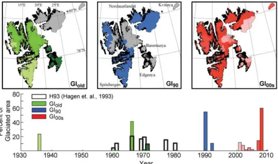
In this study, we present glacier extent snapshots and change rates from the 1930s to 2010 based on 3 digital glacier inventories: GIold, GI90 and GI00s. The inventories
are a key component of a new digital glacier database (König et al., 2013) that is structured after theGlacier Atlas of Sval-bard and Jan Mayen(Hagen et al., 1993), the first complete glacier inventory of the archipelago (referred to as H93 in the rest of this text). GIold and GI90 are derived from two
Norwegian Polar Institute map products; the first is a mixed product of the years 1936, 1960, 1961, 1966, 1969, 1970, and 1971, and the second is from 1990. GI00supdates the
previ-ous inventories using satellite imagery from the years 2000– 2010. We describe the present glaciation of the archipelago through topographic and glaciologic inventory parameters. Furthermore, we discuss the generation and applicability of three glacier inventory change parameters as derived for two epochs: (1) area changes, (2) length changes as estimated by two methods, and (3) glacier tongue width change.
2 Data
2.1 Historic data
Accurate topographic mapping of Svalbard began in the 1950s, when the Norwegian Polar Institute (NPI) under-took to construct maps using analogue photogrammetry of oblique aerial photographs taken in 1936 and 1938. These early maps covered southern and western Spitsbergen, about 22 % of the archipelago. From the late 1950s to the early 1970s, a number of aerial campaigns acquired vertical pho-tographs covering ∼50 % of the archipelago, with major
campaigns in 1966 for northern Spitsbergen and in 1971 for Edgeøya/Barentsøya. Taken together, these maps formed the original S100 (1:100 000) topographic map series published
and distributed by NPI as paper maps. The original S100 map series was digitized by NPI in the 1990s, and forms the basis for GIold.
H93, the original glacier inventory of Svalbard (Hagen et al., 1993), followed the identification and parameter defini-tions outlined by WGMS (1989). It was based upon the S100 paper maps (before digital transformation) but with the old-est data (1936 and 1938) updated using pre-1980 aerial and Landsat imagery. Front positions and areas of H93 were mea-sured from these updated paper maps using a planimeter. The inventory consists of basic data such as glacier name, area,
length, and photo year in table format, but the raw outline locations are not preserved and thus not available digitally in a GIS (geographic information system). For consistency, we preserve the same structure for our new digital glacier inven-tory.
A second major mapping campaign was conducted by NPI in 1990 to acquire vertical aerial photographs over nearly the entire archipelago. In the 1990s and 2000s, NPI created topographic and thematic maps for about 60–70 % of the archipelago using digital photogrammetric techniques and manual feature delineation, which forms the basis for GI90.
There are two exceptions in this updated dataset: the south coast of Austfonna front position was mapped by helicopter with GPS in 1992 (T. Eiken, personal communication, 2013), and a small inland strip within southern Spitsbergen was cov-ered with 1961 and 1970 images (H. Faste Aas, personal communication, 2013). The spatial and temporal coverage of all glacier inventories can be seen in Fig. 1.
2.2 Satellite imagery
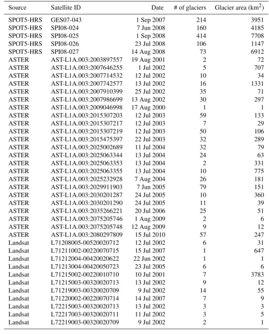
Summer satellite imagery spanning the period 2000–2010 is used as the basis for our third glacier dataset, GI00s
(Ta-ble 1). We prioritize data from sensors that obtain stereo op-tical imagery for creation of orthophotos that are temporally and spatially consistent with the digital elevation models (DEMs) used to generate them. Accordingly, the main data are the DEMs and orthophotos from the SPOT5-HRS (high-resolution sensor) satellite, generated by the IPY project SPIRIT (SPOT 5 stereoscopic survey of Polar Ice: Refer-ence Images and Topographies) (Korona et al., 2009). The SPOT5-HRS collects 5 m panchromatic stereo images that are stereoscopically processed into 40 m DEMs, which are then used for generating orthophotos of the original images. Five SPIRIT acquisitions from 2007 to 2008 cover 71 % of the glacierized area of Svalbard.
The second main satellite data source is the ASTER L1B product, in the form of automatically generated DEMs and orthophotos (AST14DMO, 2010). These have a smaller swath width (60 km) than SPOT5, such that 23 scenes are needed to cover∼16 % of the glacier area. Cloud-free scenes
were not available for 2007–2008, and therefore data from as early as 2000 were required to complete coverage of the archipelago. For the remaining 14 % of the glacier area, no suitable SPOT5-HRS or ASTER scenes were available. For these glaciers, 11 orthorectified Landsat scenes from 2001 to 2007 are used. An additional 17 Landsat and 13 ASTER scenes are used to aid decisions related to perennial snow patches and to delineate glacier margins in areas with sea-sonal snow cover or shade.
2.3 Satellite DEMs
Fig. 1.Spatial and temporal coverage of glacier inventories (GI). The three maps (top) and the filled bars (bottom) show digitally available outlines. The black unfilled bars are the H93 tabular inventory (Hagen et al., 1993). The satellite-based inventory, GI00s(in red), is the first digital inventory covering the entire archipelago. The shades of individual colors in the maps represent time within each inventory. Lighter shades are earlier; i.e. the lightest green is from 1936 and the lightest red from 2001. Grey represents no data.
attributes to the glaciers (Frey and Paul, 2012). The GDEM is a global compilation of stacked and filtered ASTER DEMs (Fujisada et al., 2012) that temporally overlaps GI00s. GDEM
is chosen over other DEMs (SPOT/ASTER) for its consis-tency as a single product covering the entire archipelago. Glacier surfaces in the GDEM have a bumpy texture, a re-sult of the merging of temporally different DEMs of varying quality, especially on the low visual contrast upper glacier areas. Therefore, a low-pass Fourier filter is applied over glacier surfaces to remove the high-frequency noise and min-imize the size of the blunders that occur at the highest eleva-tions (see Appendix A). The filtering reduced standard de-viations of elevation differences with respect to ICESat and SPOT-SPIRIT DEMs and improved visual appearance of the GDEM without changing the overall structure of the surface. Moreover, visual comparisons between the GDEM-derived hydrological basins and those derived from the NPI topo-graphic maps/DEMs, the SPOT-SPIRIT DEMs and individ-ual AST14DMO (2010) DEMs reveal small variations which verify the use of the GDEM for this purpose and infer that rough DEM quality does not have a large impact on drainage basin generation. The largest discrepancies (blunders) oc-cur on the flattest upper regions of ice cap and ice fields where small elevation inconsistencies can sometimes lead to large differences in the determination of a hydrological di-vide. These blunders are manually adjusted to the drainage basins derived from the other DEMs. For the Austfonna ice cap, where the GDEM contains several holes, we use an inde-pendently created DEM (Moholdt and Kääb, 2012), as well as velocity fields derived from SAR interferograms (Strozzi
et al., 2008; Dowdeswell et al., 2008) to delineate ice divides and glacier basins and to generate topographic parameters.
3 Methods
3.1 Georeferencing
The various DEMs and orthoimages must be correctly geo-referenced for merging into a common dataset. While the SPOT5 and ASTER orthoimages are internally consistent with the associated DEMs, the geolocation accuracy is de-pendent upon the accuracy of the satellite position determina-tion (orbital parameters) and instrument pointing (auxillery attitude information), and thus the relative DEM/orthophoto may not necessarily be located precisely on the ground. We co-register the DEMs to ICESat laser altimetry data (Zwally et al., 2012) over non-glacier topography (Nuth and Kääb, 2011) and apply the horizontal component of the correction vector to the orthoimages. We reference ICESat rather than the NPI S100 map series because ICESat data are acquired in a consistent way over the entire archipelago, while S100 is a merged product originating from various sources (ana-logue and digital photogrammetry) and dates (1960s–1990s). The horizontal consistency of ICESat to the 1990 DEM is
≈ ±3 m (Nuth and Kääb, 2011). For the LANDSAT scenes,
Table 1.Data sources used for the compilation of the most recent Svalbard glacier inventory, GI00s.
Source Satellite ID Date # of glaciers Glacier area (km2)
SPOT5-HRS GES07-043 1 Sep 2007 214 3951
SPOT5-HRS SPI08-024 7 Jun 2008 160 4185
SPOT5-HRS SPI08-025 1 Sep 2008 414 7708
SPOT5-HRS SPI08-026 23 Jul 2008 106 1147
SPOT5-HRS SPI08-027 14 Aug 2008 73 6912
ASTER AST-L1A.003:2003897557 19 Aug 2001 2 72
ASTER AST-L1A.003:2007646255 1 Jul 2002 5 707
ASTER AST-L1A.003:2007714532 12 Jul 2002 10 34
ASTER AST-L1A.003:2007742577 13 Jul 2002 16 1331
ASTER AST-L1A.003:2007910399 25 Jul 2002 35 71
ASTER AST-L1A.003:2007986699 13 Aug 2002 30 297
ASTER AST-L1A.003:2009046998 17 Aug 2000 1 1
ASTER AST-L1A.003:2015307203 12 Jul 2003 59 133
ASTER AST-L1A.003:2015307217 12 Jul 2003 7 29
ASTER AST-L1A.003:2015307219 12 Jul 2003 50 106
ASTER AST-L1A.003:2015475397 22 Jul 2003 32 289
ASTER AST-L1A.003:2025002689 11 Jul 2004 32 79
ASTER AST-L1A.003:2025063344 13 Jul 2004 24 63
ASTER AST-L1A.003:2025063353 13 Jul 2004 2 331
ASTER AST-L1A.003:2025063355 13 Jul 2004 10 775
ASTER AST-L1A.003:2025232928 7 Aug 2004 26 181
ASTER AST-L1A.003:2029911903 7 Jun 2005 79 151
ASTER AST-L1A.003:2030201287 24 Jul 2005 10 360
ASTER AST-L1A.003:2030201290 24 Jul 2005 11 39
ASTER AST-L1A.003:2035266221 20 Jul 2006 25 51
ASTER AST-L1A.003:2075205746 1 Aug 2009 2 6
ASTER AST-L1A.003:2075205748 12 Aug 2009 9 12
ASTER AST-L1A.003:2080297809 15 Jul 2010 57 247
Landsat L71208005-00520020712 12 Jul 2002 6 31
Landsat L71211002-00220070715 15 Jul 2007 1 647
Landsat L71212004-00420020622 22 Jun 2002 1 1
Landsat L71213004-00420050723 23 Jul 2005 6 6
Landsat L71215002-00220010710 10 Jul 2001 7 3783
Landsat L71215003-00320020713 13 Jul 2002 9 12
Landsat L71219003-00320020709 9 Jul 2002 14 55
Landsat L71220002-00220070714 14 Jul 2007 7 9
Landsat L72215003-00320020713 13 Jul 2002 3 3
Landsat L72217003-00320020711 11 Jul 2002 3 5
Landsat L72219003-00320020709 9 Jul 2002 2 1
3.2 Glacier delineation and identification
The raw outlines that form the historic inventories of GIold
and GI90 were generated by cartographers who visually
in-terpreted and digitized the glacier borders from the original images using analogue photogrammetric workstations for the oldest dataset (GIold) and digital orthoimages for GI90. These
outlines were highly detailed (high resolution) with accu-rate glacier front positions; however, many of the raw out-lines contained seasonal snow-covered valley walls and gul-lies higher up on the glaciers from misinterpretation by the cartographers. These were trimmed by visual analysis of the multi-temporal satellite archives where it was obvious that
the cartographers digitized snow-filled gullies, which are not considered a part of the glacier and were removed by best judgment rather than using a minimum size criteria.
These historic glacier outlines did not distinguish be-tween individual glaciers, but rather were complex polygons. We combine the raw digitized glacier outlines from S100 maps (1936–1971) with the analogue H93 inventory to create GIold. Glacier basins are delineated based on the H93 local
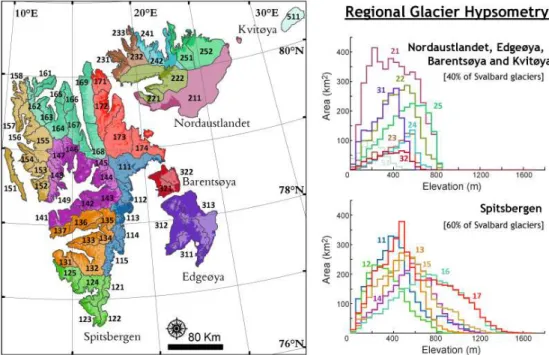
Fig. 2.Regions, primary and secondary drainage basins (i.e. the first three digits of the IDs). The colors depict the primary drainage basins (i.e. the first two digits of the IDs) and correspond to the colors in the glacier hypsometries shown to the right. Glacier hypsometries are extracted from the ASTER GDEM.
glacier basins (Racoviteanu et al., 2009) in the 1990 outlines, forming the GI90 inventory. Finally, the GI00sdataset is
cre-ated from the most recent of either GI90or GIoldby manually
trimming or reshaping the front position and the lateral edges of the glacier tongue to the more recent satellite orthophotos. The basis of the outline reshaping is visual interpretation of the satellite optical images using contrast stretching to aid the delineation of the glacier margin. Outlines were also updated in the upper regions of the glaciers when nunataks appeared or large changes were present due to upper glacier down-wasting, for example from a surge.
The local identification system for individual glaciers is defined hydrologically by the WGI IDs of H93 comprising 5 digits:
– 1st digit represents the division of the archipelago into
5 major regions: (1) Spitsbergen, (2) Nordaustlandet, (3) Barentsøya, (4) Egdeøya, and (5) Kvitøya.
– 2nd digit is the division of each region into primary
drainage basins.
– 3rd digit is the division into secondary drainage basins. – 4th and 5th digits are the number for each individual
glacier.
For example, if a glacier is denoted by 14 204, then the glacier lies in region 1 (Spitsbergen), in major drainage basin 4 (Isfjorden), and in secondary drainage basin 2 (Advent-dalen), and its glacier number is 04 (Longyearbreen). An
overview map of the regions and drainage basins is shown in Fig. 2.
The original H93 glacier identification system required adaptation since a number of individual WGI glacier units in H93 comprised single tongues fed by multiple tributary ice streams that can now be divided into new discrete flow units. Either the old glacier front has retreated and naturally sepa-rated into separate tongues or the tributary glaciers have sig-nificant medial moraines suggesting a natural division of the glacier system. These new independent glacier units retain the original H93 ID, but with additional decimals to identify the individual glacier entities (see Fig. 3). In addition, a few of the flow divides on the 2 larger ice caps have been ad-justed based upon updated information (Sect. 2.3) that was not available in the creation of H93.
Lastly, an inventory requires also definitions of the small-est snow patches and glacierets (Cogley et al., 2011). GI00s
defines glacierets and snow patches as those visually and perennially present in the temporal series of Landsat and ASTER images, the smallest of which is 0.05 km2. H93 de-fines glacierets and snowpatches as perennial snow/ice areas less than 1 km2, and these units were not given specific IDs.
Therefore, these units are labeled in GI00sbased on their
.
80°N
78°N
25°E 15°E 13116
13117.1 13118
13201
13202.1 13202.2 13202.3
13205.2
13205.1
11505
11506
11507
11508
11509
11510
a)
b)
GIold
centerlines
5 km
5 k
m
a) b) GI90
GI00s
widths Elevation
1700
0
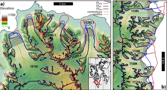
Fig. 3.Examples of the digital inventories from a selection of(a)land-terminating and(b)tidewater glaciers in southern Spitsbergen. Selected
glaciers are shown with their local identification codes, centerlines and glacier tongue widths. Note that only centerlines and tongue widths from the lowest 10% of the centerline of the GI00sare shown.
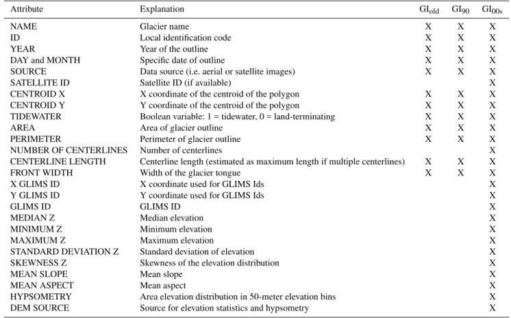
3.3 Glaciological and topographic attributes
For the GI00s inventory, a number of descriptive, glacier
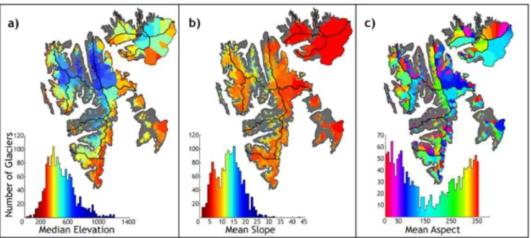
and topographic attributes are extracted for each individual glacier entity, as suggested by Paul et al. (2009). The stan-dard geometric and topographic parameters include polygon area, polygon perimeter, elevation minimum, maximum, me-dian and standard deviation, mean slope and mean aspect. Glacier hypsometries are extracted for 50 m elevation bins from the ASTER GDEM; these are shown in Fig. 2 for the primary drainage basins.
Two additional glaciological parameters are generated for the three inventories: glacier length and the average width of the glacier tongue. At least one centerline is manually digi-tized for each glacier area polygon, from the glacier tongue to the head of the accumulation area. If a single glacier en-tity contains more than one centerline, the maximum length is provided. The centerlines are then used to generate glacier tongue width. Lines perpendicular to the centerline are in-tersected with the glacier outlines for each GI. The glacier tongue or terminus width is then estimated as the average measured width of the lowermost 10 % of the centerline for GI00s. The threshold is chosen visually to best represent the
varying tongue shapes of both small and large glaciers col-lectively. Varying the threshold by 5 % has little effect except for the smallest glaciers with pointy glacier tongue shapes. For GI90and GIold, if the centerline length change is greater
than 10 % of the earlier centerline, the average width along the area of change is used to ensure estimates are represen-tative for the area of change within an epoch. For glaciers containing multiple centerlines, the average front width of all centerlines are provided. For glaciers that have 2 separate tongues corresponding to individual centerlines, the sum of
front widths is given. Glacier tongue widths serve two pur-poses in the inventory. The first is to estimate a calving front width and the second is for change analysis. Examples of the basic geometric structures of the inventories are shown in Fig. 3 and a list of attributes is given in Table 3.
3.4 Glacier change parameters
A common parameter for comparing multi-temporal inven-tories is area change (e.g. Le Bris et al., 2011; Davies and Glasser, 2012), expressed either as mean annual area change or relative change rates as a percentage. Analysis of raw and relative area changes alone is complicated by its depen-dence on glacier area, tongue width and other geometrical parameters. Therefore, we also derive length changes by two methods. First, centerline length change rates are calculated as the difference in centerline length between the invento-ries, divided by the time interval. Second, we use an adap-tation of the “box method” employed in Greenland (Moon and Joughin, 2008; Box and Decker, 2011; Howat and Eddy, 2011), which provides an average change across the glacier tongue rather than a single estimate dependent upon the lo-cation of the centerline. In our approach, an average length change rate is defined as the area change below the GI00s
median elevation divided by the oldest glacier tongue width (as described above) and subsequently by the time interval. We refer to this length change estimate as the “area/width” length change.
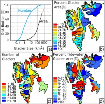
Fig. 4. (a)Glacier number and area distribution of the GI00s inven-tory. E.g. 80 % of the glaciers in the inventory are less than 10 km2, which makes up less than 10 % of the total Svalbard glacierized area.(b)Percent glacierized area of the secondary drainage basins. (c)Number of glaciers within secondary drainage basins reflects an inverse relationship to the percent glacierized area.(d)Percent tidewater glacier area for each secondary drainage basin shows the dominance of tidewater glaciers in Nordaustlandet and the three ice field clusters in Spitsbergen (south, northwest and northeast).
calculated for each glacier’s individual time separation be-tween outlines. Moreover, entire inventory comparisons are made by first calculating the change rates for individual out-lines and then summing to drainage basin or region.
4 Results
4.1 Inventory characteristics
The newest inventory, GI00s, contains 1668 individually
la-beled glacier units (including snowpatch and glacier IDs with a decimal) totaling 33 775 km2, or about 57 % of the total
land area of the archipelago. The distributions of glacier lengths and sizes are approximately log-normal; there are about 350 glaciers (22 % of the inventory) larger than 10 km2
that make up 93 % of the glacier area (Fig. 4a). Similarly, there are 630 glaciers, glacierets and snowpatches smaller than 1 km2that represent 38 % of the inventory and 1 % of the
glacier area (Table 2). Glacier centerline lengths range from 200 m to 60 km, with an average of 4.5 km. A significant log-linear (power-law) relationship exists between glacier area and length, as predicted by theory (Bahr, 1997) and shown with global inventory data (Bahr and Radi´c, 2012).
About 68 % of the glacierized area drains through tidewa-ter calving fronts; their spatial distribution is shown in Fig. 6. The exact number of tidewater glaciers depends on how a glacier is defined. H93 labeled 152 glaciers with a calv-ing front. In GI00s, 197 glaciers with unique identification
codes (including decimals) are characterized as tidewater ter-minating. Twenty-nine of these individually labeled glacier units share the calving glacier tongue with other glaciers but are clearly divided by medial moraines; this leaves 168 calving fronts. Blaszczyk et al. (2009) classified 163 tidewa-ter glaciers, with the difference of 5 glaciers comprising 11 glaciers not classified as tidewater in GI00sand 6 glaciers not
classified as tidewater in Blaszczyk et al. (2009).
Summing the estimated front widths for tidewater glaciers results in a calving front length of 740 km, about half (386 km) of which are tidewater fronts in Spitsbergen. Our glacier tongue widths represent flux gates rather than the pre-cise calving front length. Since lateral edges of many tidewa-ter glaciers in Spitsbergen are grounded on land, our width estimates may often be larger than the active dynamical flux gate of the glacier. The difference with another calving front length estimate of 860 km (Blaszczyk et al., 2009) is due to our smaller front widths on the lobate tongues of ice cap outlet glaciers in Nordaustlandet (215 km), Edgeøya (23 km) and Kvitøya (113 km).
The islands to the east and northeast of Spitsbergen (Edgeøya, Barentsøya and Nordaustlandet) contain the flat-test topographies, and thus glaciers there have lower slopes (Fig. 5b) and are mostly characterized by ice cap geome-tries. Consequently, glacier hypsometries typically feature an abrupt truncation at the highest elevations (Fig. 2). These is-lands contain about 40 % of the glacierized area of Svalbard, with heavy glaciation on Nordaustlandet (60–90 %) and to a lesser extent on Barentsøya/Edgeøya (Fig. 4b). Maximum and median elevations are lower for the ice caps of Bar-entsøya and Edgeøya (Figs. 2 and 5a). About 80 % of the Nordaustlandet glacier area drains through tidewater calving fronts, while only 47 % of the Barentsøya/Edgeøya glacier area is tidewater (Fig. 4d).
Fig. 5.Spatial distribution of(a)median elevation,(b)mean slope in degrees and(c)mean aspect in degrees from north. The color scale is shown as a histogram with the number of glaciers. The distribution of mean slope is slightly bimodal, reflecting two styles of glaciation: the flatter glaciers and icecaps that fill valley floors, and the steeper cirque-style glaciers that sit higher up along the valley walls. The distribution of mean aspect per glacier suggests a dominance of north-facing glaciers; however, histograms of all glacier DEM pixel aspects show a uniform distribution with aspect. The histogram thus reflects the dominance of small glaciers facing northward.
Fig. 6. (a)Distribution of land-terminating and tidewater glaciers in Svalbard. The sum of tidewater glacier front widths within each
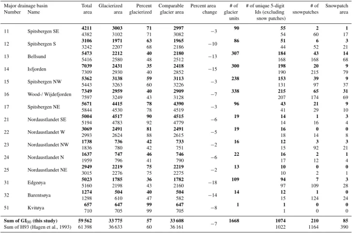
Table 2.Glacier statistics for the major drainage basins of Svalbard for H93 and GI00s(inbold). Total area is the size of the drainage basin, both glacier and land. “Glacierized area” is the total glacierized area in each atlas. Differences in this parameter include glacier change and ommission/commission errors between the datasets. “Comparable glacier area” is the area corresponding to similar IDs in both inventories excluding snow patches and glacierets (see Sect. 3.2). Differences in this parameter include glacier changes and an error associated with delineating glaciers. “Percent area change” is derived from “omparable glacier area”. The number of glacier units is provided only for GI00s as the number of unique 5-digit IDs (no decimals) provides the total number for H93. For GI00s, this is the number of merged integer IDs. Also shown is the number of individual snow patches (GI00sIDs=XXX99.XX) and glaciers less than 1 km2(H93) along with the area sums. All area estimates have unit km2.
Major drainage basin Total Glacierized Percent Comparable Percent area # of # of unique 5-digit # of Snowpatch
Number Name area area glacierized glacier area change glacier Ids (excluding snowpatches area
units snow patches)
11 Spitsbergen SE 4211 3003 71 2997 −3 90 55 2 1
4382 3102 71 3082 54 60 17
12 Spitsbergen S 3106 1971 63 1965 −10 86 51 6 3
3242 2207 68 2186 44 52 21
13 Bellsund 5473 2212 40 2180 −13 307 184 43 14
5416 2580 48 2512 168 168 68
14 Isfjorden 7039 2431 35 2418 −15 300 198 20 9
7309 2930 40 2852 190 215 79
15 Spitsbergen NW 5362 3138 59 3113 −3 238 153 39 9
5443 3263 60 3226 131 97 37
16 Wood-/ Wijdefjorden 7349 2959 40 2909 −7 338 215 65 31
7597 3249 43 3128 207 174 69
17 Spitsbergen NE 5671 4415 78 4390 −3 96 43 21 9
5844 4530 78 4519 41 29 10
21 Nordaustlandet SE 5004 4517 90 4515 −6 19 14 1 3
5194 4783 92 4779 14 16 4
22 Nordaustlandet W 3069 2491 81 2491 −5 19 16 0 0
2993 2624 88 2615 18 14 8
23 Nordaustlandet NW 1738 736 42 733 −2 16 12 3 3
1836 780 42 751 15 92 21
24 Nordaustlandet N 1637 747 46 746 −6 22 16 2 1
1959 796 41 790 17 12 4
25 Nordaustlandet NE 2949 2219 75 2219 −2 13 10 0 0
3015 2276 75 2275 10 2 1
31 Edgeøya 5023 1785 36 1782 −18 109 94 7 3
5160 2198 43 2160 97 109 28
32 Barentsøya 1274 504 40 504 −14 14 12 1 0
1298 610 47 582 15 124 24
51 Kvitøya 657 647 99 647 −8 1 1 0 0
710 705 99 705 1 0 0
Sum of GI00(this study) 59 562 33 775 57 33 608 −
7 1668 1074 210 85
Sum of H93 (Hagen et al., 1993) 61 398 36 633 60 36 161 1022 1164 390
Spitsbergen (Fig. 6), which together drain about 62 % of the Spitsbergen glacierized area. The main tidewater drainage occurs off the eastern and western coastline of Spitsbergen and in Hornsund, Van Keulenfjord, Kongsfjord and Kross-fjord.
4.2 Comparison of complete glacier inventories (H93 vs. GI00s)
This section describes the differences between the only two fully complete glacier inventories of Svalbard, namely H93 and GI00s. The comparison is complicated by both the
varying time spans from which they were derived (Fig. 1) and the lack of raw H93 outlines to control that the up-per glacier boundaries are consistent between the invento-ries. H93 contains 1022 individually labeled glaciers and 1164 non-labeled snow/ice masses less than 1 km2totaling
36 633 km2, or 60 % of the archipelago’s land area (Table 2),
while GI00s contains 1668 individual glacier area polygons,
or∼57 % of the archipelago land area. GI00scontain more
individual units (polygons) due both to glacier retreat and separation, as well as our identification of distinct glacier flow units in glaciers previously classified by a single ID. Thus, GI00sglaciers are combined to their parent single
5-digit integer ID for comparisons. GI00scontain an additional
52 smaller glaciers not formally identified in H93; these we have defined with 5-digit integer IDs that continue from the highest glacier number in each secondary drainage basin. Note that they do not follow the standard counter-clockwise identification sequence of H93.
In terms of snow patches, GI00scontains roughly a
Table 3.List and description of attributes available for each glacier inventory.
Attribute Explanation GIold GI90 GI00s
NAME Glacier name X X X
ID Local identification code X X X
YEAR Year of the outline X X X
DAY and MONTH Specific date of outline X X X
SOURCE Data source (i.e. aerial or satellite images) X X X
SATELLITE ID Satellite ID (if available) X
CENTROID X X coordinate of the centroid of the polygon X X X
CENTROID Y Y coordinate of the centroid of the polygon X X X
TIDEWATER Boolean variable: 1 = tidewater, 0 = land-terminating X X X
AREA Area of glacier outline X X X
PERIMETER Perimeter of glacier outline X X X
NUMBER OF CENTERLINES Number of centerlines X
CENTERLINE LENGTH Centerline length (estimated as maximum length if multiple centerlines) X X X
FRONT WIDTH Width of the glacier tongue X X X
X GLIMS ID X coordinate used for GLIMS Ids X
Y GLIMS ID Y coordinate used for GLIMS Ids X
GLIMS ID GLIMS ID X
MEDIAN Z Median elevation X
MINIMUM Z Minimum elevation X
MAXIMUM Z Maximum elevation X
STANDARD DEVIATION Z Standard deviation of elevation X
SKEWNESS Z Skewness of the elevation distribution X
MEAN SLOPE Mean slope X
MEAN ASPECT Mean aspect X
HYPSOMETRY Area elevation distribution in 50-meter elevation bins X
DEM SOURCE Source for elevation statistics and hypsometry X
in mid- to late summer, and thus were liable to be identified by cartographers as “glacier” in aerial and satellite images. We do not consider these polygons as glaciers and they are not maintained in our GI inventories; however, they are most likely included in the H93 count of glaciers/snow patches
<1 km2and probably are the reason behind the differences
in snowpatches between the inventories.
The difference between comparable areas of H93 and GI00s reveals a glacierized area loss of 7 % (Table 2), or
about 80 km2a−1 for the average 32 yr time span between
the inventories. Area changes are computed at the primary and secondary drainage basin scale (Table 2 and Fig. 6b). This reduces random uncertainties from individual glacier divides and possibly misclassifications (see Sect. 4.4). The smallest relative changes (−2 to −5 %) have occurred in
Nordaustlandet and the largest (−13 to −17 %) in central
Spitsbergen, a region dominated by small glaciers, and Bar-entsøya/Edgeøya (Table 2). These patterns naturally reflect glacier area itself (Figs. 4b and 6b) as described in many other glacier inventory studies (Kääb et al., 2002; Andreassen et al., 2008; Racoviteanu et al., 2008; Bolch et al., 2010; Le Bris et al., 2011) and further complicate spatial and tem-poral change analysis of inventory data.
4.3 Comparison of multi-temporal glacier inventories (GIoldvs. GI90vs. GI00s)
The digital glacier inventories are available for three different times (Fig. 1), with 946 consistent glaciers (∼30 % of the
to-tal Svalbard glacierized area) located in southern and western Spitsbergen. This permits analysis of two time periods, from GIold to GI90 (Epoch 1, which is ∼50 yr on average) and
from GI90 to GI00s(Epoch 2, which is∼17 yr on average).
In sum, these glaciers lost ∼31 km2a−1 (0.26 %a−1)
dur-ing Epoch 1 and∼24 km2a−1(0.23 %a−1) during Epoch 2.
In the following analysis, the sample population is limited to glaciers larger than 2 km2 (406 glaciers) since smaller
glaciers are more prone to interpretation errors related to sea-sonal snow.
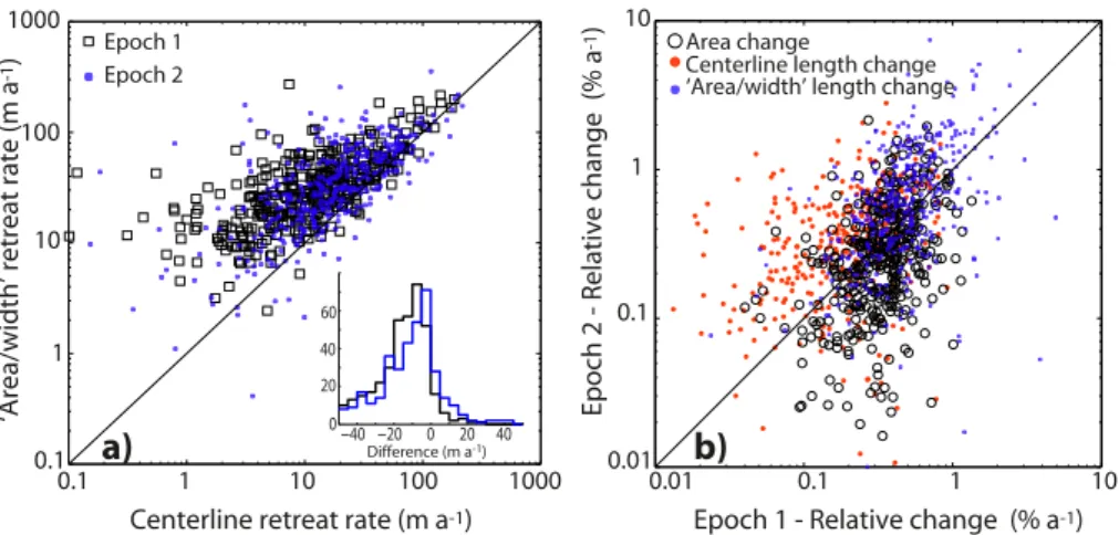
Figure 7a shows centerline length changes and area/width length changes (calculated according to Sect. 3.4). On aver-age, area/width retreat rates are∼10 ma−1larger than
cen-terline retreat rates. This is expected since the area/width length changes are an integrated change that also include lat-eral losses, while the centerline length changes are depen-dent upon one measurement taken along the centerline at the glacier front.
0.01 0.1 1 10 10
0.01 0.1 1
0.1 1 10 100 1000
10
0.1 1 100 1000
‘Area/width’ retreat rate (m a
-1)
Epoch 1 - Relative change (% a-1)
Epoch 2 - Relative change (% a
-1) Area change
‘Area/width’ length change Centerline length change
−40 −20 0 20 40 0
20 40 60
Difference (m a-1)
a)
b)
Epoch 2 Epoch 1
Centerline retreat rate (m a-1)
Fig. 7. (a)Temporal mean retreat rates for Epoch 1 and 2, as estimated from the centerline differences and by the area change divided by
tongue width (“area/width”). The inset shows the histogram of differences between the two retreat rate estimates. The “area/width” retreat rates are larger than the centerline due to both incorporation of lateral losses in the area/width retreat rate estimate and a lack of representative retreat sampling of the centerline.(b)Relative changes during Epoch 1 and Epoch 2 for area changes, centerline length changes and the “area/width” length changes.
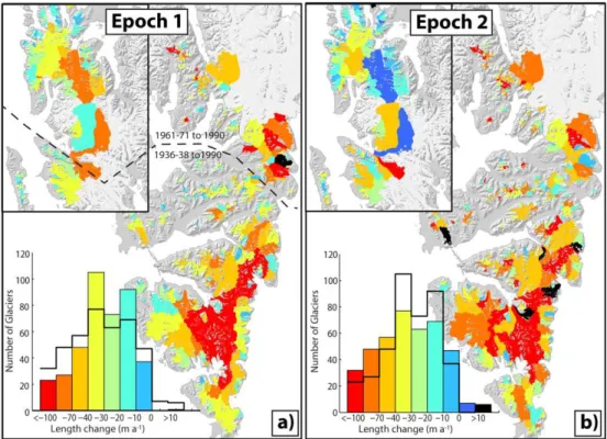
Fig. 8. Length change rates generally vary between 0 and
−150 ma−1, with an average of∼ −40 m a−1and median of −30 m a−1for both epochs. Larger extreme retreat rates exist
(±150–350 ma−1), in most cases related to surge behavior. It
seems the retreat of glaciers has increased, as is apparent in the shift in the distribution of retreat rates towards more nega-tive values in Epoch 2. This is mostly apparent in central and southern Spitsbergen, as compared to northwest Spitsbergen, where average length change rates have remained similar (or even less negative) between the epochs (Fig. 8).
Comparisons between the relative changes of Epoch 1 and Epoch 2 for the area and length changes display varying pat-terns (Fig. 7b). Relative length changes are mainly larger for Epoch 2 than Epoch 1. Similarly to the absolute differ-ences described above (Fig. 7a), relative centerline changes are smaller and vary more than relative area/width length changes. Relative area changes show greater scatter, with many glaciers experiencing larger relative changes during Epoch 1 than Epoch 2. This pattern is opposite that of rel-ative length changes (both centerline and area/width length changes) and is at least partially a result of lateral glacier wastage, which was larger in Epoch 1 than Epoch 2. Nev-ertheless, all relative changes are dependent upon the orig-inal size of the parameter (length or area), and thus spatial and temporal comparisons are hampered by this dependence, which results in heteroscedastic distributions with glacier size (see e.g. Kääb et al., 2002; Bolch et al., 2010).
4.4 Accuracy
Errors in the glacier outlines depend on the images used to delineate glaciers (i.e. their resolution and quality) and sky and ground conditions, and the analyst’s ability to digitize and interpret the imagery. Errors of the latter kind arise both
from the manual interpretation of glacier–land boundaries and from the uncertainty of locating hydrological divides of interconnected ice fields (i.e. based upon surface topogra-phy). Errors in ice field divides are related to the accuracy of the DEM and to the hydrological flow directions derived from it when using automated hydrological GIS algorithms. Interpretation uncertainty may arise, for example, in cases where debris or lateral moraines obscure the glacier outlines, or where seasonal snow in the imagery covers the glacier edge. A manual digitization experiment (Paul et al., 2013) with 20 participants on 24 glaciers resulted in area uncer-tainties (expressed as a relative difference) ranging between 2 and 30 %; the largest errors came from sections of glaciers with heavy debris cover. Manual digitization error was found to be on the order of 1–3 pixels at any vertex; relative er-rors were typically better than 5 %, varying with glacier size and conditions (i.e. debris cover) (Paul et al., 2013). For our digital datasets, we expect errors of this magnitude but also some degree of spatial variability in the uncertainty since, for example, central and north-central areas are less glacierized (i.e. less than 40 % in Fig. 4b) and have larger amounts of debris cover and/or ice-cored moraines.
Glacier outlines for H93 are not digitally available, but they are based on many of the same topographic maps as GIoldfrom which we have derived glacier divides
Fig. 8.Average length change rates calculated using the area/width method between(a)GIoldand GI90and(b)GI90and GI00s. The inset map is a section of northwest Spitsbergen. The histogram insets show the number of glaciers for each color used in the map. The straight bar line in the histograms are of the alternate epoch for comparison. The distribution of Epoch 2 length changes is more negative than that of Epoch 1.
drainage divides or from the inclusion or exclusion of lateral moraines, which impacts the relative error more heavily than the smaller random errors introduced in digitization (as de-scribed in Paul et al., 2013).
We define the individual glacier area error as the 95 % con-fidence interval of the Studenttdistribution, about 16 %, but
note that the relative error is dependent upon glacier size as well (Kääb et al., 2002; Bolch et al., 2010; Paul et al., 2013), with smaller glaciers having larger relative errors. The bulk of the glaciers have errors less than 5 %, similar to other in-ventories (Paul et al., 2002; Bolch et al., 2010; Gjermundsen et al., 2011; Rastner et al., 2012). The error may be largely systematic at the individual glacier scale but is random at the regional or inventory-wide scale; i.e. the uncertainty of the drainage divides is cancelled. A rough conservative estimate for the error of the entire glacierized area of Svalbard is 1– 2 % (∼500 km2).
Finally, we simulate a 16 % error on the area changes and on the glacier tongue widths to estimate a sensitivity to and the precision of our area/width length changes. For the entire population of changes from Epoch 2, the residuals between the original length changes and those calculated with 16 % differences in the area changes and widths separately result in a error distribution approximated by a Studenttwith 95 % of the residuals contained within±10 ma−1. Combining both
uncertainties from area changes and glacier tongue width
es-−600 −40 −20 0 20 40 60
2 4 6
8
Count
Error (%)
Gaussian
Student-t
Fig. 9.Distribution of area errors between H93 and GIoldfor all
glaciers mapped in the same year, as a percent of the glacier area showing Gaussian and Studentt distributions fit to the data. The
heavier tails of the Studenttdistribution reflect the effect of larger
timates by standard error propagation (root sum of squares) results in an error of 14 ma−1. About 80 % of the observed
length change rates in Epoch 1 and 2 (Fig. 8) are above this uncertainty.
All of the change parameters are sensitive to bias in-duced by interpretation uncertainty. In particular, the deci-sion whether to include or exclude lateral moraines within the glacier area needs to be consistent within multi-temporal inventories. In Svalbard, glacier ice may exist beneath these lateral moraines (F. Navarro and A. Martín-Español, per-sonal communication, 2013). Our inventories exclude lat-eral moraines by adopting a visual definition for delineating glaciers based on spectral appearance. Without widespread ground truth information about ice below debris, it is not possible to quantify potential error introduced. In addition, the decision whether to include or exclude lateral moraines is subjective and dependent upon the purpose of the glacier area outline. In Svalbard, the retreat of glaciers commonly occurs at the front rather than the sides; accordingly exclu-sion of the lateral moraines seems appropriate for studies of glacier extent changes. Alternately, using glacier area for vol-ume estimation may require their inclusion (Radi´c and Hock, 2010; Huss and Farinotti, 2012; Martín-Español et al., 2013).
5 Discussion
Our new glacier inventory of Svalbard, GI00s, can be used
to extract spatial data reflecting topography and climatol-ogy of the archipelago. Median glacier elevation (Fig. 5a) is a characteristic of an individual glacier’s hypsometry that is highly correlated with the equilibrium line altitude, or ELA (Braithwaite and Raper, 2009). The median elevation has been used for developing concepts of “glaciation limits” and proxies for the long-term ELA, the patterns of which sug-gest an inverse relation to the precipitation regime (Østrem, 1966; Schiefer et al., 2008). In Svalbard, spatial patterns of median glacier elevation have previously been used to infer spatial variability of the ELA (Hagen et al., 2003) and pre-cipitation (Hisdal, 1985; Hagen et al., 1993; Winther et al., 1998; Sand et al., 2003). In central Spitsbergen, the spatial patterns of the median elevation match closely the mapped 1990 late summer snow line (a proxy for the ELA) distribu-tion (Humlum, 2002). On Austfonna, snow depth variability shows a clear northwest–southeast gradient (Taurisano et al., 2007; Dunse et al., 2009) due to the predominance of precip-itation coming from the Barents Sea (Schuler et al., 2007). This is reflected in lower median glacier elevations towards the southeast and higher towards the northwest (Fig. 5a). Spatial patterns of median glacier elevation similarly reflect the annual total number of melt days and summer melt on-set as estimated from QuikSCAT scatterometry (Rotschky et al., 2011). The spatial patterns of median elevation over the archipelago reflect the local degree of glaciation, which is dependent upon both the terrain and the long-term regional
climatological patterns that result in spatial variations of ac-cumulation and ablation (mass balance) over the terrain sur-face. Higher glacier median elevations occur in the central drier regions of Spitsbergen and correspond to areas that ex-perience lower average annual melt days, which could imply lower mass turnover. Moreover, these areas have lower per-cent glaciation and larger number of glaciers in the inventory (Fig. 4).
A glacier inventory represents a snapshot of the glacier geometrical extent, typically at a single point in time. Our glacier inventories are generally not a single point in time but cover a range of times, though each glacier outline has a distinct time stamp. Comparing multiple glacier invento-ries through time allows investigation of changes in some of the basic glacier geometry parameters. Changes in glacier area and length reflect the glacier’s total response (Oerle-mans, 2001). At smaller regional scales, area and length changes of individual glaciers manifest themselves differ-ently to the presumably more or less uniform driving cli-mate signal, due to variable glacier response times. Glacier response time is proportional to thickness and inversely pro-portional to the ablation rate at the terminus (e.g. Jóhan-nesson et al., 1989), such that front positions of small thin glaciers respond more quickly to the same climate change signal. Above a critical glacier size (i.e. larger glaciers) and holding all mass balance gradients similar, theory and mod-eling experiments predict a decreasing response time, with increasing glacier size resulting from the dynamic controls on response time (Bahr et al., 1998; Pfeffer et al., 1998). Estimated response times for Svalbard glaciers are in the range of decades to centuries, implying that observed front position changes still contain signals from earlier climatic events – especially true for Epoch 1. Epoch 2 changes may reflect climate changes during both Epoch 1 and Epoch 2. In Svalbard, the frequent surging behavior of many Svalbard glaciers (Lefauconnier and Hagen, 1991; Hagen et al., 1993; Hamilton and Dowdeswell, 1996; Jiskoot et al., 2000; Sund et al., 2009) complicates reconstructions of past climate from change records (as in Oerlemans, 2005). Finally, since each inventory represents a single glacier snapshot, the variation in temporal separation between inventories (epoch length), and its relation with the timing of each individual glaciers response will influence the observed average change rates. Enhanced interpretation of these changes may be possible with the inclusion of an accurate surge glacier inventory. This was not completed for this study due to insecurities in defin-ing exactly which glaciers have fully surged or only partially surged (Sund et al., 2009) especially over the decadal time period of this study where glaciers that have surged may not be visible in the area changes given the long time span be-tween the inventories. Future work should focus on generat-ing such an inventory.
Epoch 1 (m a-1)
1000 100
10 1
1000
100
10
1
1000 100
10 1
1000
100
10
1
Land-terminating glaciers
Tidewater glaciers
0 25 50
Epoch 1 (m a-1)
Epoch 2 (m a
-1)
Epoch 2 (m a
-1)
-25
-50
A
v
er
age r
etr
ea
t r
a
te diff
er
enc
e bet
w
een epoch 1 and 2 (m a
-1
)
Fig. 10.Annual average length changes calculated using the “area/width” method for land-terminating (left) and tidewater (right) glaciers
for Epoch 1 vs. Epoch 2. Colors represent the difference in average retreat rates between the epochs. Black diamonds are glaciers that have advanced in either Epoch 1 or 2. Symbols in the maps (bottom) are identical to those in the scatter plots (top). In the scatter plots, points below the 1:1 line are glaciers that have experienced smaller retreat rates in Epoch 2 (blue), while points above the line are glaciers that have experienced greater retreat in Epoch 2 (red). Note the log scale of the scatter plot and linear color scale in the difference of average retreat rates. The size of the symbol is a log scale of the glacier size.
60 % of the differenced retreat rates are greater than the 95 % confidence interval of 10 ma−1(see Sect. 4.4). For the entire
sample and the significant subsample,∼60 % of the glaciers
have experienced larger retreat rates in Epoch 2, apparent as a shift in the histograms between the two epoch-averaged re-treat rates (Fig. 8). The spatial patterns of Fig. 10 suggest a potential regional trend with greater retreat in Epoch 2 in southern Spitsbergen and less so in northwest Spitsber-gen. Moreover, slight clustering or spatial autocorrelation in the retreat rate changes between the epochs is present. This may reflect the geometrical similarity between neigh-boring glaciers that is dictated by the topography and the more or less uniform driving climate signal. On top of the apparent clustering, larger outliers are present, with some neighboring glaciers having opposing (either positive or neg-ative) differenced retreat rates. These local outliers represent
variability in the individual glacier responses to the driving climate and/or the effect of past and present surge glaciers and their surge history in relation to the timing of the in-ventories. Combination with additional parameters such as geodetic volume changes (e.g. Nuth et al., 2007), estimated glacier volumes and thicknesses or terminus mass balance rates (Haeberli and Hoelzle, 1995; Hoelzle et al., 2007) will aid interpretations related to response times and climate.
(Sect. 3.4). Area/width length changes are larger than the centerline length changes (Fig. 7a) as they integrate the entire front position change (including lateral changes), while cen-terline changes are one single measurement of the front. The area/width method minimizes area-related errors from uncer-tain upper glacier boundaries by limiting the analysis to area change below the median glacier elevation and may be fully automated allowing easy retrieval from repeat inventories.
Using the entire sample of glaciers that exist consis-tently in GIold, GI90 and GI00s, the total area change rates
and relative area change rates are 22 % smaller in Epoch 2 (−24 km2a−1, 0.23 %a−1) than in Epoch 1 (−31 km2a−1,
0.26 %a−1). Alternately, summing the area/width
(center-line) length changes for all glaciers results in 14 (30) % more negative length changes during Epoch 2 (−29.5 (−15.3) km
a−1) as compared to Epoch 1 (−25
.6 (−11.9) km a−1). Thus,
while area change rates were larger in Epoch 1, the length change rates were larger in Epoch 2, which is similarly re-flected in Fig. 7b. The total summed change rates of glacier tongue width during Epoch 1 is−2.2 kma−1as opposed to −1.4 kma−1for Epoch 2. General reduction in glacier area
loss rates in Epoch 2 is probably a geometrical effect of de-creased lateral wastage of the glacier tongues, despite the faster average retreat rates experienced in Epoch 2.
6 Conclusions
This study describes the creation of a consistent multi-temporal digital glacier inventory of the Svalbard archipelago, based on the structure of the previous in-ventory (Hagen et al., 1993). Our new digital inin-ventory is based on historic data that are available digitally and then progressively updated through time to maintain consistency between the glacier outlines. This required modification of the identification system already in place (WGMS, 1989; Hagen et al., 1993) for glaciers that have retreated and separated. Moreover, the newest inventory also includes snowpatches and glacierets that are less than 1 km2 as
identified in available cloud-free SPOT, ASTER and Landsat images. GI00s, the present digital inventory, coheres to both
GLIMS and WGI standards (with slight modifications) and has been incorporated into the Randolph Glacier Inven-tory (Arendt et al., 2012) and the GLIMS database. The inventories may also be downloaded from the Norwegian Polar Institute data archive (http://data.npolar.no/dataset/ 89f430f8-862f-11e2-8036-005056ad0004).
In total, the GI00s inventory of glaciers in Svalbard
con-tains 1668 individual glacier units, for a total glacierized area of 33 775 km2, or∼57 % of the archipelago. About 60 % of
the glacierized area is on Spitsbergen and 40 % on the is-land to the east-northeast. Between 168 and 197 tidewater glaciers (depending on how a single tidewater glacier is de-fined) drain 68 % of the glacierized area through a summed glacier terminus width of about 740 km. The glacierized area
has decreased by an average of∼80 km2a−1 over the past ∼30 yr, a reduction of 7 %. For a sample of∼400 glaciers
in south and west Spitsbergen, glacier retreat was greater af-ter 1990 (Epoch 2), while area change rates were greaaf-ter in the decades before 1990 (Epoch 1), corresponding to more lateral wastage in the early period.
We suggest that reducing the dimensions of area change to a length scale may provide a more useful parameter for spatio-temporal analysis of change signals. This falls in line with previous investigations (Raup et al., 2009) and may en-hance the use and incorporation of glacier inventory changes, for example, into numerical models (e.g. Oerlemans, 1997; Vieli et al., 2001; Nick et al., 2009) and/or temperature re-constructions (Oerlemans, 2005; Leclercq and Oerlemans, 2012). The spatio-temporal variability of the length change rates suggests response time variation that requires further investigation. With increased accuracy and capability to au-tomatically generate glacier inventories at higher tempo-ral resolutions using satellite data, the generation of repeat glacier inventory changes in the form of area, tongue width and length changes will become an important observational dataset for future glacier–climate studies.
Appendix A
ASTER GDEM pre-processing and assessment
The ASTER GDEM Version 2 is a merged composite of multi-temporal DEMs from individual ASTER stereo im-age pairs. As with version 1, version 2 contains a quality mask that indicates the number of images used for deter-mining each pixel elevation. Individual DEMs are automat-ically generated following Fujisada et al. (2005), and then merged by averaging the data stack at similar locations af-ter filaf-tering pixels that are 40 m higher than the mean (Fu-jisada et al., 2012). One improvement to version 1 is an im-proved resolution resulting from a smaller matching template in the original parallax determination of the DEM generation (Tachikawa et al., 2011). Version 2 displays a single distinct misalignment when compared to ICESat and SPOT-SPIRIT DEMs despite the apparent lack of co-registration during the DEM stacking process (Fujisada et al., 2012) and relatively good co-registration documented in the final validation report (Tachikawa et al., 2011).
Fig. A1. (a)Hillshades draped by elevation for the original ASTER GDEM,(b)the Fourier-filtered GDEM, and(c)a 2008 SPOT5-HRS DEM.(d)The differences between the filtered GDEM and the SPOT DEM with the black areas containing correlations that are less than 40.(e)and(f)show normalized histograms (yaxis as percentage of pixels) of elevation differences (xaxis in meters) for land and glaciers,
respectively, for the DEMs and ICESat. In the legend of(e), “GDEMo” and “GDEMf” are the original and filtered GDEM, respectively. (g)and(h)show two individual ICESat profiles over higher-elevation glacier regions (typical for low visible contrast areas) from 27 May 2005 and 19 March 2008, respectively, with their differences to the three DEMs. The thick brown line shows the topography, while the other colored lines correspond to the labels presented in(e).
frequency of the bumpy glacier surface seen in Fig. A1a. A single frequency of the artifacts was not practically de-terminable for use in a frequency stop filter due to the sim-ilarity of the artifacts with the natural glacier topographic fluctuations and the frequency of off-glacier terrain. There-fore, we choose to apply a standard low-pass filter in the fre-quency domain, using a Hanning window. The set of param-eters (order and frequency cut-off) is chosen by minimizing the standard deviation of the glacier differences between the GDEM and ICESat. Post-filtered topography was not sen-sitive to small fluctuations in the parameters. The filtered GDEM (Fig. A1b) shows improvement over smooth glaciers (Fig. A1e) but resembles a downgraded (lower resolution) product over the rougher surrounding terrain (Fig. A1f). Most of the higher-frequency noise is removed (Fig. A1g), though the lower-frequency bumps remain, with maximum
differences of up to 50–60 m (Fig. A1h). Therefore, our fi-nal post-processed GDEM is a compilation of the Fourier-filtered glacier surface with a median block Fourier-filtered non-glacier surface.
Acknowledgements. We would like to thank the Norwegian Polar
by the Nordic Top-level Research Initiative. The SPOT5-HRS DEMs and orthophotos were obtained through the IPY-SPIRIT program (Korona et al., 2009) ©CNES 2008 and SPOT Image 2008, all rights reserved. The ASTER L1B data were obtained within the framework of the Global Land Ice Measurements from Space project (GLIMS) through the online data pool at the NASA Land Processes Distributed Active Archive Center (LP DAAC), USGS/Earth Resources Observation and Science (EROS) Center, Sioux Falls, South Dakota. Landsat images are downloaded from http://glovis.usgs.gov/. NASA’s ICESat GLAS data were obtained from NSIDC. The ASTER GDEM [v2] is a product of METI and NASA and was downloaded from the LPDAAC.
Author Contributions. J. Kohler, M. König and C. Nuth
re-alized the design of the inventory. M. König, G. Moholdt, R. Petterson and C. Nuth contributed data to the inventory. A. von Deschwanden prepared submission of the inventory to the GLIMS database. J. Kohler, J. O. Hagen, A. Kääb and C. Nuth developed concepts to the study and methodologies. C. Nuth prepared the final data and wrote the original manuscript. All authors wrote and edited the final paper.
Edited by: J. L. Bamber
References
Ahlmann, H. W., Eriksson, B. E., Ångström, A., and Rosenbaum, L.: Scientific Results of the Swedish-Norwegian Arctic Expedi-tion in the Summer of 1931, Part IV–VIII, Geogr. Ann., 15, 73– 216, http://www.jstor.org/stable/519460, 1933.
Andreassen, L. M., Paul, F., Kääb, A., and Hausberg, J. E.: Landsat-derived glacier inventory for Jotunheimen, Norway, and deduced glacier changes since the 1930s, The Cryosphere, 2, 131–145, doi:10.5194/tc-2-131-2008, 2008.
Arendt, A., Bolch, T., Cogley, J., Gardner, A., Hagen, J.-O., Hock, R., Kaser, G., Pfeffer, W., Moholdt, G., Paul, F., Radic, V., An-dreassen, L., Bajracharya, S., Beedle, M., Berthier, E., Bham-bri, R., Bliss, A., Brown, I., Burgess, E., Burgess, D., Cawk-well, F., Chinn, T., Copland, L., Davies, B., Angelis, H. D., Dol-gova, E., Filbert, K., Forester, R., Fountain, A., Frey, H., Gif-fen, B., Glasser, N., Gurney, S., Hagg, W., Hall, D., Haritashya, U., Hartmann, G., Helm, C., Herreid, S., Howat, I., Kapustin, G., Khromova, T., Kienholz, C., Koenig, M., Kohler, J., Kriegel, D., Kutuzov, S., Lavrentiev, I., LeBris, R., Lund, J., Manley, W., Mayer, C., Miles, E., Li, X., Menounos, B., Mercer, A., Moelg, N., Mool, P., Nosenko, G., Negrete, A., Nuth, C., Pettersson, R., Racoviteanu, A., Ranzi, R., Rastner, P., Rau, F., Raup, B., Rich, J., Rott, H., Schneider, C., Seliverstov, Y., Sharp, M., Sigurds-son, O., Stokes, C., Wheate, R., Winsvold, S., Wolken, G., Wy-att, F., and Zheltyhina, N.: Randolph Glacier Inventory [v2.0]: A Dataset of Global Glacier Outlines, Tech. rep., Global Land Ice Measurements from Space, 2012.
AST14DMO: On Demand Digital Elevation Model & Registered Radiance at the Sensor – Orthorectified, Tech. rep., NASA Land Processes Distributed Active Archive Center (LP DAAC), USGS/Earth Resources Observation and Science (EROS) Center, Sioux Falls, South Dakota, 2010.
Bahr, D. B.: Width and length scaling of glaciers, J. Glaciol., 43, 557–562, 1997.
Bahr, D. B. and Radi´c, V.: Significant contribution to total mass from very small glaciers, The Cryosphere, 6, 763–770, doi:10.5194/tc-6-763-2012, 2012.
Bahr, D. B., Pfeffer, W. T., Sassolas, C., and Meier, M. F.: Response time of glaciers as a function of size and mass balance: 1. The-ory, J. Geophys. Res., 103, 9777–9782, doi:10.1029/98JB00507, 1998.
Blaszczyk, M., Jania, J. A., and Hagen, J. O.: Tidewater glaciers of Svalbard: Recent changes and estimates of calving fluxes, Pol. Polar Res., 30, 85–142, 2009.
Bolch, T., Menounos, B., and Wheate, R.: Landsat-based inventory of glaciers in western Canada, 1985–2005, Remote Sens. Envi-ron., 114, 127–137, doi:10.1016/j.rse.2009.08.015, 2010. Box, J. E. and Decker, D. T.: Greenland marine-terminating
glacier area changes: 2000-2010, Ann. Glaciol., 52, 91–98, doi:10.3189/172756411799096312, 2011.
Braithwaite, R. and Raper, S.: Estimating equilibrium-line altitude (ELA) from glacier inventory data, Ann. Glaciol., 50, 127–132, doi:10.3189/172756410790595930, 2009.
Cogley, J., Hock, R., Rasmussen, L., Arendt, A., Bauder, A., Braith-waite, R., Jansson, P., Kaser, G., Möller, M., Nicholson, L., and Zemp, M.: Glossary of Glacier Mass Balance and Related Terms, IHP-VII Technical Documents in Hydrology No. 86„ Tech. rep., IACS Contribution No. 2, UNESCO-IHP, Paris., 2011.
Cogley, J. G.: A more complete version of the World Glacier Inven-tory, Ann. Glaciol., 50, 32–38, 2009.
Davies, B. and Glasser, N.: Accelerating shrinkage of Patagonian glaciers from the Little Ice Age (AD 1870) to 2011, J. Glaciol., 58, 1363–1384, 2012.
Dowdeswell, J. A., Benham, T. J., Strozzi, T., and Hagen, J. O.: Ice-berg calving flux and mass balance of the Austfonna ice cap on Nordaustlandet, Svalbard, J. Geophys. Res.-Earth, 113, F03022, doi:10.1029/2007JF000905, 2008.
Dunse, T., Schuler, T. V., Hagen, J. O., Eiken, T., Brandt, O., and Høgda, K. A.: Recent fluctuations in the extent of the firn area of Austfonna, Svalbard, inferred from GPR, Ann. Glaciol., 50, 155–162, doi:10.3189/172756409787769780, 2009.
Førland, E. J., Benestad, R., Hanssen-Bauer, I., Haugen, J. E., and Skaugen, T. E.: Temperature and Precipitation Development at Svalbard 1900–2100, Advances in Meteorology, 2011, 893790, doi:10.1155/2011/893790, 2011.
Frey, H. and Paul, F.: On the suitability of the SRTM DEM and ASTER GDEM for the compilation of topographic parameters in glacier inventories, Int. J. Appl. Earth Obs., 18, 480–490, doi:10.1016/j.jag.2011.09.020, 2012.
Fujisada, H., Bailey, G., Kelly, G., Hara, S., and Abrams, M.: ASTER DEM performance, IEEE T. Geosci. Remote, 43, 2707– 2714, doi:10.1109/TGRS.2005.847924, 2005.
Fujisada, H., Urai, M., and Iwasaki, A.: Technical Methodology for ASTER Global DEM, IEEE T. Geosci. Remote, 50, 3725–3736, 2012.
Gjermundsen, E., Mathieu, R., Kaab, A., Chinn, T., Fitzharris, B., and Hagen, J.: Assessment of multispectral glacier mapping methods and derivation of glacier area changes, 19782002, in the central Southern Alps, New Zealand, from ASTER satellite data, field survey and existing inventory data, J. Glaciol., 57, 667–683, doi:10.3189/002214311797409749, 2011.
mountain glaciers: A pilot study with the European Alps, Annals of Glaciology: Proceedings of the International Symposium On the Role of the Cryosphere In Global Change, Columbus Ohio 21 August 1994, , 1995.
Hagen, J. O., Liestøl, O., Roland, E., and Jørgensen., T.: Glacier atlas of Svalbard and Jan Mayen, Norwegian Polar Institue, Oslo, 1993.
Hagen, J. O., Melvold, K., Pinglot, F., and Dowdeswell, J. A.: On the net mass balance of the glaciers and ice caps in Svalbard, Norwegian Arctic, Arct. Antarct. Alp. Res., 35, 264–270, doi:10.1657/1523-0430(2003)035[0264:OTNMBO]2.0.CO;2, 2003.
Hamilton, G. and Dowdeswell, J.: Controls on glacier surging in Svalbard, J. Glaciol., 42, 157–168, 1996.
Hisdal, V.: Geography of Svalbard, vol. 2, Norwegian Polar Institue, Oslo, 1985.
Hoelzle, M., Chinn, T., Stumm, D., Paul, F., Zemp, M., and Haeberli, W.: The application of glacier inventory data for estimating past climate change effects on mountain glaciers: A comparison between the European Alps and the South-ern Alps of New Zealand, Global Planet. Change, 56, 69–82, doi:10.1016/j.gloplacha.2006.07.001, 2007.
Howat, I. M. and Eddy, A.: Multi-decadal retreat of Green-land’s marine-terminating glaciers, J. Glaciol., 57, 389–396, doi:10.3189/002214311796905631, 2011.
Humlum, O.: Modelling late 20th-century precipitation in Nor-denskiöld Land, Svalbard, by geomorphic means, Norsk Geogr. Tidsskr., 56, 96–103, 2002.
Huss, M. and Farinotti, D.: Distributed ice thickness and volume of all glaciers around the globe, J. Geophys. Res., 117, F04010, doi:10.1029/2012JF002523, 2012.
James, T. D., Murray, T., Barrand, N. E., Sykes, H. J., Fox, A. J., and King, M. A.: Observations of enhanced thinning in the up-per reaches of Svalbard glaciers, The Cryosphere, 6, 1369–1381, doi:10.5194/tc-6-1369-2012, 2012.
Jiskoot, H., Murray, T., and Boyle, P.: Controls on the distribu-tion of surge-type glaciers in Svalbard, J. Glaciol., 46, 412–422, doi:10.3189/172756500781833115, 2000.
Jóhannesson, T., Raymond, C., and Waddington, E.: Time-scale for adjustment of glaciers to changes in mass balance, J. Glaciol., 35, 355–369, 1989.
Kääb, A., Paul, F., Maisch, M., Hoelzle, M., and Haeberli, W.: The new remote-sensing-derived Swiss glacier inventory: II. First re-sults, Annals of Glaciology, Vol 34, 2002, 34, Int. Glaciol. Soc., NASA, US Natl. Sci. Fdn., doi:10.3189/172756402781817473, 2002.
Kohler, J., James, T. D., Murray, T., Nuth, C., Brandt, O., Barrand, N. E., Aas, H. F., and Luckman, A.: Acceleration in thinning rate on western Svalbard glaciers, Geophys. Res. Lett., 34, L18502, doi:10.1029/2007GL030681, 2007.
König, M., Nuth, C., Kohler, J., Moholdt, G., and Pettersen, R.: Global Land Ice Measurements from Space, chap. A Digitial Glacier Database for Svalbard, p. Ch. 10, Praxis-Springer, 2013. Korona, J., Berthier, E., Bernard, M., Rémy, F., and Thouvenot, E.: SPIRIT. SPOT 5 stereoscopic survey of Polar Ice: Reference Images and Topographies during the fourth International Polar Year (2007–2009), ISPRS Journal of Photogrammetry and Re-mote Sensing, 64, 204–212, doi:10.1016/j.isprsjprs.2008.10.005, 2009.
Le Bris, R., Paul, F., Frey, H., and Bolch, T.: A new satellite-derived glacier inventory for western Alaska, Ann. Glaciol., 52, 135–143, doi:10.3189/172756411799096303, 2011.
Leclercq, P. and Oerlemans, J.: Global and hemispheric temperature reconstruction from glacier length fluctuations, Clim. Dynam., 38, 1065–1079, doi:10.1007/s00382-011-1145-7, 2012. Lefauconnier, B. and Hagen, J. O.: Surging and calving glaciers in
Eastern Svalbard, vol. 116, Norsk polarinstitutt, Oslo, 1991. Martín-Español, A., Vasilenko, E., Navarro, F., Otero, J., Lapazaran,
J., Lavrentiev, I., Macheret, Y., Machío, F., and Glazovsky, A.: Ice volume estimates from ground-penetrating radar surveys, western Nordenskiöld Land glaciers, Svalbard., Ann. Glaciol. 54, 211–217, 2013.
Moholdt, G. and Kääb, A.: A new DEM of the Austfonna ice cap by combining differential SAR interferometry with ICESat laser altimetry, Polar Res., 31, 18460, doi:10.3402/polar.v31i0.18460, 2012.
Moon, T. and Joughin, I.: Changes in ice front position on Green-land’s outlet glaciers from 1992 to 2007, J. Geophys. Res., 113, F02022, doi:10.1029/2007JF000927, 2008.
Müller, F., Caflisch, T., and Müller, G.: Instructions for Compilation and Assemblage of Data for a World Glacier Inventory, Tech. rep., ETH Zürich.Temporary Technical Secretariat for the World Glacier Inventory., Z"urich, 1977.
Nick, F. M., Vieli, A., Howat, I. M., and Joughin, I.: Large-scale changes in Greenland outlet glacier dynamics triggered at the ter-minus, Nat. Geosci., 2, 110–114, doi:10.1038/ngeo394, 2009. Nordli, Ø. and Kohler, J.: The early 20th century warming – Daily
observations at Grønfjorden and Longyearbyen on Spitsbergen, Tech. rep., Norwegian Meteorological Institue, Oslo, 2004. Nuth, C. and Kääb, A.: Co-registration and bias corrections of
satel-lite elevation data sets for quantifying glacier thickness change, The Cryosphere, 5, 271–290, doi:10.5194/tc-5-271-2011, 2011. Nuth, C., Kohler, J., Aas, H. F., Brandt, O., and Hagen,
J. O.: Glacier geometry and elevation changes on Svalbard (1936–90): a baseline dataset, Ann. Glaciol., 46, 106–116, doi:10.3189/172756407782871440, 2007.
Oerlemans, J.: A flowline model for Nigardsbreen, Norway: projec-tion of future glacier length based on dynamic calibraprojec-tion with the historic record, Ann. Glaciol., 24, 24, 382–389, 1997. Oerlemans, J.: Glaciers and climate change, Balkema Publ., Lisse,
2001.
Oerlemans, J.: Extracting a Climate Signal from 169 Glacier Records, Science, 308, 675–677, doi:10.1126/science.1107046, 2005.
Østrem, G.: The Height of the Glaciation Limit in Southern British Columbia and Alberta, Geogr. Ann. A, 48, 126–138, http://www. jstor.org/stable/520522, 1966.
Paul, F., Kaab, A., Maisch, M., Kellenberger, T., and Hae-berli, W.: The new remote-sensing-derived swiss glacier inventory: I. Methods, Ann. Glaciol., 34, 355–361, doi:10.3189/172756402781817941, 2002.
Paul, F., Barry, R., Cogley, J., Frey, H., Haeberli, W., Ohmura, A., Ommanney, C., Raup, B., Rivera, A., and Zemp, M.: Recommendations for the compilation of glacier inven-tory data from digital sources, Ann. Glaciol., 50, 119–126, doi:10.3189/172756410790595778, 2009.