www.the-cryosphere.net/10/65/2016/ doi:10.5194/tc-10-65-2016
© Author(s) 2016. CC Attribution 3.0 License.
Comparison of multiple glacier inventories with a new inventory
derived from high-resolution ALOS imagery in the Bhutan
Himalaya
H. Nagai1, K. Fujita2, A. Sakai2, T. Nuimura3, and T. Tadono1
1Earth Observation Research Center, Japan Aerospace Exploration Agency, Tsukuba, Japan 2Graduate School of Environmental Studies, Nagoya University, Nagoya, Japan
3Faculty of Risk and Crisis Management, Chiba Institute of Science, Choshi, Japan Correspondence to:H. Nagai ([email protected])
Received: 21 January 2014 – Published in The Cryosphere Discuss.: 25 February 2014 Revised: 30 November 2015 – Accepted: 5 December 2015 – Published: 18 January 2016
Abstract.Digital glacier inventories are invaluable data sets for revealing the characteristics of glacier distribution and for upscaling measurements from selected locations to entire mountain ranges. Here, we present a new inventory of Ad-vanced Land Observing Satellite (ALOS) imagery and com-pare it with existing inventories for the Bhutan Himalaya. The new inventory contains 1583 glaciers (1487±235 km2),
thereof 219 debris-covered glaciers (951±193 km2) and 1364 debris-free glaciers (536±42 km2). Moreover, we pro-pose an index for quantifying consistency between two glacier outlines. Comparison of the overlap ratio demon-strates that the ALOS-derived glacier inventory contains de-lineation uncertainties of 10–20 % which depend on glacier size, that the shapes and geographical locations of glacier outlines derived from the fourth version of the Randolph Glacier Inventory have been improved in the fifth version, and that the latter is consistent with other inventories. In terms of whole glacier distribution, each data set is domi-nated by glaciers of 1.0–5.0 km2 area (31–34 % of the to-tal area), situated at approximately 5400 m elevation (nearly 10 % in 100 m bin) with either north or south aspects (22 and 15 %). However, individual glacier outlines and their area exhibit clear differences among inventories. Further-more, consistent separation of glaciers with inconspicuous termini remains difficult, which, in some cases, results in different values for glacier number. High-resolution imagery from Google Earth can be used to improve the interpretation of glacier outlines, particularly for debris-covered areas and steep adjacent slopes.
1 Introduction
assessment is actually not recommended without adequate quality control.
A glacier inventory containing delineated outlines is a fun-damental asset for assessing glacier change in these remote and extensive mountain regions. Existing glacier inventories for the Himalayas include those of the International Cen-tre for Integrated Mountain Development (ICIMOD; Mool et al., 2001), the project of Glacier Area Mapping for Dis-charge from the Asian Mountains (GAMDAM; Nuimura et al., 2015), and the Chinese Glacier Inventory (Guo et al., 2015) of the Chinese Academy of Science. Subsequently, parts of each have been included in a global glacier inven-tory compiled by the Randolph Consortium, termed the Ran-dolph Glacier Inventory (RGI) (Pfeffer et al., 2014). Several studies have utilised these data sets to clarify recent glacier change (e.g. Vaughan et al., 2013; Bajracharya et al., 2014a, b), glacier lake evolution (Gardelle et al., 2011), and rela-tionships between precipitation and the distribution of glacier elevations (Sakai et al., 2015). The RGI was designed for and applied in several large- to global-scale assessments and modelling studies in support of IPCC AR5 (Vaughan et al., 2013), including past and future global sea level rise (Gardner et al., 2013; Radi´c et al., 2014; Marzeion et al., 2012) and ice-thickness distribution (Huss and Farinotti, 2012).
To date, the preferred method of generating multiple glacier outlines has involved a combination of automatic ex-traction and manual correction from mid-resolution multi-spectral satellite imagery, such as Landsat-7 and Advanced Spaceborne Thermal Emission and Reflection Radiometer (ASTER) imagery. Glacier ice is extracted using a band ratio classification of visible and near-infrared bands (e.g. Racoviteanu et al., 2008; Paul and Andreassen, 2009; Ba-jracharya et al., 2014a, b). Watershed analysis, using flow di-rections derived from digital elevation models (DEMs), can be employed for drainage division (i.e. dividing an ice sur-face into multiple glaciers along the ridge line) (e.g. Bolch et al., 2010; Kienholz et al., 2015) and for consideration of debris-covered areas (e.g. Paul et al., 2004; Bajracharya et al., 2014a). Following these automatic processes, visual quality checking and manual correction are usually required; complete visual interpretation and manual delineation using Landsat imagery have only been performed for the GAM-DAM inventory (Nuimura et al., 2015).
In contrast, high-resolution satellite imagery such as Quickbird, Ikonos (Paul et al., 2013), Panchromatic Remote-sensing Instrument for Stereo Mapping (PRISM) onboard Advanced Land Observing Satellite (ALOS; Narama et al., 2010; Nagai et al., 2013), and Corona (Bolch et al., 2008; Narama et al., 2010) enable more detailed scrutiny of ter-restrial features with spatial resolutions of a half to a few metres. For accurate delineation, visual perception by an in-vestigator is more important than physical values obtained from multispectral satellite observation. Although manual delineation does not always result in precise and
repro-ducible glacier outlines, it is superior to automatic classifi-cation when many debris-covered and shaded-ice areas re-quire interpretation (Paul et al., 2013). For example, Nagai et al. (2013) used manual delineation and ALOS PRISM im-agery to distinguish between debris-covered glaciers and ad-jacent hill slopes in the Bhutan Himalaya, where automatic classification is complicated by complex mountain topogra-phy.
Glacier inventories are a basis with enormous potential for use at a variety of scales and accuracies, such as glacier-distribution assessments over entire mountain ranges, cal-culations of climate-driven runoff change in specific river basins, and decadal reporting of terminus retreat. However, it is not yet clear whether existing inventories yield the same or different results for these various applications. The aim of this study, therefore, is to identify consistencies and incon-sistencies in glaciological variables (e.g. area, number, eleva-tions, slope gradient, and aspect) among the different glacier inventories and to discuss the potential causes of any dispar-ities, thereby helping to identify the optimum inventory for each respective purpose and helping to improve future work.
2 Material and methods 2.1 Study site
Our study focuses on glaciers located in the Bhutan Hi-malaya, an eastern part of the Himalayan mountain range. The study site comprises a rectangular area (89.10–91.90◦E, 27.50–28.70◦N; Fig. 1) in which the main east–west Hi-malayan range forms the international boundary between Bhutan and China. The highest peak in our study site reaches 7500 m above sea level (a.s.l.) and forms the headwaters of the Brahmaputra River. The climate is dominated by the In-dian monsoon, resulting in greater precipitation on south-ern side (>2000 mm yr−1) than on northern side slopes (<1000 mm yr−1; e.g. Bhatt and Nakamura, 2005; Bookha-gen et al., 2006; Houze et al., 2007).
Figure 1.Glacier distribution of the ALOS-derived glacier inventory in the Bhutan Himalaya, in which glaciers are categorised into debris-covered and debris-free glaciers. Eleven river basins are categorised into (N) northern, (T) traversal, and (S) southern basins. The background is a hillshade image derived from the ASTER GDEM2.
2.2 Data sets
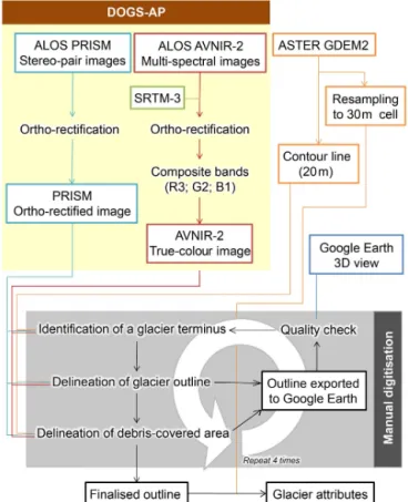
We utilised ALOS satellite imagery. First, we used PRISM-derived stereo-pair panchromatic imagery with a spatial res-olution of 2.5 m, acquired between 2007 and 2011 (Ta-ble S1 in the Supplement), to generate DEMs. The DEMs were then used in conjunction with DSM (digital surface model) and Ortho-image Generation Software for ALOS PRISM (DOGS-AP; Takaku and Tadono, 2009; Fig. 2) to ortho-rectify the original images. This software was devel-oped specifically for generating DEMs and ortho-rectified imagery from PRISM Level 1B1 standard imagery, which supports the rigorous sensor models of PRISM, ALOS orbit data, and ALOS attitude data (Takaku and Tadono, 2009). In this study site, we reported an accuracy of 0.37 m root-mean-square error for the horizontal component in position-ing (Ukita et al., 2011). Because all PRISM images included cloud and seasonal snow cover, we selected the best mul-titemporal PRISM images available for each glacier, typi-cally those collected between October and February. We se-lected 58 PRISM images from the 1364 available (Table S1). Multi-spectral visible and near-infrared imagery, with a spa-tial resolution of 10 m, was acquired via an additional ALOS sensor, the Advanced Visible and Near Infrared Radiome-ter Type 2 (AVNIR-2; Table S2). The AVNIR-2 images ac-quired between 2007 and 2011 were ortho-rectified using the 90 m Shuttle Radar Topography Mission (SRTM3 v3) DEM in DOGS-AP. Composite true-colour images were generated from bands 3, 2, and 1, corresponding to red, green, and blue, respectively.
We used the second version of the Global Digital Elevation Model by ASTER (ASTER GDEM2) to perform glacier de-lineations and spatial analysis. This model was provided by
the Earth Remote Sensing Data Analysis Center, Japan Space Systems, with a cell size of 1 arcsec (∼30 m) and in geo-graphic coordinates covering the global surface (Tachikawa et al., 2011). The absolute length of 1 arcsec varies depending on the latitude, therefore GDEM2 pixels were resampled to 30 m cell size on the Universal Transverse Mercator (UTM) coordinate system zone 46. We chose the ASTER GDEM2 over SRTM3 because the latter exhibited less consistency with Ice, Cloud, and land Elevation Satellite (ICEsat)-derived data in the high mountains of Asia, including a negative bias of −99 m and a large analytical uncertainty. A lower
bias of+40 m was shown by ASTER GDEM2 (Nuimura et
al., 2015).
Precipitation data from the Tropical Rainfall Measur-ing Mission (TRMM) Multi-satellite Precipitation Analy-sis (TMPA) were used to explore the relationship between glacier distribution and climate potential for glacier accu-mulation. These data were generated using a calibration-based sequential scheme that combines precipitation esti-mates from multiple satellites and rain gauge data at a pixel spacing of 0.25◦(∼25 km; Huffman et al., 2007). Yamamoto
et al. (2011) used in situ measurements in the Nepal Hi-malaya to demonstrate that the TMPA data have superior consistency to other precipitation products. Nonetheless, the 0.25◦ spacing means that both sides of a high mountain range are included within a single pixel and, therefore, that stark differences in precipitation (i.e. greater rain/snowfall on the windward, upstream side and less precipitation on the downstream side) are poorly resolved. For this reason, we avoided spatially detailed assessments in favour of provid-ing an overview of the distribution of annual precipitation amounts. A monthly product, TRMM 3B43, was obtained for the period 1998–2014 and averaged to provide mean an-nual precipitation data.
In addition, we calculated the annual flux of solar radiation for each glacier. Intensity of received solar radiation depends primarily on slope inclination and aspect, and these data are provided via spatial analysis of the ASTER GDEM2 for each date and time. Using a basic tool in ArcGIS, solar radiation was estimated from the DEM (30 m cell size) every 0.5 h for each month, and those data were summed to provide an an-nual flux in GJ m−2. This process considers the latitude of the study site homogeneously set at 28◦N, as well as the effects of shading by adjacent mountains, but does not consider ac-tual cloud cover and other meteorological factors. Calculated values are averaged within individual ALOS-derived glacier outlines to produce a single value for each glacier.
2.3 Manual digitisation of glacier outlines
We designed a practical procedure for delineating glaciers and debris-covered areas in PRISM and other satellite im-agery (Fig. 2). Because automatic classification of glacier surfaces from a multispectral image cannot yet be applied to such high-resolution panchromatic imagery (i.e. single-band
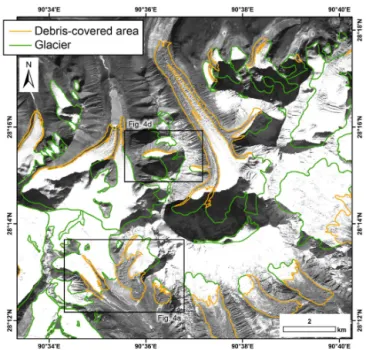
Figure 3.Examples of manually delineated outlines of glaciers and debris-covered areas.
image), time-consuming manual delineation is currently the only way to take advantage of the high-resolution images needed for identifying complex features on glacier surfaces. Additionally, whereas Nagai et al. (2013) delineated out-lines for only debris-covered glaciers, this study makes de-lineations for all glaciers, including debris-free glaciers, and provides attribute information of glaciological parameters for each. Our Bhutanese study follows the definition of a glacier proposed by Global Land Ice Measurements from Space (GLIMS) (Raup and Khalsa, 2007), with the sole ex-ception that we excluded adjacent snow-covered slopes on which glacier flow is not expected (e.g. Figs. 3, 4).
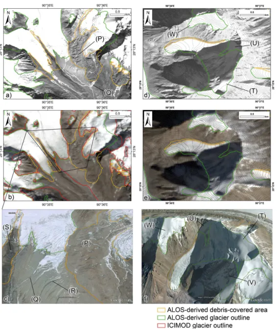
Figure 4. Complex surface features on the termini of debris-covered glaciers in our study site, shown in (a)ALOS PRISM imagery,
(b)Landsat-8 imagery, and(c)Google Earth (location shown in Fig. 3). (P) Small ponds, ice cliffs, and bumpy surface relief, as well as
(Q) traces of water stream, are recognised in(a)and(b), whereas (R) bedrock and moraine surfaces are hard to identify in(b). (S)
Debris-covered ice is partly exposed and identified. Delineation of a glacier with steep surrounding slopes located in our study site, shown in
(d)ALOS PRISM,(e)Landsat 8 imagery, and(f)Google Earth (location shown in Fig. 3). (T) Heavily snow-covered surface, on which
ice flow is expected, is identified as part of the glacier, whereas the regions (U) and (V) are snow-covered areas with poor snow depth for accumulation that are excluded from the glacier because surface features suggest no ice accumulation on these surfaces. The isolated ice mass (W) is included as part of the glacier because its mass probably provides ice to the glacier.
panchromatic imagery. PRISM data were unavailable for 32 glaciers located in the northernmost part of the study site, for which AVNIR-2 imagery alone was used. Delineated out-lines smaller than 0.01 km2in area (n=20, with a total area
of 0.15 km2) were removed to minimise the risk of including snow patches.
Manual delineation of debris-covered areas requires care-ful observation and interpretation of surficial features in
aid-ing the delineation of glacier outlines (e.g. Q in Fig. 4). Boundaries between debris-covered and debris-free ice sur-faces (i.e. the onset of debris cover) can vary among PRISM scenes of different dates owing to snowfall. In such cases, the most expansive debris-covered area was adopted and delineated. Several rock glaciers, flowing masses of boul-ders with less ice content, are identifiable in the study site by their steep front and furrowing and creeping forms in high-resolution satellite imagery. In most cases, they do not have the thermokarst-like features found on a typical covered glacier, though gradual transitions between debris-covered glaciers and rock glaciers can exist. This study does not delineate rock glaciers because they are not defined as a type of glacier (Raup and Khalsa, 2007).
Snow-covered rock walls adjacent to the ice surface were also excluded from our delineations of glacier area (Fig. 4d). First, we focused on the difference in the concentration of contour lines between glacier surfaces and rock walls, the former being relatively gentle compared with the latter. This difference results in relatively sparsely distributed contour lines on the ice surface and more concentrated contour lines on the walls. The contact between the two represents the edge of the glacier, even if it is obscured by snow in the PRISM imagery. Partly snow-covered walls, with exposed and identi-fiable bedrock, were excluded. Careful division was required for those glaciers that are connected to deeply snow-covered rock walls lacking bedrock exposures. Slopes exhibiting un-broken snow cover and that appeared to be thick and sta-ble ice masses, and which suggested regular flow rather than avalanche feeding, were included in glacier outlines (e.g. T in Fig. 4). However, the specific threshold value of a DEM-derived slope gradient was not defined for this delineation since hanging glaciers can have steeper gradients than the surrounding bedrock and must be included.
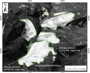
Ice surfaces connected to multiple glacier termini were separated along a hydrological boundary, such as a water-shed or ridge line, by delineating orthogonal lines against GDEM2-derived contour lines (Fig. 5). Unlike the second Chinese Glacier Inventory (CGI2) (Guo et al., 2015), we did not perform automatic watershed separation because we in-tended to compare the results of automatic separation against visual interpretation in complex terrain. Typically, the gen-eration of DEMs for snow-covered surfaces is problematic, as control points can be obscured by snow. However, we did not observe any unnatural contour lines, which hamper manual delineation, at this site. Careful interpretation is re-quired to distinguish connecting glacier termini (Fig. 5). In the case that separation was difficult, they were integrated into a single glacier. Similarly, any detached ice masses lo-cated just above a glacier were included in the delineation if ice redistribution was expected. Shapes for these features are recorded and registered in the inventory as a single row in the attribute table, with the same ID, area, and other variables.
Upon delineation of glacier outlines and debris-covered ar-eas, outlines were corrected by review of exported glacier
Figure 5.Separation of connected glaciers in our study site. Basic separation is performed along ridge lines identified by contour lines. Glacier surfaces with vague termini were not separated.
polygons into Google Earth, which includes high-resolution Quickbird images superimposed upon the SRTM3 topogra-phy (Fig. S1 in the Supplement). Detailed surface features and 3-D visualisation are invaluable for identifying delin-eation errors (e.g. Raup et al., 2014). Whenever a signifi-cant error was identified in cloud-free, high-quality Google Earth imagery, the original outline was corrected manu-ally in ArcGIS (in another screen). Especimanu-ally outlines of north-facing accumulation areas neighbouring steep moun-tain ridges are carefully checked because of mounmoun-tain shad-ows in the PRISM and AVNIR-2 imagery acquired in the winter season. To validate the final corrected version, this manual delineation process was repeated four times. More-over, in order to validate manual delineations based on ALOS imagery, each author independently delineated 10 debris-free glaciers and six debris-covered glaciers, as well as their debris-covered areas. Four outlines were provided for each glacier entity (as well as one debris-covered area) and consis-tencies among them were evaluated using the overlap ratio. 2.4 Glacier attributes
Statistical information for delineated glaciers was calculated by ArcGIS tools and recorded in an attribute table, provided here as supplementary material. A local identification (ID) number was assigned for each glacier polygon. Spatially dis-connected polygons, regarded as one glacier entity according to GLIMS guidelines (e.g. W in Fig. 4), were merged and assigned a single ID. Scene ID and acquisition date for the primary PRISM image and the most appropriate AVNIR-2 image were also noted in the attribute table.
Elevations of maximum, minimum, mean, and median eleva-tion were obtained for individual glaciers using the ASTER GDEM2. Median elevation represents the altitude at which a glacier polygon is separated into upper and lower halves of equal area. This point constitutes an index for denot-ing glacier distribution relative to a balanced-budget equilib-rium line altitude (e.g. Braithwaite and Raper, 2009; Sakai et al., 2015).
We divided the study site into 11 river basins (Fig. 1) that were generated automatically using the ASTER GDEM2 and ArcGIS watershed analysis tools. On the southern flanks, basin names follow those reported by Mool et al. (2001). On the north side of the range, rivers flowing to the Tibetan Plateau were named Nianchu, Langkamu, and Subansiri in reference to the attribute table of the ICIMOD inventory (Ba-jracharya and Shrestha, 2011).
Slope gradients were obtained for each glacier by averag-ing the surface gradients of the ASTER GDEM2 for each glacier. Values for upper and lower halves were calculated separately and divided by the median elevation, and are as-sumed to represent slope gradients for the accumulation and ablation zones, respectively. The glacier aspect was calcu-lated as the mean value of surface aspect on a glacier surface. The aspect value of a GDEM2 pixel (0–360◦) is converted to a unit vector (xaxis for longitudinal range andyaxis for lat-itudinal range). Finally, the averaged unit vector is converted back to an aspect value (0–360◦).
2.5 Other glacier inventories
In the present study site, existing glacier outline data sets are available from GAMDAM, ICIMOD, and RGI, and were ref-erenced onto the Universal Transverse Mercator (UTM) co-ordinate system (zone 46). Contained outlines smaller than 0.01 km2 in area were not analysed in this study to min-imise the risk of including snow patches. We did not include the GLIMS database because the latest version, released on 2 December 2014, includes considerable duplication on the northern side of the range and because no glaciers were de-lineated on the southern side.
Comparison between the GAMDAM and ALOS-derived inventories highlights the differences between the types of satellite imagery used, as similar manual delineations were performed by similar authors. The GAMDAM inventory contains more than 83 000 glaciers distributed throughout the high mountains of Asia (Nuimura et al., 2015), of which we examined those lying within our study site. These glaciers were delineated manually using two Landsat-7 scenes ac-quired on 28 December 2000 and 20 November 2001, along with SRTM-derived contour lines (20 m interval) for glacier separation and differentiation of adjacent headwalls. Delin-eations were then verified via high-resolution Google Earth imagery. While the methods and criteria of the GAMDAM inventory are similar to our own, the ALOS-derived outlines used in this study were delineated solely by the first author,
who did not participate in the Bhutan domain of the GAM-DAM inventory. Therefore, we can evaluate consistency be-tween the ALOS and GAMDAM outlines objectively.
The first ICIMOD glacier inventory, published in 2001, utilised Landsat-5, Indian Remote Sensing (IRS)-1D, and Satellite Pour l’Observation de la Terre (SPOT) imagery ac-quired in the 1990s, in addition to a 1:50 000 scale
to-pographic map depicting glacier distribution in the 1950s (Mool et al., 2001). The latest ICIMOD glacier inventory, published in 2014, includes glacier outlines for the Bhutan Himalaya that were generated using Landsat-5/-7 imagery for the periods 1977–1978, 1990, 2000, and 2010 with semi-automatic classification (Bajracharya et al., 2014a). We utilised the 2010 outlines, in which glacier ice was clas-sified by a threshold of normalised difference snow index (NDSI). Erroneously incorporated shadows, water bodies, vegetation, bare rock, and debris outside of glacier surfaces were removed by multiple filters including the normalised difference vegetation index, a land and water mask, and mean hue with respective threshold values (Bajracharya et al., 2014a). Slopes>60◦and surfaces <4600 m a.s.l. were removed using the SRTM3 DEM. Debris-covered areas in the elevation range 3000–6000 m a.s.l. were extracted from the remaining terrain via the SRTM3-derived slope gradi-ent (<25◦), normalised difference vegetation index, NDSI, and land/water mask. Finally, outlines of debris-covered and debris-free glaciers were superimposed onto high-resolution satellite images in Google Earth and corrected manually (Ba-jracharya et al., 2014a).
2.6 Overlap ratio
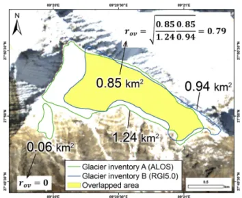
To evaluate the geometric consistency among the multiple in-ventories, we propose an index of overlapping glacier outline between two inventories (rov), which is defined as
rov=
s C
SA C
SB, (1)
whereC is the overlapping area, andSA andSBare the to-tal areas of a glacier polygon in two inventories of A and B, respectively. A higherrovvalue means a larger proportion of the overlapping area is shared by two inventories, and an rov of zero signifies no overlap. For example, outlines from ALOS (1.24 km2) and RGI5.0 (0.94 km2) produce an over-lapped area (0.85 km2), whereas an outline without overlap-ping area causes zero ofrov (Fig. 6). If one polygon in the A inventory is overlapped by several polygons in the B in-ventory, the largestrovis adopted as the ratio of the targeted glacier in the A inventory.
Between two polygons from different inventories for one glacier, relative omission and commission parts are incorpo-rated into the value of overlap ratio. If one polygon (SA) is smaller than another (SB), the shared part (C) is also smaller thanSB, which causes a small value forroveven ifCequals SA. This means that a large area of omission causes small rovvalues. On the other hand, because this is a relative com-parison of two delineated polygons from different sources, absolute omission/commission errors based on actual glacier entities cannot be described. Multiple combinations should be discussed to evaluate consistencies of each delineation. Thus, the overlap ratio enables assessment of the consistency among glacier outlines, including location shifting in various sizes, which would be difficult to perform when using with absolute value of delineated areas.
To assess the consistency between two inventories, the mean value of the overlapping ratio (RAB), in which the A and B inventories are defined as base and target inventories, respectively, is calculated as
RAB= 1
NA X
rov, (2)
whereNAis the number of glaciers in the A inventory. This value can vary according to the number of non-overlapping polygons (rov=0) in the two respective inventories, for ex-ample.
3 Results
3.1 Validation of the ALOS glacier outline
Ten debris-free glaciers, six debris-covered glaciers, and their debris-covered areas were delineated from the ALOS PRISM/AVNIR-2 images by four authors operating indepen-dently. Overlap ratios were calculated for all combinations
Figure 6.Conceptual example of the overlap ratio (rov). The back-ground is an ALOS AVNIR-2 image.
of the four authors (six ways). Mean values and standard deviations of the ratios calculated for the 16 glaciers are summarised against their ALOS-derived sizes (Fig. 7a). All debris-free glaciers give mean values forrovgreater than 0.7, with six exceeding 0.9. Debris-covered glaciers give values greater than 0.5, with larger glaciers giving higher (∼0.8)
values. Similarly, debris-covered areas give higher values with increasing area.
To assess delineation uncertainties quantitatively, we com-pared and analysed the glacier areas of the four interpreters in closer detail. Mean values and standard deviations of the de-lineated area were calculated for each glacier to obtain their respective uncertainty ratios (i.e. standard deviation divided by mean area as a percentage) (Table 1). The uncertainty ratio varies from 1.97 to 48.62 %, with larger values im-plying greater uncertainty. Plotting the ratios against glacier size, uncertainties tend to be smaller for larger glaciers re-gardless of debris cover (Fig. 7b). The highest delineation uncertainty (as much as 50 %) is expected for the small-est (0.01–0.1 km2area) debris-covered glaciers and the low-est (<10 %) for larger (1.0–10 km2), debris-free glaciers. In a case of relatively larger debris-covered glacier (Fig. 7c), uncertainty ratio is indeed smaller (<20 %), however abso-lute area of delineated glacier outlines greatly ranges from 42.51 to 63.78 km2 (Table 1, Fig. 7c). Complicated topog-raphy with shadows and ice distribution at the surrounding steep slopes has the potential to cause large area differences with inconsistent interpretations.
3.2 Statistics of Bhutanese glaciers obtained from the ALOS glacier inventory
debris-Figure 7.Validation of manual glacier delineation using ALOS imagery.(a)Mean values ofrov and their standard deviations, from six
combinations among four outlines, are plotted against glacier area (or debris-covered area).(b)Deviations of glacier delineation in 16
sam-pled glaciers.(c)Debris-covered glaciers and debris-covered areas contain inconsistencies among four interpreters (coloured respectively),
whereas(d)a simple shape of a debris-free glacier exhibits good consistency.(e)A debris-free glacier with steep slopes has inconsistencies
on the higher parts of the outline (region in shadow).
free glaciers (Table 2, Fig. 1). The area of the debris-free glaciers ranges from 0.01 to 5.9 km2 (mean area 0.4 km2), resulting in a total area of 536 km2, whereas that of debris-covered glaciers ranges from 0.06 to 79.6 km2 (mean area 4.3 km2), giving a total area of 951 km2(Fig. 8). The debris-covered area ranges from 0.01 to 21.2 km2, resulting in a
mean area of 1.0 km2. The majority (n=649) of
ALOS-derived glaciers belong to the 0.1–0.5 km2 size category, whereas the greatest number of debris-covered glaciers (n=
debris-Table 1.Delineated glacier area by authors (km2).
Area Interpreter Mean Standard Uncertainty
(km2) deviation ratio (%)
1 2 3 4
Debris-co
v
ered
0.29 0.39 0.12 0.14 0.23 0.11 49
1.08 1.85 1.23 0.78 1.23 0.39 32
6.63 10.57 7.99 9.01 8.55 1.44 17
10.02 12.11 8.77 10.48 10.35 1.20 12
43.75 63.78 50.66 42.51 50.17 8.45 17 (Fig. 7c)
81.47 87.58 80.56 50.57 75.05 14.39 19
Debris-free
0.05 0.05 0.05 0.06 0.05 0.00 7
0.09 0.15 0.07 0.14 0.11 0.03 29
0.09 0.10 0.09 0.12 0.10 0.01 12
0.40 0.66 0.43 0.49 0.50 0.10 20
0.58 0.61 0.60 0.60 0.60 0.01 2
0.97 1.52 1.04 1.07 1.15 0.22 19 (Fig. 7e)
0.98 1.01 0.98 1.07 1.01 0.04 4
1.13 1.18 1.18 1.19 1.17 0.02 2 (Fig. 7d)
3.18 3.65 3.34 3.75 3.48 0.23 7
5.59 7.77 7.38 7.82 7.14 0.91 13
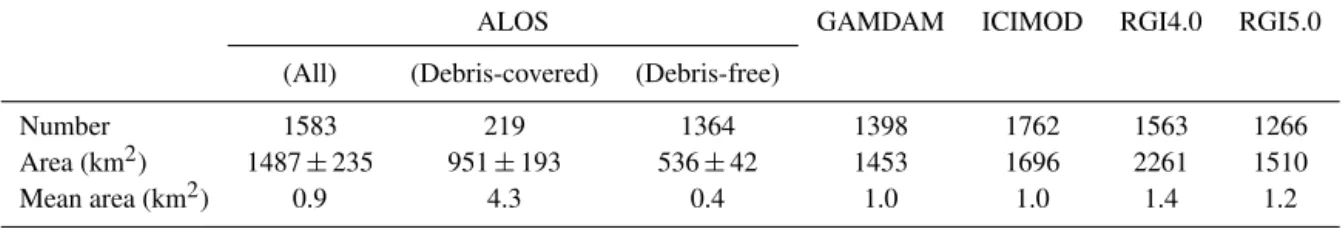
Table 2.Glacier number and area data from the ALOS (all, debris-covered/debris-free), GAMDAM, ICIMOD, RGI4.0, and RGI5.0 inven-tories for the Bhutan Himalaya.
ALOS GAMDAM ICIMOD RGI4.0 RGI5.0
(All) (Debris-covered) (Debris-free)
Number 1583 219 1364 1398 1762 1563 1266
Area (km2) 1487±235 951±193 536±42 1453 1696 2261 1510
Mean area (km2) 0.9 4.3 0.4 1.0 1.0 1.4 1.2
covered glacier (375 km2). In larger size classes, debris-covered glaciers are both more numerous and more extensive than debris-free ice, representing 100 % of glaciers>10 km2 in area.
The anticipated uncertainty ratio for the 16 glaciers (Fig. 7b) was applied to the entire ALOS-derived glacier inventory. Uncertainties for the individual ALOS-derived glacier outlines are calculated by means of the trend lines shown in Fig. 7b. Summation of anticipated uncertainty reaches 235 km2 (16 % of the total glacier area), where debris-covered and debris-free glaciers have anticipated un-certainties of 193 km2 (20 %) and 42 km2 (8 %), respec-tively (Table 2). In addition, they are classified into eight classes of size, where total area uncertainty is divided by total glacier area (Fig. 8c). Debris-covered glaciers in the smallest size class (0.05–0.1 km2) exhibit the largest un-certainty ratio, at 52 %, whereas those in the largest size class (>50 km2) reveal the smallest uncertainty ratio, at 13 %. Similarly, debris-free glaciers exhibit the smaller un-certainty ratio for larger size classes (i.e. 11 % for the 0.01– 0.05 km2class, 6 % for the 5–10 km2class). The area
propor-tion of debris-covered glaciers versus debris-free glaciers is smaller/larger in smaller/larger size classes, with which in-fluencing uncertainty ratio also shifts from∼10 to∼25 %
for larger sizes. Integrating both types of glacier, therefore, the smallest uncertainty ratio is exhibited by the 0.1–0.5 km2 class (10 %). The highest is exhibited by the 5–10 km2class (20 %) with which area proportion of debris-covered versus debris-free glacier is highest (221 to 12 km2) (Fig. 8c). In the size classes larger than 10 km2, the uncertainty ratio is di-rectly controlled by that of debris-covered glaciers without any debris-free glaciers. The maximum uncertain area is ex-hibited by the 1–5 km2 size class (78 km2) with the largest total area of debris-covered/debris-free glaciers.
Figure 8.Cumulative glacier(a)number and(b) area values for
eight size classes.(c)Estimated area of delineation uncertainty ratio
is shown on debris-covered, debris-free, and total glaciers from the ALOS-derived glacier inventory.
Figure 9. Hypsographic curves of glacier surfaces from the ALOS, GAMDAM, ICIMOD, RGI4.0, and RGI5.0 inventories. Also shown are the curves for the debris-covered area, and the debris-covered and debris-free glaciers, extracted from the ALOS inventory.
4600 to 7000 m a.s.l., with a maximum area of 77 km2 at 5400 m a.s.l. Although both covered and debris-free glaciers exhibit maximum areas at approximately the same elevation, the distribution range of the debris-covered glaciers is significantly wider (3500 m) with a larger total area (951 km2 in Table 2) than that of debris-free glaciers (2400 m/536 km2).
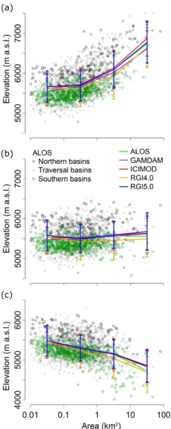
We compared the maximum, median, and minimum ele-vations of individual glaciers with their respective areas on a log scale (Fig. 10). The maximum and minimum eleva-tions tend to be higher and lower, respectively, for larger glaciers, whereas median elevations show neither increas-ing nor decreasincreas-ing trends. To assess elevation distribution in greater detail, we categorised glaciers by location. North-ern basins include Nianchu, Langkamu, and Subansiri, while southern basins include Chamkhar, Mangde, Pho, Mo, Wang, and Amo. Traversal basins include Dangme and Kuri. An ele-vational comparison of glaciers of equal size revealed that the majority of glaciers located in southern basins occur at lower elevations than those in northern basins, while glacier eleva-tion is widely distributed in the traversal basins (Fig. 11).
The spatial distribution of mean annual precipitation amount, obtained from TRMM 3B43 for the period 1998–2014, is shown in Fig. 11. Maximum precipitation (1136 mm) occurred at 27.625◦N, 91.375◦E and minimum precipitation (417 mm) at 28.375◦N, 89.625◦E, resulting in a mean value of 807±202 mm for our study site. Northern
Figure 10.Glacier(a)maximum,(b)median, and(c)minimum el-evations in the ALOS inventory plotted against the log-scaled area. Glaciers are categorised as southern, northern, and traversal basins, as described in Fig. 1. Mean (lines) with standard deviation (vertical bars) of all inventories were calculated in four size classes.
the Tibetan Plateau. In contrast, southern regions experience in excess of 2000 mm precipitation per year, but glaciers do not exist there because the elevation is lower. The main Hi-malayan crest is characterised by west to east (W–E) oriented watersheds, occupied by numerous glaciers, and serves to hinder the northward passage of humid monsoon air masses; yet stark differences in precipitation are not apparent on ei-ther side of the range, as high peaks and valley bottoms are frequently included in the same pixel. Thus, even significant differences in local precipitation are not resolved fully by the 3B43 data.
The median elevations of individual glaciers were over-lain onto a TRMM-derived spatial distribution of mean an-nual precipitation (Fig. 11), revealing a clear north–south contrast (i.e. higher values to the north and lower values to the south). Additionally, the spatial distribution of annual precipitation exhibits a north–south gradient, ranging from 462 to 1040 mm. Statistically, however, significant correla-tion was not observed for each glacier between annual pre-cipitation and median elevation (r <0.1), possibly because most parts of the significant north–south gradient of median elevation are distributed within a small area beyond mountain ranges, which is contained by one grid size of precipitation data (0.25◦).
Mean slope gradients were calculated for both the upper and lower halves of individual ALOS-derived glacier sur-faces, as well as for the entire surface (Fig. 12). The upper (lower) halves are assumed to comprise accumulation (ab-lation) zones. For the upper parts, the mean slope gradients reveal no correlations versus glaciers, whereas those for the lower parts denote negative correlations. This is related to the fact that a larger glacier, in many cases with a debris-covered ablation zone, tends to be developed on valley topography with a gentle slope (e.g. Scherler et al., 2011a). We observed no tendency in slope steepness between the differently cate-gorised basins.
ALOS-derived glacier outlines were classified by aspect (Fig. 13). The number of debris-free glaciers on north-facing slopes is 3 times greater than on south-north-facing slopes, whereas debris-covered glaciers show little or no aspect de-pendency (Fig. 13a). Conversely, the area of the debris-covered glaciers exhibits considerable bias in both north and south basins (Fig. 13b). Mean values of median elevation for the eight aspects were calculated for each river basin (Fig. 14a). The highest ALOS-derived values occur in the Nianchu and Langkamu basins, followed by the Dangme and Kuri basins. Lower median elevations were observed in the southern basins. While south-facing glaciers have the high-est median elevation in the Langkamu, Mo, and Wang river basins, in other regions we found no consistent inclination in the relationship between median elevation and surface as-pect.
Figure 11.Spatial distributions of median elevation for the ALOS-derived glacier outlines, overlain on the spatial distribution of annual precipitation from TRMM 3B43 data (1998–2014).
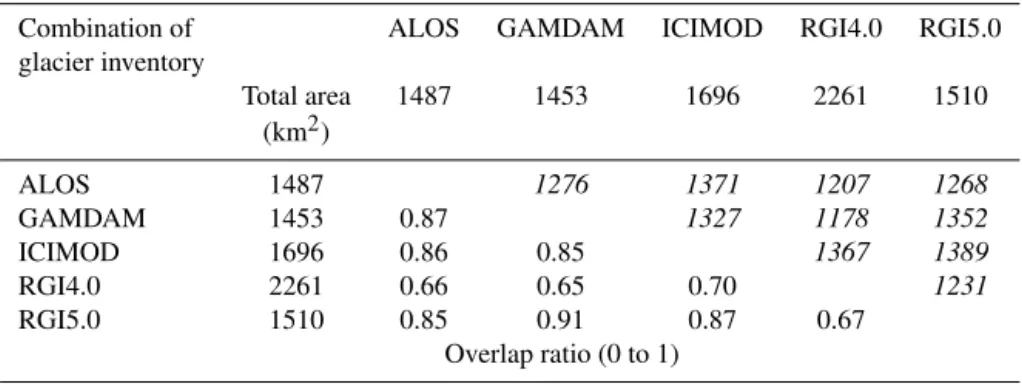
Table 3.Surface area and overlap ratios for the whole glacier surface in the Bhutan Himalaya among the six inventories, in which one
inventory represents one glacier surface. The numbers in italic font denote overlapped area (km2).
Combination of ALOS GAMDAM ICIMOD RGI4.0 RGI5.0
glacier inventory
Total area 1487 1453 1696 2261 1510
(km2)
ALOS 1487 1276 1371 1207 1268
GAMDAM 1453 0.87 1327 1178 1352
ICIMOD 1696 0.86 0.85 1367 1389
RGI4.0 2261 0.66 0.65 0.70 1231
RGI5.0 1510 0.85 0.91 0.87 0.67
Overlap ratio (0 to 1)
ASTER GDEM2 with 30 m cell size. Although the influ-ence of surrounding topography was considered, the effects of cloud cover were impossible to determine. Results range from 4.0 to 9.6 GJ m−2. The mean annual radiation flux for each glacier was then calculated and plotted against aspect. Our data show that north-facing glaciers received less radi-ation than south-facing glaciers. Additionally, the radiradi-ation flux over south-facing glaciers is apparently independent of slope gradient.
3.3 Consistency among glacier inventories
We first calculated overlap ratios for each of the five glacier inventories. The glacier surface was integrated such that one glacier area was determined for each inventory (Ta-ble 3). High ratios of >0.85 were obtained for the ALOS,
GAMDAM, ICIMOD, and RGI5.0 inventories, whereas the RGI4.0 inventory gave low ratios of <0.75. Total overlap ratios for RGI4.0/5.0 suggest that while the RGI4.0 inven-tory contains larger areas that do not overlap with the other inventories, this situation has been improved in the RGI5.0 version.
Second, the number of glaciers is cumulated from those with a lower overlap ratio and cumulative curves for every combination of the inventories and is illustrated in Fig. 15. In comparison to the ALOS-derived inventory, the GAMDAM, ICIMOD, and RGI5.0 inventories reveal similar curves that increase towards larger rov values (∼0.7), indicating that
Figure 12.Slope gradients of the(a)upper half,(b)entire surface,
and (c)lower half of ALOS-derived glacier outlines, categorised
as northern/southern/traversal basins as shown in Fig. 1. Calculated mean values and standard deviations for four size classes are shown along with those of other inventories.
on which the number of glaciers with lowrov (0.5) reaches 1000. Consequently, mean values for overlap ratios (Rbasetarget) are highest for the ALOS–ICIMOD combination (0.63) and lowest for the ALOS–RGI4.0 combination (0.35). Values for the ALOS–RGI combination show a marked improvement from RGI4.0 (0.35) to RGI5.0 (0.56). In analysing other combinations (Fig. 15b–e), the RGI4.0 inventory exhibits uniformly poor overlap with the other inventories.
Figure 13.Cumulative glacier(a)number and(b)area of ALOS-derived glacier outlines, classified by aspect. Also plotted are total glacier number and area data from other inventories.
Figure 16a depicts area differences of the four inventories against our ALOS-derived inventory, in which the area differ-ence among glacier outlines ranges from 0.1 to 10 times. The RGI4.0 in particular includes numerous glaciers for which the area exceeded 10 times that of the ALOS-derived inven-tory. Figure 16b shows variations in the standard deviation of area difference (ratios in Fig. 16a) calculated within six size classes. Smaller glaciers exhibit larger standard devia-tions, whereas larger glaciers show lower values. While each inventory shows this trend, the greatest standard deviations occur in the RGI4.0 inventory.
Figure 14. (a) Median elevations in 9 of 11 river basins (Fig. 1)
are plotted along eight aspects.(b)Estimated mean values of
an-nual solar radiation for respective ALOS-derived glacier outlines, for which glaciers are grouped into three classes based on their mean slope gradients.
whereas the RGI4.0 exhibits the greatest, at 2261 km2 (Ta-ble 2). We categorised these results into eight size classes (Fig. 8). The total glacier number and area differed widely among the inventories. However, in each, the majority of glaciers fall between 0.1 and 0.5 km2 total glacier number (Fig. 8a). Similarly, the greatest total area lies in the 1–5 km2 size class for each inventory, although the overall difference between RGI4.0 and GAMDAM reaches ∼300 km3 in the
size class (Fig. 8b).
We also compared the hypsometric curves of glacier out-lines (Fig. 9). The maximum area of 187 km2 occurs at 5600±50 m elevation in the RGI4.0. The other inventories
show a similar pattern. The ALOS, GAMDAM, ICIMOD,
Figure 15.Cumulative glacier numbers against overlap ratios (rov) for the six glacier inventories covering the Bhutan Himalaya.
Glacier number increases from the lowerrov to the higher rov,
where a constant increase means a large number of low-rovoutlines,
and a later high rate of increase means a large number of high-rov
outlines. Meanrovvalues for each combination are denoted in the
panels.
and RGI5.0 outlines are located within the 4000–7500 m el-evation range, whereas the lowermost outlines in the RGI4.0 occur at 2600 m a.s.l.
Figure 16. (a)Area difference between the ALOS-derived glacier
inventory and other inventories.(b)Standard deviations of area
dif-ference are summarised in seven area classes.
on larger glaciers. Finally, we compared ALOS-derived total glacier numbers and areas in the eight aspect groups with the other inventories (Fig. 13a, b). Although we observed signifi-cant differences among the values, all five inventories exhibit similar trends.
4 Discussion
Our results suggest that although existing glacier inventories give different values for number, area, and topographic vari-ables, they reveal similar statistical and topographical ten-dencies. The geometric differences in glacier outlines can be quantified using the overlap ratio, which enables relative evaluation among the inventories. In this section, we discuss glacier distributions in the Bhutan Himalaya obtained via the various inventories, examine the causes and effects of outline diversity using examples, and provide suggestions for mak-ing glacier delineations in areas of complex topography. 4.1 Glacier distribution in the Bhutan Himalaya Each inventory indicates that glaciers with areas of 1–5 km2 occupy the largest area, while those of 0.1–0.5 km2 consti-tute the majority of glaciers by number (Fig. 8). Globally, the RGI5.0 suggests that this pattern is similar throughout the low–mid-latitudes, with the exception of the European Alps (i.e. a large number of small glaciers which do not affect areal proportion), whereas high-latitude regions are dominated by
larger glaciers (Fig. S3). In the Bhutan Himalaya, glaciers exhibit a size distribution typical of low-latitude regions.
In this region, we observed that glaciers in southern basins have lower maximum, median, and minimum elevations than those in northern basins (Figs. 10, 11). Also, we note that peak elevations are lower in southern than in northern basins (Fig. 9b in Nagai et al., 2013). Thus, we consider this to-pographic contrast to be a fundamental factor influencing the differences in maximum elevation between northern and southern basins (Fig. 10a). The north–south gradients in median elevation and precipitation in Bhutan show reason-able agreement, whereas north–south air temperature gradi-ents are relatively minor due to the small latitudinal range (<170 km) (Fig. 11). Therefore, we do not correlate the dis-tribution of median elevations with glacier size, aspect, or de-bris cover, but to basin location, over which precipitation val-ues differ significantly (Figs. 10b, 11, 14a) as found for the whole glaciers in high-mountain Asia (Sakai et al., 2015) and some glaciers chosen globally (Ohmura et al., 1992). Combi-nations of topography and precipitation may result in lower minimum elevations on southern glaciers, for which rapid re-treat has been reported, and vice versa (Karma et al., 2003; Bajracharya et al., 2014a).
ArcGIS-based calculations of annual solar radiation give values of∼9 GJ m−2for south-facing glaciers regardless of
surface gradient, whereas north-facing glaciers experience values of∼8 GJ m−2 for gentle slopes and 5.5 GJ m−2 for
steeper slopes (Fig. 14b). North-facing glaciers are more nu-merous than south-facing glaciers; this suggests a negative impact of solar radiation on small, debris-free glaciers on south-facing slopes. In contrast, large debris-covered glaciers occur on both southerly and northerly aspects (Figs. 1, 13b). The west to east orientation of the Himalayan range provides extensive north- and south-facing slopes (Fig. 1) favourable for the development of large valley glaciers. Potentially, de-bris cover is supplied to south- and north-flowing glaciers, al-though its intensity is greater on the south-facing slopes (Na-gai et al., 2013). Total glacier area is dominated by debris-covered glaciers and is rather concentrated in the two aspects of the south and north, where the Himalayan main range forms larger valleys to develop large glaciers (Fig. 13).
the south side is the only factor for the situation that the num-ber of glaciers is smaller in the south-facing slopes, although it is a reasonable situation for the global trend that south-facing glaciers have higher elevation distribution than north-facing glaciers (Evans and Cox, 2005).
4.2 Inconsistency in glacier identification
Identification of glacier termini affects the consistency among glacier inventories. The largest discrepancy in the number of non-overlapping glaciers (n=471) occurs
be-tween the RGI4.0 and GAMDAM inventory, whereas the smallest (n=34) is found between the RGI5.0 and
GAM-DAM inventory (Fig. 15). In some cases, small glacier-like polygons larger than 0.01 km2 were found where no glaciers exist (Fig. 17a). Since glaciers are unlikely to dis-appear from one inventory to the next, we suggest that tem-porary snow cover is the main reason for this variability and, thus, that multiple images acquired on different dates should be checked. Additionally, snow-covered bedrock sur-faces can present a similar appearance to glacier ice (e.g. Fig. 17b). However, while details of surface roughness in high-resolution Google Earth imagery suggest that these are not ice surfaces, such identification is not possible using the coarse resolution of Landsat-5/-7 imagery (30 and 15 m, re-spectively).
4.3 Inconsistency in glacier distribution
The entire RGI4.0 glacier surface overlaps poorly with those of other inventories (Table 3). Specifically, while the eleva-tion of maximum glacier area lies around 5400 m a.s.l., sim-ilar to other inventories (Fig. 9), minimum glacier elevation in the RGI4.0 is considerably lower at 3000 m a.s.l. Individ-ual glacier outlines in the RGI4.0 also overlap poorly with those in the other target inventories, for which mean val-ues are no greater than 0.35 (Fig. 15d). We found signifi-cant distortion in RGI4.0 outlines when compared with other data sets (Fig. 18), which implies inaccurate cartography and low-quality georeferencing of the original topographic maps as well as a poor condition of the original imagery. This is one possible reason for the uniquely larger glacier area reaching 300 km3larger than that of the GAMDAM inven-tory (Fig. 8b). In contrast, RGI5.0 does not exhibit these in-consistencies, nor do the ICIMOD, GAMDAM, and ALOS-derived inventories, all of which contain large numbers of well-overlapped glacier outlines with values>0.5 (Fig. 15). The ICIMOD inventory was generated using semi-automatic processes, whereas GAMDAM and ALOS-derived outlines were generated via manual delineation. In all cases, the use of Google Earth imagery for manual correction is likely to result in outlines of similar quality. The RGI5.0 contains GAMDAM and CGI2 outlines for southern and northern sides, respectively. Figure 15e shows that the RGI5.0 com-prises a large number of delineations that are highly
consis-Figure 17. (a)Glacier outlines in part of our study site. Some out-lines are delineated only in the (P) ICICMOD, (Q) RGI4.0, and (R)
GAMDAM inventories.(b)A close-up image from Google Earth
suggests that no glacier exists on the (S) snow-covered hill slope
(location shown in box ina). (T) We found differences among the
inventories in their separation of surrounding steep slopes.
tent with GAMDAM data, of which 344 outlines of 1266 ex-hibit a perfect match. Importing GAMDAM outlines to the RGI5.0 inventory thus contributes to the consistency with ICIMOD and ALOS-derived inventories (Fig. 15d, e).
Excessive under- or overestimation of individual glacier areas produced results that range between factors>0.1 and 10 of the ALOS-derived outlines, although the majority of re-sults plot along the one-time line (Fig. 16a). This large differ-ence might be due to the number of glaciers identified from one connecting glacier surface, rather than inaccurate de-lineation or poor georeferencing. While automatic GIS (ge-ographic information system)-based separation of glaciers along ridge lines is necessary to resolve this issue, a remain-ing issue is indistinct glacier termini, which can reduce the consistency of glacier counting (Fig. 5).
Figure 18.Glacier outlines containing significant distortion in the RGI4.0. These have been improved for the RGI5.0 and are now consistent with other inventories.
also affect interpretation of retreat rates for debris-covered glaciers (e.g. Fig. 4b). High-resolution Google Earth satellite imagery reveals numerous ice cliffs on a debris-covered area, suggesting a hidden ice body. Such details are difficult to identify in 30 m resolution Landsat imagery. Detailed visual inspection and manual correction with high-resolution satel-lite images is thus needed, particularly for smaller debris-covered glaciers, which, as described above, exhibit greater inconsistency in manual delineation than larger glaciers do (Fig. 7b).
Steep slopes surrounding the accumulation zone are ex-cluded by ALOS-derived, GAMDAM, and ICIMOD inven-tories, but are included in the RGI4.0 and CGI2. Such head-walls constitute an additional source of glacier nourishment via avalanching (e.g. Benn and Lehmkuhl, 2000; Scherler et al., 2011a; Hewitt, 2011), which must be considered in stud-ies of glacier mass balance and runoff in high relief regions. For example, glacier nourishment from surrounding slopes is especially relevant to the behaviour of Karakoram-type (i.e. Turkistan and Mustagh glaciers) (Hewitt, 2011). In contrast, headwall areas should be avoided when monitoring changes in glacier mass. Thus, the choice of inventory must be based on the purpose of study.
Finally, despite following the same definition of a glacier, differences in interpretation among investigators can result in considerable variability in glacier outlines where steep snow-covered slopes occur immediately adjacent to the glacier (Fig. 7c, e). This factor should be considered during the manual-editing process of automatic delineation by making a comparison with Google Earth imagery. Nonetheless,
con-tinual updating of satellite imagery, temporally variable snow cover, and coarse resolution of images preclude straightfor-ward glacier mapping.
5 Conclusion
surface gradient (Fig. 14) to their respective horizontal ar-eas, and aspect distribution (Fig. 13). Although in situ mea-surements are difficult for the majority of glaciers in high mountain regions, digitised glacier outlines can be validated by comparing those from different sources.
The selection of a specific inventory depends on the pur-pose of an application. While any of them is appropriate when overview information only is required, the correct data set needs to be selected carefully if specific glaciological variables are of interest and individual glaciers are to be anal-ysed. For example, glacier area can vary significantly ow-ing to difficulties in the interpretation of debris-covered areas (Fig. 4) or the separation of individual glaciers (Fig. 5).
The Supplement related to this article is available online at doi:10.5194/tc-10-65-2016-supplement.
Acknowledgements. We thank the editor, T. Bolch, and the reviewers, F. Paul, A. Racoviteanu, M. Pelto, and an anonymous reviewer for their patient handling of this paper and invaluable suggestions. The ALOS data used in this study were provided by the “Study on Glacial Lake Outburst Floods in the Bhutan Hi-malayas” project, conducted as part of the Science and Technology Research Partnership for Sustainable Development (SATREPS), and supported by the Japan Science and Technology Agency (JST) and the Japan International Cooperation Agency (JICA). Support was also provided by the Funding Program for Next Generation World-Leading Researchers (NEXT).
Edited by: T. Bolch
References
Bajracharya, S. R. and Shrestha, B.: The status of glaciers in the Hindu Kush-Himalayan region, International Centre for Inte-grated Mountain Development (ICIMOD), Kathmandu, Nepal, 140 pp., 2011.
Bajracharya, S. R., Maharjan, S. B., and Shrestha, F.: The sta-tus and decadal change of glaciers in Bhutan from the 1980s to 2010 based on satellite data, Ann. Glaciol., 55, 159–166, doi:10.3189/2014AoG66A125, 2014a.
Bajracharya, S. R., Maharjan, S. B., Shrestha, F., Bajracharya, O. R., and Baidya, S.: Glacier status in Nepal and decadal change from 1980 to 2010 based on Landsat data, International Centre for Integrated Mountain Development (ICIMOD), Kathmandu, Nepal, 88 pp., 2014b.
Benn, I. D. and Lehmkuhl, F.: Mass balance and equilibrium-line al-titudes of glaciers in high-mountain environments, Quatern. Int., 65/66, 15–29, 2000.
Bhatt, B. C. and Nakamura, K.: Characteristics of monsoon rainfall around the Himalayas revealed by TRMM precipitation radar, Mon. Weather Rev., 133, 149–165, doi:10.1175/MWR-2846.1, 2005.
Bolch, T., Buchroithner, M., Pieczonka, T., and Kunert, A.: Plani-metric and voluPlani-metric glacier changes in the Khumbu Himal, Nepal, since 1962 using Corona, Landsat TM and ASTER data, J. Glaciol., 54, 592–600, doi:10.3189/002214308786570782, 2008.
Bolch, T., Menounos, B., and Wheate, R.: Landsat-based inventory of glaciers in western Canada, 1985–2005, Remote Sens. Envi-ron., 114, 127–137, doi:10.1016/j.rse.2009.08.015, 2010. Bolch, T., Kulkarni, A., Kääb, A., Huggel, C., Paul, F., Cogley, J. G.,
Frey, H., Kargel, J. S., Fujita, K., Scheel, M., Bajracharya, S., and Stoffel, M.: The state and fate of Himalayan glaciers, Science, 336, 310–314, doi:10.1126/science.1215828, 2012.
Bookhagen, B. and Burbank, D. W.: Topography, relief, and TRMM-derived rainfall variations along the Himalaya, Geophys. Res. Lett., 33, L08405, doi:10.1029/2006GL026037, 2006. Braithwaite, R. J. and Raper, S. C. B.: Estimating equilibrium-line
altitude (ELA) from glacier inventory data, Ann. Glaciol., 50, 127–132, doi:10.3189/172756410790595930, 2009.
Cogley, J. G.: Climate science: Himalayan glaciers in the balance, Nature, 488, 468–469, doi:10.1038/488468a, 2012.
Cogley, J. G.: Glacier shrinkage across High Mountain Asia, Ann. Glaciol., 57, 41–49, doi:10.3189/2016AoG71A040, 2016. Evans, I. S. and Cox, N. J.: Global variations of
lo-cal asymmetry in glacier altitude: separation of north– south and east–west components, J. Glaciol., 51, 469–482, doi:10.3189/172756505781829205, 2005.
Fujita, K. and Nuimura, T.: Spatially heterogeneous wastage of Hi-malayan glaciers, P. Natl. Acad. Sci. USA, 108, 14011–14014, doi:10.1073/pnas.1106242108, 2011.
Gardelle, J., Arnaud, Y., and Berthier, E.: Contrasted evolution of glacial lakes along the Hindu Kush Himalaya mountain range between 1990 and 2009, Global Planet. Change, 75, 47–55, doi:10.1016/j.gloplacha.2010.10.003, 2011.
Gardelle, J., Berthier, E., Arnaud, Y., and Kääb, A.: Region-wide glacier mass balances over the Pamir-Karakoram-Himalaya dur-ing 1999–2011, The Cryosphere, 7, 1263–1286, doi:10.5194/tc-7-1263-2013, 2013.
Gardner, A., Moholdt, G., Cogley, J. G., Wouters, B., Arendt, A., Wahr, J., Berthier, E., Hock, R., Pfeffer, W. T., Kaser G., Ligten-berg, S. R. M., Bolch, T., Martin, J., Sharp, M. J., Hagen, J. O., van den Broeke, M. R., and Paul, F.: A Reconciled Estimate of Glacier Contributions to Sea Level Rise: 2003 to 2009, Science, 340, 852–857, doi:10.1126/science.1234532, 2013.
Guo, W., Liu, S., Xu, J., Wu, L., Shangguan, D., Yao, X., Wei, J., Bao, W., Yu, P., Liu, Q., and Jiang, Z.: The second Chinese glacier inventory: data, methods and results, J. Glaciol., 61, 357– 371, doi:10.3189/2015JoG14J209, 2015.
Hewitt, K.: Glacier change, concentration, and elevation effects in the Karakoram Himalaya, Upper Indus Basin, Mt. Res. Dev., 31, 188–200, 2011.
Houze, R. A., Wilton, D. C., and Smull, B. F.: Monsoon con-vection in the Himalayan region as seen by the TRMM Pre-cipitation Radar, Q. J. Roy. Meteor. Soc., 133, 1389–1411, doi:10.1002/qj.106, 2007.
Huss, M. and Farinotti, D.: Distributed ice thickness and volume of all glaciers around the globe, J. Geophys. Res., 117, F04010, doi:10.1029/2012JF002523, 2012.
Immerzeel, W. W., Van Beek, L. P., and Bierkens, M. F.: Climate change will affect the Asian water towers, Science, 328, 1382– 1385, doi:10.1126/science.1183188, 2010.
Kääb, A.: Combination of SRTM3 and repeat ASTER
data for deriving alpine glacier flow velocities in the Bhutan Himalaya, Remote Sens. Environ., 94, 463–474, doi:10.1016/j.rse.2004.11.003, 2005.
Kääb, A., Berthier, E., Nuth, C., Gardelle, J., and Arnaud, Y.: Contrasting patterns of early twenty-first-century glacier mass change in the Himalayas, Nature, 488, 495–498, doi:10.1038/nature11324, 2012.
Karma, Y. A., Naito, N., Iwata, S., and Yabuki, H.: Glacier distribu-tion in the Himalayas and glacier shrinkage from 1963 to 1993 in the Bhutan Himalayas, Bulletin of Glaciological Research, 20, 29–40, 2003.
Kaser, G., Großhauser, M., and Marzeion, B.: Contribution potential of glaciers to water availability in different cli-mate regimes, P. Natl. Acad. Sci. USA, 107, 20223–20227, doi:10.1073/pnas.1008162107, 2010.
Kienholz, C., Herreid, S., Rich, J., Arendt, A., Hock, R., and Burgess, E.: Derivation and analysis of a complete modern-date glacier inventory for Alaska and northwest Canada, J. Glaciol., 61, 403–420, doi:10.3189/2015JoG14J230, 2015.
Marzeion, B., Jarosch, A. H., and Hofer, M.: Past and future sea-level change from the surface mass balance of glaciers, The Cryosphere, 6, 1295–1322, doi:10.5194/tc-6-1295-2012, 2012. Mool, P. K., Wangda, D., Bajracharya, S. R., Kunzang, K.,
Gu-rung, D. R., and Joshi, S. P.: Inventory of Glaciers, Glacial Lakes and Glacial Lake Outburst Floods, Bhutan, International Centre for Integrated Mountain Development (ICIMOD), Kathmandu, Nepal, 227 pp., 2001.
Nagai, H., Fujita, K., Nuimura, T., and Sakai, A.: Southwest-facing slopes control the formation of debris-covered glaciers in the Bhutan Himalaya, Cryosphere, 7, 1303–1314, doi:10.5194/tc-7-1303-2013, 2013.
Narama, C., Kääb, A., Duishonakunov, M., and Abdrakhmatov, K.: Spatial variability of recent glacier area changes in the Tien
Shan Mountains, Central Asia, using Corona (∼1970),
Land-sat (∼2000), and ALOS (∼2007) satellite data, Global Planet.
Change, 71, 42–54, doi:10.1016/j.gloplacha.2009.08.002, 2010. Nuimura, T., Sakai, A., Taniguchi, K., Nagai, H., Lamsal, D., Tsutaki, S., Kozawa, A., Hoshina, Y., Takenaka, S., Omiya, S., Tsunematsu, K., Tshering, P., and Fujita, K.: The GAM-DAM glacier inventory: a quality-controlled inventory of Asian glaciers, The Cryosphere, 9, 849–864, doi:10.5194/tc-9-849-2015, 2015.
Ohmura, A., Kasser, P., and Funk, M.: Climate at the equilibrium line of glaciers, J. Glaciol., 38, 397–411, 1992.
Paul, F. and Andreassen, L. M.: A new glacier inventory for
the Svartisen region, Norway, from Landsat ETM+ data:
challenges and change assessment, J. Glaciol., 55, 607–618, doi:10.3189/002214309789471003, 2009.
Paul, F., Huggel, C., and Kääb, A.: Combining satellite multi-spectral image data and a digital elevation model for mapping debris-covered glaciers, Remote Sens. Environ., 89, 510–518, doi:10.1016/j.rse.2003.11.007, 2004.
Paul, F., Frey, H., and Le Bris, R.: A new glacier inven-tory for the European Alps from Landsat TM scenes of 2003: challenges and results. Ann. Glaciol., 52, 144–152, doi:10.3189/172756411799096295, 2011.
Paul, F., Barrand, N. E., Baumann, S., Berthier, E., Bolch, T., Casey, K., Frey, H., Joshi, S. P., Konovalov, V., Le Bris, R., Mölg, N., Nosenko, G., Nuth, C., Pope, A., Racoviteanu, A., Rastner, P., Raup, B., Scharrer, K., Steffen, S., and Winsvold, S.: On the accuracy of glacier outlines derived from remote-sensing data, Ann. Glaciol., 54, 171–182, doi:10.3189/2013AoG63A296, 2013.
Pfeffer, W. T., Arendt, A. A., Bliss, A., Bolch, T., Cogley, J. G., Gardner, A. S., Hagen, J., Hock, R., Kaser, G., Kienholz, C., Miles, E. S., Moholdt, G., Mölg, N., Paul, F., Radic, V., Rast-ner, P., Raup, B. H., Rich, J., Sharp, M. J., and the Ran-dolph Consortium: The RanRan-dolph Glacier Inventory: a glob-ally complete inventory of glaciers, J. Glaciol., 60, 537–552, doi:10.3189/2014JoG13J176, 2014.
Racoviteanu, A. E., Williams, M. W., and Barry, R. G.: Optical Re-mote Sensing of Glacier Characteristics: A Review with Focus on the Himalaya, Sensors, 8, 3355–3383, doi:10.3390/s8053355, 2008.
Radi´c, V. and Hock, R.: Regionally differentiated contribution of mountain glaciers and ice caps to future sea-level rise, Nat. Geosci., 4, 91–94, doi:10.1038/ngeo1052, 2011.
Radi´c, V., Bliss, A., Beedlow, A. C., Hock, R., Miles, E., and Cogley, J. G.: Regional and global projections of twenty-first century glacier mass changes in response to climate scenar-ios from global climate models, Clim. Dynam., 42, 37–58, doi:10.1007/s00382-013-1719-7, 2014.
Raup, B. and Khalsa, S. J. S.: GLIMS analysis tutorial. Boulder, CO, University of Colorado, National Snow and Ice Data Center, available at: http://www.glims.org/MapsAndDocs/guides.html, last access: 1 December 2015, 2007.
Raup, B. H., Khalsa, S. J. S., Armstrong, R. L., Sneed, W. A., Hamilton, G. S., Paul, F., Cawkwell, F., Beedle, M. J., Menounos, B. P., Wheate, R. D., Rott, H., Shiyin, L., Xin, Li., Donghui, S., Guodong, C., Kargel, J. S., Larsen, C. F., Molnia, B. F., Kin-caid, J. L., Klein, A., and Konovalov, V.: Quality in the GLIMS glacier database, in: Global Land Ice Measurements from Space, Springer Berlin Heidelberg, 163–182, doi:10.1007/978-3-540-79818-7_7, 2014.
Richardson, S. D. and Reynolds, J. M.: An overview of glacial hazards in the Himalayas, Quatern. Int., 65, 31–47, doi:10.1016/S1040-6182(99)00035-X, 2000.
Sakai, A., Nuimura, T., Fujita, K., Takenaka, S., Nagai, H., and Lamsal, D.: Climate regime of Asian glaciers revealed by GAMDAM glacier inventory, The Cryosphere, 9, 865–880, doi:10.5194/tc-9-865-2015, 2015.
Scherler, D., Bookhagen, B., and Strecker, M. R.: Hillslope– glacier coupling: The interplay of topography and glacial dynamics in High Asia, J. Geophys. Res., 116, F02019, doi:10.1029/2010JF001751, 2011a.
Shi, Y., Lium, C., and Kang, E.: The Glacier Inventory of China, Ann. Glaciol., 50, 1–4, doi:10.3189/172756410790595831, 2009.
Tachikawa, T., Hato, M., Kaku, M., and Iwasaki, A.: The character-istics of ASTER GDEM version 2, Proc. IGARSS 2011 Sympo-sium, Vancouver, Canada, 24–29 July 2011, 3657–3660, 2011. Takaku, J. and Tadono T.: PRISM On-Orbit geometric calibration
and DSM performance, IEEE T. Geosci. Remote, 47, 4060– 4073, doi:10.1109/TGRS.2009.2021649, 2009.
Ukita, J., Narama, C., Tadono, T., Yamanokuchi, T., Tomiyama, N., Kawamoto, S., Abe, C., Uda, T., Yabuki, H., Fujita, K., and Nishimura, K.: Glacial lake inventory of Bhutan using ALOS data: methods and preliminary results, Ann. Glaciol, 52, 65–71, doi:10.3189/172756411797252293, 2011.
Vaughan, D. G., Comiso, J. C., Allison, I., Carrasco, J., Kaser, G., Kwok, R., Mote, P., Murray, T., Paul, F., Ren, J., Rig-not, E., Solomina, O., Steffen, K., and Zhang, T.: Observa-tions: Cryosphere, in: Climate Change 2013: The Physical Sci-ence Basis. Contribution of Working Group I to the Fifth As-sessment Report of the Intergovernmental Panel on Climate Change, edited by: Stocker, T. F., Qin, D., Plattner, G. K., Tignor, M., Allen, S. K., Boschung, J., Nauels, A., Xia, Y., Bex, V., and Midgley, P. M., Cambridge University Press, Cam-bridge, United Kingdom, and New York, N.Y., USA, 317–382, doi:10.1017/CBO9781107415324.012, 2013.
Yamamoto, M. K., Ueno, K., and Nakamura, K.: Comparison of satellite precipitation products with rain gauge data for the Khumbu region, Nepal Himalaya, J. Meteorol. Soc. Jpn., 89, 597–610, doi:10.2151/jmsj.2011-601, 2011.