www.atmos-chem-phys.net/17/935/2017/ doi:10.5194/acp-17-935-2017
© Author(s) 2017. CC Attribution 3.0 License.
MIX: a mosaic Asian anthropogenic emission inventory under the
international collaboration framework of the MICS-Asia and HTAP
Meng Li1,2, Qiang Zhang1,12, Jun-ichi Kurokawa3, Jung-Hun Woo4, Kebin He2,11,12, Zifeng Lu5, Toshimasa Ohara6, Yu Song7, David G. Streets5, Gregory R. Carmichael8, Yafang Cheng9, Chaopeng Hong1,2, Hong Huo10,
Xujia Jiang1,2, Sicong Kang2, Fei Liu2, Hang Su9, and Bo Zheng2
1Ministry of Education Key Laboratory for Earth System Modeling, Department of Earth System Science, Tsinghua University, Beijing, China
2State Key Joint Laboratory of Environment Simulation and Pollution Control, School of Environment, Tsinghua University, Beijing, China
3Asia Center for Air Pollution Research, 1182 Sowa, Nishi-ku, Niigata, Niigata, 950-2144, Japan 4Department of Advanced Technology Fusion, Konkuk University, Seoul, Korea
5Energy Systems Division, Argonne National Laboratory, Argonne, IL, USA
6National Institute for Environmental Studies, 16-2 Onogawa, Tsukuba, Ibaraki, 305-8506, Japan 7State Key Joint Laboratory of Environmental Simulation and Pollution Control, Department of Environmental Science, Peking University, Beijing, China
8Center for Global and Regional Environmental Research, University of Iowa, Iowa City, IA 52242, USA
9Multiphase Chemistry Department, Max Planck Institute for Chemistry, Mainz, Germany 10Institute of Energy, Environment and Economy, Tsinghua University, Beijing, China
11State Environmental Protection Key Laboratory of Sources and Control of Air Pollution Complex, Beijing, China
12Collaborative Innovation Center for Regional Environmental Quality, Beijing, China
Correspondence to:Qiang Zhang ([email protected])
Received: 23 November 2015 – Published in Atmos. Chem. Phys. Discuss.: 10 December 2015 Revised: 9 November 2016 – Accepted: 5 December 2016 – Published: 20 January 2017
Abstract. The MIX inventory is developed for the years 2008 and 2010 to support the Model Inter-Comparison Study for Asia (MICS-Asia) and the Task Force on Hemi-spheric Transport of Air Pollution (TF HTAP) by a mosaic of up-to-date regional emission inventories. Emissions are esti-mated for all major anthropogenic sources in 29 countries and regions in Asia. We conducted detailed comparisons of different regional emission inventories and incorporated the best available ones for each region into the mosaic inven-tory at a uniform spatial and temporal resolution. Emissions are aggregated to five anthropogenic sectors: power, indus-try, residential, transportation, and agriculture. We estimate the total Asian emissions of 10 species in 2010 as follows: 51.3 Tg SO2, 52.1 Tg NOx, 336.6 Tg CO, 67.0 Tg NMVOC (non-methane volatile organic compounds), 28.8 Tg NH3,
1 Introduction
The Model Inter-Comparison Study for Asia (MICS-Asia) project is currently in phase III. During the previous two phases, studies have been focused on long-range transport and deposition of pollutants, global inflow of pollutants to Asia, model sensitivities to aerosol parameterization, and emissions over Asia (Carmichael et al., 2002, 2008; Han et al., 2008; Hayami et al., 2008; Holloway et al., 2008; Wang et al., 2008). MICS-Asia Phase III aims to conduct further inter-comparisons of atmospheric modeling for Asia and analyze the disagreement of model output and relative uncertainties. In this regard, common meteorological fields, emission data, and boundary conditions should be used. One of the key tasks in MICS-Asia Phase III is to develop a reliable Asian emis-sion inventory as common input for model intercomparisons through integration of state-of-the-art knowledge on Asian emissions.
A reasonable understanding of anthropogenic emissions is essential for atmospheric chemistry and climate research (Xing et al., 2013; Keller et al., 2014). Hence, the commu-nity has put tremendous efforts into developing better emis-sion inventories (Granier et al., 2011). For a large geographic region like Asia, compiling a bottom-up emission inventory is a challenging task because it requires a huge amount of local information on energy use, technologies, and environ-mental regulations for many different countries.
Generally, there are two common approaches to develop a bottom-up emission inventory at regional level. One is us-ing a unified framework of source categories, calculatus-ing method, chemical speciation scheme (if applicable), and spa-tial and temporal allocations (e.g., Streets et al., 2003; Ohara et al., 2007; Lu et al., 2011). Using the unified approach, emissions are estimated in a consistent way with attain-able resources. Several Asian emission inventories widely used in the community were developed by the unified ap-proach. Streets et al. (2003) first developed a comprehensive Asian emission inventory for a variety of gaseous and aerosol species for the year 2000 to support the TRACE-P (Trans-port and Chemical Evolution over the Pacific) campaign (Carmichael et al., 2003), which was subsequently used for MICS-Asia Phase II. Ohara et al. (2007) developed the Re-gional Emission inventory in Asia (REAS) version 1.1 cover-ing emissions of major species over Asia from 1980 to 2003, which provides estimates of Asian emissions for a long-term period. However, with the unified approach, many region-dependent parameters are shared among different regions due to lack of resources and local knowledge (e.g., emission fac-tors, chemical profiles, spatial proxies, and temporal profiles, etc.), introducing large uncertainties in emission estimates for a specific region (He et al., 2007; Kurokawa et al., 2009). The other is the “mosaic” approach that harmonizes vari-ous emission inventories of different regions into one emis-sion data product at large scale, by normalization of source categories, species, and spatial and temporal resolution from
different inventories and providing emission data with uni-form uni-format. Available emission inventories always differ in geographic region, time period, source classification, species, and spatial and temporal resolution, introducing complexi-ties in intercomparisons of emissions and model results with different emission inputs. By involving the state-of-the-art local emission inventories developed with local knowledge and harmonizing them to uniform format, this approach can provide a reference on magnitude and spatial distribution of emissions for different regions, while there is always trade-off in spatial–temporal coverage and resolution due to incon-sistencies among involved inventories.
Recent studies (e.g., Zhang et al., 2009; Kurokawa et al., 2013) tend to use the mosaic approach to supplement the Asian emission inventory developments. To support the NASA’s INTEX-B (the Intercontinental Chemical Transport Experiment Phase B) mission (van Donkelaar et al., 2008; Adhikary et al., 2010), Zhang et al. (2009) developed a new emission inventory for Asia for the year 2006 as an update and improvement of the TRACE-P inventory (Streets et al., 2003). Compared to the TRACE-P inventory, the INTEX-B inventory improved emission estimates for China by in-troducing a technology-based methodology and incorporated several local inventories including BC and OC emissions for India from Reddy et al. (2002a, b), a Japan emission tory from Kannari et al. (2007), and official emission inven-tories for the Republic of Korea and Taiwan. In the updated version 2.1 of the REAS inventory (Kurokawa et al., 2013), a few regional inventories developed with local knowledge are also incorporated to improve the accuracy (see Sect. 2.2.1 for details).
In order to support the MICS-Asia III and other global and regional modeling activities with the best available anthro-pogenic emission dataset over Asia, we develop a new Asian anthropogenic emission inventory, named MIX, by harmo-nizing different local emission inventories with the mosaic approach. The mosaic inventory developed in this work will provide (1) a more complete and state-of-the-art understand-ing of anthropogenic emissions over Asia with best estimates from local inventories; (2) a reference dataset with moder-ate accuracy and resolution that can support both scientific research and mitigation policy-making; and (3) broader ap-plication of the best available local inventories in modeling studies by processing them to model-ready format and in-cluding them in a publicly available emission dataset.
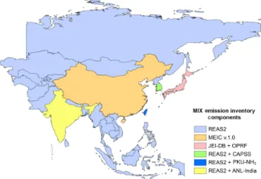
Figure 1.Domain and component of the MIX emission inventory.
into the HTAP v2.2 global emission inventory (Janssens-Maenhout et al., 2015) to support the modeling activities in HTAP, providing a consistent emission input for global and regional modeling activities.
Figure 1 presents the definition of the MIX domain and emission datasets used for each country and region. The do-main of MIX covers 29 countries and regions (the full list of country and region names are listed in Table 1), stretching from Kazakhstan in the west to Russia Far East in the east and from Indonesia in the south to Siberia in the north. Emis-sions are aggregated into five sectors: power, industry, resi-dential, transportation, and agriculture. Ten chemical species are included in the MIX inventory, including both gaseous and aerosol species: SO2, NOx, CO, NMVOC (non-methane volatile organic compounds), NH3 (ammonia), PM10 (par-ticulate matter with diameter less than or equal to 10 µm), PM2.5 (particulate matter with diameter less than or equal to 2.5 µm), BC (black carbon), OC (organic carbon), and CO2. Only emissions from anthropogenic sources are in-cluded in MIX. NMVOC emissions are speciated into model-ready inputs for two chemical mechanisms: CB05 (the Car-bon Bond mechanism; Yarwood et al., 2005) and SAPRC-99 (the State Air Pollution Research Center 1SAPRC-999 version; Carter, 2000) (see Tables S1 and S2 in the Supplement). Monthly emissions are provided by sector at 0.25◦×0.25◦ resolution. Gridded emissions are available from http://www. meicmodel.org/dataset-mix. The key features of the MIX in-ventory are summarized in Table 1.
This paper documents the methodology and emission datasets of the MIX Asian anthropogenic emission inven-tory. The regional and national inventories used to develop MIX gridded datasets and the mosaic methodology are pre-sented in Sect. 2. Section 3 presents Asian emissions in 2010 and spatial and temporal variations in emissions. Changes in Asian emissions between 2006 and 2010 are also discussed. Section 4 highlights the major improvements in the new ventory by comparing MIX with other Asian emission
in-ventories. Uncertainties and limitations of the inventory are discussed in Sect. 5. Concluding remarks are provided in Sect. 6.
2 Compilation of the MIX emission inventory 2.1 Methodology
Five emission inventories are collected and incorporated into the mosaic inventory, as listed in the following: REAS inventory version 2.1 for the whole of Asia (referred to as REAS2 hereafter; Kurokawa et al., 2013), the Multi-resolution Emission Inventory for China (MEIC) developed by Tsinghua University (http://www.meicmodel.org), a high-resolution NH3emission inventory by Peking University (re-ferred to as PKU-NH3 inventory hereafter; Huang et al., 2012), an Indian emission inventory developed by Argonne National Laboratory (referred to as ANL-India hereafter; Lu et al., 2011; Lu and Streets, 2012), and the official Korean emission inventory from the Clean Air Policy Support Sys-tem (CAPSS; Lee et al., 2011).
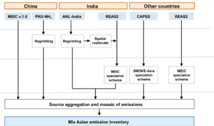
We then selected different emission datasets for various species for each country by the following hierarchy. REAS2 was used as the default where local emission data are ab-sent. Emission inventories compiled by the official agencies or developed with more local information are selected to override REAS2, which include MEIC for mainland China, ANL-India for India, and CAPSS for the Republic of Ko-rea. Detailed information and advantages of these invento-ries are presented in Sect. 2.2. As only a few species (SO2, BC, OC, and power plant NOx)were available from ANL-India, REAS2 was used to supplement the missing species. A mosaic process was then used to combine ANL-India and REAS2 into a single dataset for Indian emissions. It is worth noting that the REAS2 has incorporated local inventories for Japan and Taiwan, which are subsequently adopted in MIX for these two regions. PKU-NH3was further used to replace MEIC emissions for NH3over China, given that PKU-NH3 was developed with a process-based model that represented the spatiotemporal variations in NH3emissions. Table 2 lists the information of each inventory used in MIX.
Figure 2 illustrates the mosaic process for the MIX inventory development. Each dataset was reprocessed to 0.25◦×0.25◦resolution with monthly variations when
nec-essary. We used monthly gridded emissions from each com-ponent inventory where available and assumed no monthly variation in emissions when the component inventory only provided annual emissions. The monthly profiles and spa-tial proxies used in each component emission inventories are summarized in Tables S3 and S4.
Table 1.Summary of the MIX Asian anthropogenic emission inventory.
Item Description
Domain 29 countries and regions in Asia
Countries and regions China, Japan, Democratic People’s Republic of Korea, Republic of Korea, Mongolia, India, Afghanistan, Bangladesh, Bhutan, Maldives, Nepal, Pakistan, Sri Lanka, Brunei, Cambodia, Indonesia, Laos, Malaysia, Myanmar, Philippines, Singapore, Thailand, Vietnam, Kazakhstan, Kyrgyzstan, Tajikistan, Turkmenistan, Uzbekistan, Russia (East Siberia, Far East, Ural, West Siberia)
Species SO2, NOx, CO, NMVOC, NH3, PM10, PM2.5, BC, OC, CO2 VOC speciation by chemical mechanisms: CB05, SAPRC-99
Sectors power, industry, residential, transportation, agriculture Spatial resolution 0.25◦×0.25◦
Seasonality monthly
Year 2008, 2010
Data Access http://www.meicmodel.org/dataset-mix
Table 2.List of regional emission inventories used in this work.
MEIC v1.0 PKU-NH3 CAPSS JEI-DB+OPRF ANL-India REAS2
Year 1990–2010 2006 2008, 2010 2008, 2010 1996–2010 2008, 2010 2000–2010
Region China China Republic of Korea Japan India India Asia
Seasonality Monthly Monthly Annual Monthly Monthly Annual Monthly
Resolution 0.25◦∗ 1 km 0.25◦ 1 km 0.1◦ 0.25◦∗ 0.25◦∗
SO2 X X X X X
NOx X X X X X
CO X X X X
NMVOC X X X X
NH3 X X X X
PM10 X X X X
PM2.5 X X X
BC X X X X
OC X X X X
CO2 X X X X
NMVOC speciation X X
∗Power plant emissions are developed with specific geophysical locations and allocated into 0.25◦×0.25◦grids.
Figure 2.Schematic methodology of the MIX emission inventory development.
from subsectors to the five MIX sectors for each regional in-ventory. For each subsector, the corresponding IPCC sectors are also provided in Table S5. For agriculture sector, only NH3emissions are provided in the MIX inventory given that soil NOx emissions and agriculture PM emissions are not available in the regional inventories used for compiling MIX. Emissions from open biomass burning, fugitive dust, avia-tion, and international shipping were excluded in the MIX inventory because those emissions were only available in a few inventories.
Figure 3.NMVOC speciation scheme used in the MIX inventory development. The mapping table is derived from Carter (2013).
2.2 Components of the MIX emission inventory 2.2.1 REAS2
We used anthropogenic emissions from REAS2 (Kurokawa et al., 2013) to fill the gap where local emission data are not available. REAS2 updated the REAS version 1.1 for both ac-tivity data and emission factors by each country and region using global and regional statistics and recent regional spe-cific studies on emissions factors. Improved from its previ-ous version, power plant emissions in REAS2 were estimated by combining information on generation capacity, fuel type, running years, and CO2 emissions from the Carbon Moni-toring for Action database (CARMA; Wheeler and Ummel, 2008) and the World Electric Power Plants database (WEPP; Platts, 2009). REAS2 extended the domain to include emis-sions of Central Asia and the Asian part of Russia (referred to as Russia Asia). Readers can refer to Kurokawa et al. (2013) for detailed data sources of activity rates and emission fac-tors assignments for each country and source type. REAS2 is available for the period of 2000–2008. In this work, we updated the REAS2 to the year 2010, following the same ap-proach documented in Kurokawa et al. (2013).
REAS2 also incorporated a few regional inventories devel-oped by local agencies with detailed activity data and emis-sion factors, including the JEI-DB inventory (Japan Auto-Oil Program (JATOP) Emission Inventory-Data Base; JPEC, 2012a, b, c) for all anthropogenic sources in Japan excluding shipping, OPRF (Ocean Policy Research Foundation; OPRF, 2012) for shipping emissions in Japan, CAPSS emission in-ventory for Korea (Lee et al., 2011), and official emission data from the Environmental Protection Administration of Taiwan for Taiwan (Kurokawa et al., 2013). All these re-gional datasets were then harmonized to the same spatial and temporal resolution in REAS2. In this work, we processed the CAPSS emission data separately as an individual data
source, which is presented in Sect. 2.2.5, and adopted Japan and Taiwan emissions directly from the REAS2 product.
The REAS2 inventory is provided with monthly gridded emission data for both air pollutants and CO2 by sectors at 0.25×0.25◦ resolution. We aggregated the 11 REAS2 sectors to 5 sectors provided in the MIX inventory. Emis-sions from open biomass burning, aviation, and international shipping were excluded from the REAS2 before incorporat-ing into MIX. Monthly variations are developed for power plants, industry, residential sources, and cold-start emissions from vehicles by various monthly profiles (Kurokawa et al., 2013). In REAS2, power plants with annual CO2emissions larger than 1 Tg were provided as point sources with coor-dinates of locations, while emissions for other sectors were processed as areal sources and gridded at 0.25×0.25◦
reso-lution using maps of rural, urban, and total populations and road networks (see Table S4).
2.2.2 MEIC
We use anthropogenic emission data generated from the MEIC (Multi-resolution Emission Inventory for China) model to override emissions in mainland China. MEIC is a bottom-up emission inventory framework developed and maintained by Tsinghua University, which uses a technology-based methodology to calculate air pollutant and CO2 emissions for more than 700 anthropogenic emitting sources for China from 1990 to the present. With the detailed source classification, the MEIC model can represent emis-sion characteristics from different sectors, fuels, products, combustion/process technologies, and emission control tech-nologies. The MEIC model improved the bottom-up emis-sion inventories developed by the same group (Streets et al., 2006; Zhang et al., 2007a, b, 2009; Lei et al., 2011) and inte-grated them into a uniform framework. The major improve-ments include a unit-based power plant emission database (Wang et al., 2012; Liu et al., 2015), a high-resolution ve-hicle emission modeling approach (Zheng et al., 2014), an explicit NMVOC speciation assignment methodology (Li et al., 2014), and a unified, online framework for emission cal-culation, data processing, and data downloading (available at http://www.meicmodel.org).
County-level emissions were further allocated to high-resolution grids based on a digital road map and weighting factors of vehicle kilometers traveled by vehicle and road type.
MEIC provides lumped speciated NMVOC emissions for different chemical mechanisms, e.g., 99, SAPRC-07, CBIV, CB05, and RADM2. Following the speciation assignment approach developed by Li et al. (2014), emis-sions of individual NMVOC species were calculated for each source category by splitting the total NMVOC emissions with corresponding source profiles. Emissions were then as-signed to various mechanisms using species mapping tables. MEIC delivers monthly emissions at various spatial res-olutions through an open-access, online framework (http:// www.meicmodel.org). Monthly variations and gridded emis-sions were generated by sector using different temporal profiles and spatial proxies. Users can define the metadata (species, domain range, time period, sectors, spatial reso-lution, and chemical mechanisms), calculate gridded sions, and download data from the website. Monthly emis-sions at 0.25◦×0.25◦ generated from MEIC v1.0 (referred to as MEIC hereafter) were used in MIX. Emissions were aggregated to four MIX sectors: power, industry, residential, and transportation. NH3 emissions in MEIC were replaced by PKU-NH3, which will be discussed in the next section.
2.2.3 PKU-NH3for China
We used a high-resolution NH3emission inventory in China compiled by Peking University (PKU-NH3; Huang et al., 2012) to replace China’s NH3 emissions in MEIC. MEIC used annual and regional average NH3 emission factors to calculate emissions from each source category, while PKU-NH3used a process-based model to estimate NH3emissions which parameterized the spatial and temporal variations of emission factors with consideration of ambient temperature, soil property, and other factors. For NH3emissions from fer-tilizer applications, ferfer-tilizer type, soil property, ferfer-tilizer ap-plication method, apap-plication rate, and ambient temperature were used to develop monthly and gridded emission fac-tors. For livestock wastes, emissions were estimated based on a mass-flow methodology by tracing the migration and volatilization of nitrogen from each stage of livestock ma-nure management.
PKU-NH3 estimated NH3 emissions in China (includ-ing mainland China and Hong Kong, Macao, and Taiwan) in 2006 for the following sources: livestock wastes, farm-land ecosystem, biomass burning, excrement from rural pop-ulation, chemical industry, waste disposal, and transporta-tion. Open biomass burning was excluded from the MIX inventory aggregation since the MICS-Asia III project uses GFED dataset for biomass burning. PKU-NH3 is available at 1 km×1 km resolution with monthly variation. We then regridded PKU-NH3monthly emissions to 0.25◦×0.25◦. In the MIX inventory, 2006 emissions from PKU-NH3are used for both 2008 and 2010 since 2006 is the most recent year
for emissions in PKU-NH3when the MIX inventory was de-veloped. As the major drivers of NH3 emissions, synthetic fertilizer consumption and animal population increased by 4 and 9 % from 2006 to 2010, respectively, much smaller than the growth rates of coal consumption and vehicle population for the same period.
2.2.4 ANL emission inventories for India
A high-resolution Indian emission inventory developed by ANL (referred to as ANL-India hereafter; Lu et al., 2011) was used in the MIX inventory. ANL-India used a technology-based methodology to estimate SO2, BC, and OC emissions in India for the period of 1996–2010. Ma-jor anthropogenic sources including both fossil-fuel and bio-fuel combustion are covered in ANL-India. Time-dependent trends in emission factors were developed by taking account of the impact of technology changes on emissions (Habib et al., 2004; Venkataraman et al., 2005). Lu and Streets (2012) further updated power plant emissions in India by calculating emissions at the generating unit level (∼800 units in total) based on information from the reports of the Central Electric-ity AuthorElectric-ity (CEA), including geographical location, capac-ity, fuel type, electricity generation, time the plant was com-missioned/decommissioned, etc. The exact location of each power plant was obtained from the Global Energy Observa-tory (http://globalenergyobservaObserva-tory.org) and crosschecked through Google Earth. The updated unit-based power plant emissions in ANL-India are available for SO2, NOx, BC, and OC.
ANL-India is available for the period of 1990–2010 at 0.1◦×0.1◦ resolution with monthly variations. Emissions
are presented by sectors, i.e., power, industry, residential, transportation, and open biomass burning. Monthly varia-tions in ANL-India were developed by sector using vari-ous surrogates (Lu et al., 2011). As ANL-India only covers some of the required MIX species (SO2, BC, and OC for all sectors, NOx for power plants), monthly emissions by sec-tor (excluding open biomass burning) from ANL-India were first regridded to 0.25◦×0.25◦and then merged with REAS2 before being implemented in MIX to cover all species. The merge process is presented in Sect. 2.3.
ratios to estimate PM2.5, BC, and OC emissions. In the MIX inventory, we used the 2008 and 2009 CAPSS inventories to represent 2008 and 2010 emissions of the Republic of Korea, because 2009 is the most recent year of CAPSS inventory at the time the MIX inventory was developed. In the CAPSS inventory, point sources, area sources, and mobile sources were processed using different spatial allocation approaches (Lee et al., 2011). We used the 0.25◦×0.25◦emission prod-uct from CAPSS as input for the MIX inventory. Only annual total emissions were presented in the CAPSS inventory. In the MIX inventory, we assume no monthly variation in emis-sions in the Republic of Korea.
2.3 Mosaic of Indian emission inventory
ANL-India is available for SO2, BC, and OC for all sectors as well as NOx for power plants. In this work, REAS2 is used to supplement the missing species in ANL-India. To reduce possible inconsistencies from implementation of the two different inventories, we have reprocessed ANL-India and REAS2 emissions over India in the following two steps. First, for power plants, because ANL-India used CEA re-ports to derive information of individual power generation units while REAS2 used the CARMA and WEPP databases to get similar information, direct merging of the two prod-ucts could introduce inconsistency due to a mismatch of unit information in the two databases. In this work, we directly used ANL-India for SO2, NOx, BC, and OC emissions and used REAS2 for CO, NMVOC, PM2.5, PM10, and CO2but redistributed the total magnitudes of REAS2 power plant emissions by using the spatial distribution of power plants in the ANL-India inventory. We generated the spatial proxies of fuel consumption for each fuel type (coal, oil, and gas) at 0.25×0.25◦ by aggregating fuel consumptions of each unit in the ANL-India inventory. We then applied the spa-tial proxy to the REAS2 estimates by fuel type for species that were not included in ANL-India.
Second, we used BC and OC emissions from ANL-India but used PM2.5 and PM10 emissions from REAS2. In cer-tain grids, the sum of BC and OC emissions may exceed PM2.5 emissions because the two inventories may use dif-ferent activity data, emission factors, and spatial proxies. The so-called “PMfine” species in chemical transport models are usually calculated by subtracting BC and OC emissions from total PM2.5emissions, leading to negative emissions of PMfine in those grids. In this case, we adjusted the emissions of PM2.5to the sum of BC and OC emissions for each sector.
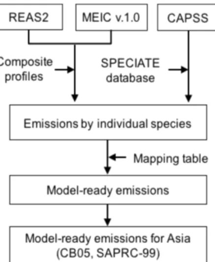
2.4 NMVOC speciation of the MIX inventory
In the MIX inventory, we provide model-ready speciated NMVOC emissions over Asia (except the Republic of Ko-rea) for both CB05 and SAPRC-99 chemical mechanisms, by using the explicit species mapping approach and updated NMVOC profiles developed in Li et al. (2014), as illustrated
in Fig. 3. Following Li et al. (2014), NMVOC emissions for CB05 and SAPRC-99 species are calculated as follows:
EVOC(i, k, m)= n
X
j=1
EVOC(i, k)×X(i, j )
mol(j ) ×C(j, m)
, (1)
wherekis the region,mis species type in CB05 or SAPRC-99 mechanisms, andnis the number of species emitted from sourcei. EVOC is the total NMVOC emissions by source type. In this work, emissions in China and other Asian coun-tries were derived from MEIC and REAS2 respectively.X(i,j) is the mass fraction of speciesjin the total NMVOC emis-sions for sourcei, which is taken from the profiles developed by Li et al. (2014). Those profiles were constructed by group-ing and averaggroup-ing multiple profiles from both local measure-ments and the SPECIATE database (Hsu and Divita, 2009; Simon et al., 2010). Mol(j)is the mole weight of species j andC(j,m)is the conversion factor betweenjandmobtained from the mapping tables in Carter (2013).
For the Republic of Korea, the SMOKE-Asia model devel-oped by Woo et al. (2012) was used to calculate model-ready NMVOC emissions for both CB05 and SAPRC-99 mecha-nisms. NMVOC emissions from the CAPSS were mapped to Source Classification Codes (SCCs) and country–state– county (FIPS) code in SMOKE-Asia model and speciated NMVOC emissions were then calculated by linking emis-sions to speciation profiles with cross references.
2.5 Monthly profiles
We directly used monthly emissions from each regional emission inventory when compiling the MIX inventory. We assume no monthly variation in emissions when monthly profiles are absent from the regional emission inventories. Table S3 presents the monthly profiles used in each compo-nent emission inventory for MIX. In summary, monthly pro-files for power plant emissions usually developed based on monthly statistics of power generation. Monthly profiles of industrial emissions are derived from monthly output of in-dustrial products or inin-dustrial GDP. Residential monthly pro-files are estimated from stove operation time based on ambi-ent temperatures by regions (Streets et al., 2003).
2.6 Spatial proxies
Figure 4.Emission distributions among sectors in Asia in 2010.
3 Results
3.1 Asian anthropogenic emissions in 2010
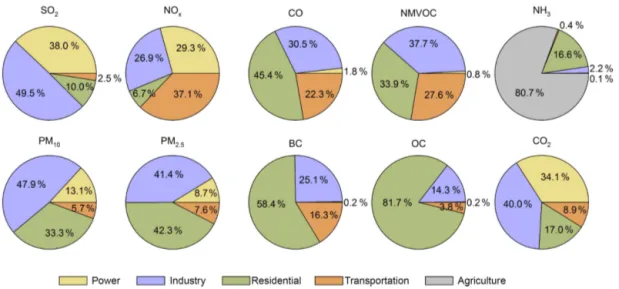
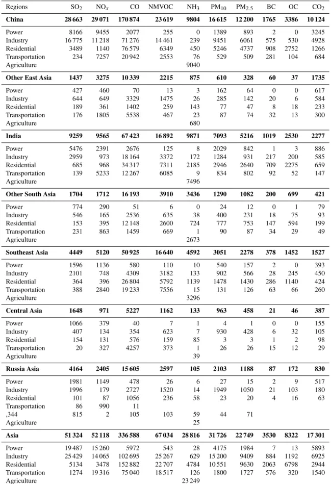
Based on the mosaic approach and candidate inventories de-scribed in Sect. 2, gridded anthropogenic emissions for 10 species were generated over Asia and called the MIX emis-sion inventory. In the MIX inventory, Asian anthropogenic emissions in 2010 are estimated as follows: 51.3 Tg SO2, 52.1 Tg NOx, 336.6 Tg CO, 67.0 Tg NMVOC, 28.8 Tg NH3, 31.7 Tg PM10, 22.7 Tg PM2.5, 3.5 Tg BC, 8.3 Tg OC, and 17.3 Pg CO2. Figure 4 presents the emission distributions among sectors over Asia in 2010. Among the different sec-tors, the industrial sector has the largest contribution to SO2 (50 % of total), NMVOC (38 %), PM10 (48 %), and CO2 (40 %) emissions. Power plants have significant contribu-tions for SO2(38 % of total), NOx (29 %), and CO2(34 %) emissions.
Asian emissions in 2010 for 10 species are listed in Table 3 by country and the shares of 2010 emissions by each subre-gion are presented in Fig. 5. China is the largest contribu-tor for most species except NH3, with more than 50 % con-tribution for SO2, NOx, CO, PM10, PM2.5, and CO2 emis-sions. Following China, India is the largest contributor for NH3 emissions (34 % of total) and the second largest con-tributor for all other species. As shown in Fig. 5, South-east Asia and Other South Asia contribute more than 20 % to NMVOC, NH3, OC, and CO emissions and around 10 % for other species, representing, in particular, a high contribu-tion from biofuel emissions. Contribucontribu-tions from other Asian regions are less than 10 % for all species.
Table 4 presents Asian 2010 emissions by region and by sector. Emissions by country and by sector can be downloaded from the MIX website (http://www.meicmodel. org/dataset-mix.html). China’s anthropogenic emissions in 2010 are estimated as follows: 28.7 Tg SO2, 29.1 Tg NOx,
170.9 Tg CO, 23.6 Tg NMVOC, 9.8 Tg NH3, 16.6 Tg PM10, 12.2 Tg PM2.5, 1.8 Tg BC, 3.4 Tg OC, and 10.1 Pg CO2. Overall, industry is the largest emitter of China’s anthro-pogenic emissions, contributing 49 % of the total CO2 emis-sions and 59, 39, 61, and 50 % of SO2, NOx, NMVOC, and PM2.5emissions respectively. The dominance of the indus-trial sector on China’s anthropogenic emissions reflects the fact that China has developed a huge industrial capacity, which has led to very high levels of energy use and emis-sions. For example, China produced 44 and 70 % of global iron and cement, respectively, in 2010 (World Steel Asso-ciation, 2011; United Nations, 2011). As a result, industrial SO2 emissions in China in 2010 surpassed SO2 emissions from the US and Europe combined. Power plants contributed 32 % of the total CO2emissions and 28, 33, and 7 % of SO2, NOx, and PM2.5 emissions respectively. Emission ratios of SO2/CO2and PM2.5/CO2are lower in power plants than in the industrial sector, reflecting better emission control facili-ties operated in power plants, such as flue-gas desulfurization devices (FGD). The residential sector dominates emissions for pollutants from incomplete combustion, given that large amounts of solid fuels (coal and biomass) were burned in small stoves in China’s homes. The residential sector shared 13 % of China’s total CO2emissions in 2010, but contributed to 45 % of CO, 27 % of NMVOC, 51 % of BC, and 81 % of OC emissions respectively. The transportation sector ac-counted for 25, 12, 11, and 16 % of NOx, CO, NMVOC, and BC emissions respectively. The contribution of the trans-portation sector to China’s CO and NMVOC emissions has substantially decreased during recent years, which will be further discussed in the next section.
indus-Table 3.National anthropogenic emissions in the MIX emission inventory in 2010 (units: Tg for CO2and Gg for other species). Bold values are the total emissions for Asian regions.
Countries SO2 NOx CO NMVOC NH3 PM10 PM2.5 BC OC CO2
Chinaa 28 663 29 071 170 874 23 619 9804 16 615 12 200 1765 3386 10 124
Japan 708 1914 4278 1178 479 114 81 20 8 1107
Korea, DPR 211 238 4488 138 111 264 115 14 17 71
Korea, Republic of 418 1062 838 851 190 124 87 24 8 541
Mongolia 99 62 735 47 97 109 46 2 4 15
Other East Asiab 1437 3275 10 339 2215 875 610 328 60 37 1735
India 9259 9565 67 423 16 892 9871 7093 5216 1019 2530 2277
Afghanistan 3 178 456 141 143 21 20 8 10 2
Bangladesh 133 368 2575 788 1016 342 234 33 121 84
Bhutan 5 13 302 50 41 26 21 4 14 5
Maldives 3 8 151 9 1 0 0 0 0 2
Nepal 30 83 2109 443 254 150 139 27 105 34
Pakistan 1397 946 9279 2112 1859 600 558 114 390 263
Sri Lanka 133 116 1321 367 122 152 111 15 59 31
Other South Asiab 1704 1712 16 194 3910 3435 1290 1082 200 699 421
Brunei 11 12 6 32 8 1 0 0 0 9
Cambodia 26 47 1025 211 134 59 56 11 44 17
Indonesia 1964 2570 23 749 7970 1945 1182 947 178 692 554
Laos 150 41 397 85 87 24 22 4 16 6
Malaysia 365 631 3731 1765 255 216 132 16 35 201
Myanmar 67 91 2705 814 425 165 156 31 125 49
Philippines 503 361 2347 869 413 193 123 15 68 119
Singapore 175 116 162 334 10 7 5 1 1 43
Thailand 614 809 8572 2327 649 495 275 35 149 297
Vietnam 575 442 8231 2234 665 710 562 87 322 232
Southeast Asiab 4449 5120 50 925 16 640 4592 3051 2278 378 1452 1527
Kazakhstan 1050 559 3348 544 41 442 222 13 28 204
Kyrgyzstan 27 35 371 40 12 62 28 2 3 6
Tajikistan 14 25 192 30 15 22 13 1 1 4
Turkmenistan 64 124 417 238 14 64 30 2 3 52
Uzbekistan 493 228 899 310 50 373 165 3 11 121
Central Asiab 1648 971 5227 1162 133 963 458 21 46 387
East Siberia 1649 534 2874 394 23 368 198 14 20 184
Far East 358 489 2681 303 18 223 123 22 25 120
Ural 1480 456 4005 591 22 1047 598 19 75 186
West Siberia 677 926 6045 1310 42 465 269 32 52 340
Russia Asiab 4164 2405 15 605 2597 105 2103 1188 87 172 830
Asia 51 324 52 118 336 588 67 034 28 816 31 726 22 749 3530 8322 17 301
aHong Kong, Macao, and Taiwan are included.bThe Asian region includes the set of countries listed in the section.
trial sector has much lower contributions to emissions com-pared to China, while higher emission contributions from the residential sector are estimated. The differences of the emis-sion patterns between China and India can be attributed to differences in the stage of economic development and the
Table 4.Asian emissions by sector in 2010 for each region (units: Tg for CO2and Gg for other species). Bold values are the total emissions for Asian regions.
Regions SO2 NOx CO NMVOC NH3 PM10 PM2.5 BC OC CO2
China 28 663 29 071 170 874 23 619 9804 16 615 12 200 1765 3386 10 124
Power 8166 9455 2077 255 0 1389 893 2 0 3245
Industry 16 775 11 218 71 276 14 461 239 9451 6061 575 530 4928
Residential 3489 1140 76 579 6349 450 5246 4737 908 2752 1266
Transportation 234 7257 20 942 2553 76 529 509 281 104 684
Agriculture 9040
Other East Asia 1437 3275 10 339 2215 875 610 328 60 37 1735
Power 427 460 70 13 3 162 64 0 0 617
Industry 644 649 3329 1475 26 285 142 20 6 584
Residential 189 361 1402 259 143 77 47 8 18 233
Transportation 176 1805 5538 467 23 87 74 32 13 300
Agriculture 680
India 9259 9565 67 423 16 892 9871 7093 5216 1019 2530 2277
Power 5476 2391 2676 125 8 2029 842 1 3 886
Industry 2959 973 18 164 3372 172 1284 931 217 200 585
Residential 685 968 34 317 7311 2185 2946 2640 709 2275 659
Transportation 139 5233 12 267 6085 9 834 802 92 52 147
Agriculture 7496
Other South Asia 1704 1712 16 193 3910 3436 1290 1082 200 699 421
Power 774 290 51 6 0 24 12 0 1 79
Industry 546 165 2536 635 38 400 231 18 75 93
Residential 153 395 12 148 2600 724 777 753 147 594 199
Transportation 231 863 1459 669 1 90 87 34 29 49
Agriculture 2673
Southeast Asia 4449 5120 50 925 16 640 4592 3051 2278 378 1452 1527
Power 1596 1136 580 110 10 540 157 2 0 393
Industry 2101 748 4309 3182 133 902 566 28 245 450
Residential 364 396 26 804 5792 1139 1478 1430 286 1140 424
Transportation 388 2840 19 233 7556 15 131 126 63 66 260
Agriculture 3296
Central Asia 1648 971 5227 1162 133 963 458 21 46 387
Power 1066 379 40 7 1 4 1 0 0 155
Industry 407 134 354 623 7 930 428 6 32 105
Residential 154 131 576 159 85 3 3 1 2 98
Transportation 20 327 4257 373 1 26 26 15 12 29
Agriculture 39
Russia Asia 4164 2405 15 605 2597 105 2103 1188 87 172 830
Power 1981 1149 478 26 6 27 15 2 9 517
Industry 1996 179 2727 1520 14 1949 1050 21 103 180
Residential 101 87 1056 236 58 23 20 4 16 63
Transportation 86 990 11
,344 815 2 105 103 59 44 71
Agriculture 25
Asia 51 324 52 118 336 588 67 034 28 816 31 726 22 749 3530 8322 17 301
Power 19 487 15 260 5972 543 28 4175 1984 7 13 5893
Industry 25 429 14 065 102 695 25 267 629 15 200 9409 884 1192 6925 Residential 5134 3478 152 882 22 707 4784 10 551 9630 2063 6798 2944 Transportation 1274 19 316 75 040 18 517 126 1800 1727 576 320 1540
Figure 5.Emissions distributions by Asian regions in 2010.
of coal-fired generation units, SO2 emissions from Indian power plants are estimated to be 5.5 Tg in 2010, contribut-ing 59 % of the total Indian SO2emissions. The SO2/CO2 emission ratio in Indian power plants is significantly higher than that of China, representing the low penetration rates of FGD in Indian power plants (Lu et al., 2011). The transporta-tion sector contributes 55 % of NOx and 36 % of NMVOC emissions in India. These large shares are caused by the high emission factors used in REAS2, in which relatively poor emission control measures are in place (Kurokawa et al., 2013).
Figure 6 compared per capita emissions by sector and by species in 2010 for each country. Emissions are ranked by GDP per capita of each country. The correlations between emission intensity (per capita emissions) and economic de-velopment (GDP per capita) at country level are not always significant because emission intensities are affected by not only economic level but also by other factors such as in-dustrial structure and dominant fuel type. Nevertheless, the changes in emission intensities in general follow the pat-tern of Kuznets curve for most species except NH3, BC, and OC. Emission intensities tend to increase following the GDP growth first and then tend to decrease for high-income coun-tries. For BC and OC, per capita emissions are higher in de-veloping countries than in developed countries because low-income countries with low low-incomes tend to use biofuels in which emitted more BC and OC than other fuel types.
Ratios of different species were widely used to inform emission characteristics. For example, SO2/CO2 ratio was used as an indicator of coal combustion and emission control levels (Li et al., 2007), and ratios of CO/CO2 were used to inform combustion efficiency (Wang et al., 2010). Fig-ure 7 compares regional emission ratios of SO2/CO2 and CO/CO2estimated by the MIX inventory. Emission ratios of SO2/CO2are lowest in Other East Asia among different regions, which could be attributed to small share of coal use
and high penetration of emission control facilities, while high emissions ratios of SO2/CO2were found in Russia Asia and Central Asia due to high fraction of coal use and less emis-sion controls. Other East Asia also has the lowest emisemis-sion ratios of CO/CO2among different regions, owing to a high contribution from industrial and transportation emissions. In contrast, high emissions from small residential combustions led to low combustion efficiencies and high emission ratio over India and Southeast Asia.
3.2 Changes of Asian emissions from 2006 to 2010 In this work, we also developed Asian emissions for 2006 and 2008 following the same approach of MIX, to illustrate the changes in Asian emissions from 2006 to 2010. Table 5 presents Asian emissions in 2006 and emission ratios of 2010 to 2016 by country. For the whole of Asia, emission growth rates from 2006 to 2010 are estimated as follows: −8.1 % for SO2, +19.2 % for NOx,+3.9 % for CO, +15.5 % for NMVOC,+1.7 % for NH3, −3.4 % for PM10, −1.6 % for PM2.5, +5.5 % for BC, +1.8 % for OC, and +19.9 % for CO2. Growth in CO2 emissions represent the continuously increasing energy use across Asia during 2006–2010, while different trends among species represents differences in the emission control level among sectors and regions. Compared to the increasing emission trends of all species during 2001– 2006 (Zhang et al., 2009), the relatively flat or even decreas-ing emission trends in many species indicate the effective-ness of emission control measures in recent years (Gu et al., 2013; Lin et al., 2010; Wang et al., 2013).
Figure 6.Per capita emissions by sector for 2010 in MIX, ranked by GDP per capita for each country.
Li
et
al.:
MIX:
a
mosaic
Asian
anthr
opogenic
emission
in
v
entory
947
2
Regions SO2 NOx CO NMVOC NH3 PM10 PM2.5 BC OC CO2
China 34 597 (0.83) 23 719 (1.23) 179 626 (0.95) 20 715 (1.14) 11 203 (0.88) 19 342 (0.86) 13 752 (0.89) 1771 (1.00) 3486 (0.97) 7827 (1.29)
Japan 838 (0.85) 2352 (0.81) 5888 (0.73) 1538 (0.77) 507 (0.94) 149 (0.76) 109 (0.74) 32 (0.63) 12 (0.68) 1241 (0.89) Korea, DPR 233 (0.91) 293 (0.81) 5430 (0.83) 175 (0.79) 108 (1.02) 319 (0.83) 139 (0.83) 16 (0.86) 18 (0.94) 84 (0.85) Korea, Republic of 446 (0.94) 1270 (0.84) 827 (1.01) 794 (1.07) 184 (1.03) 65 (1.91) 42 (2.04) 15 (1.55) 12 (0.69) 510 (1.06) Mongolia 71 (1.39) 45 (1.37) 523 (1.4) 37 (1.29) 103 (0.93) 75 (1.46) 31 (1.49) 1 (1.58) 2 (1.72) 11 (1.38)
Other East Asia 1588 (0.90) 3961 (0.83) 12 668 (0.82) 2544 (0.87) 903 (0.97) 607 (1.01) 321 (1.02) 65 (0.92) 44 (0.84) 1846 (0.94)
India 7476 (1.24) 7484 (1.28) 55 910 (1.21) 14 685 (1.15) 9015 (1.09) 5874 (1.21) 4327 (1.21) 887 (1.15) 2415 (1.05) 1892 (1.20)
Afghanistan 2 (1.33) 111 (1.60) 279 (1.64) 96 (1.46) 131 (1.10) 14 (1.49) 13 (1.48) 5 (1.48) 7 (1.37) 2 (1.25) Bangladesh 102 (1.30) 283 (1.30) 2332 (1.10) 711 (1.11) 889 (1.14) 283 (1.21) 203 (1.15) 30 (1.09) 113 (1.07) 67 (1.25) Bhutan 4 (1.32) 11 (1.21) 256 (1.18) 43 (1.15) 42 (0.99) 21 (1.23) 18 (1.18) 3 (1.14) 12 (1.13) 4 (1.17) Maldives 3 (0.97) 8 (0.98) 144 (1.05) 7 (1.21) 0 (1.07) 0 (1.28) 0 (1.27) 0 (1.45) 0 (1.40) 2 (1.00) Nepal 28 (1.08) 72 (1.16) 1985 (1.06) 405 (1.09) 242 (1.05) 138 (1.08) 128 (1.08) 25 (1.08) 98 (1.08) 32 (1.07) Pakistan 1128 (1.24) 816 (1.16) 8298 (1.12) 1871 (1.13) 1543 (1.20) 542 (1.11) 503 (1.11) 103 (1.11) 358 (1.09) 231 (1.14) Sri Lanka 108 (1.23) 120 (0.96) 1274 (1.04) 347 (1.06) 112 (1.09) 123 (1.23) 98 (1.13) 15 (1.00) 58 (1.02) 29 (1.08)
Other South Asia 1376 (1.24) 1421 (1.20) 14 568 (1.11) 3481 (1.12) 2959 (1.16) 1121 (1.15) 964 (1.12) 181 (1.10) 647 (1.08) 365 (1.15)
Brunei 9 (1.22) 10 (1.15) 6 (0.91) 32 (0.98) 7 (1.13) 1 (0.56) 1 (0.58) 0 (0.67) 0 (0.53) 8 (1.18) Cambodia 26 (0.99) 46 (1.00) 976 (1.05) 198 (1.07) 121 (1.11) 55 (1.06) 53 (1.06) 11 (1.04) 42 (1.04) 16 (1.04) Indonesia 1676 (1.17) 1999 (1.29) 19 379 (1.23) 6134 (1.30) 1634 (1.19) 1237 (0.96) 944 (1.00) 164 (1.08) 663 (1.04) 520 (1.07) Laos 133 (1.13) 35 (1.17) 388 (1.02) 80 (1.06) 78 (1.12) 24 (1.01) 22 (1.01) 4 (1.02) 16 (1.00) 6 (1.03) Malaysia 290 (1.26) 505 (1.25) 3117 (1.20) 1504 (1.17) 222 (1.15) 191 (1.13) 126 (1.05) 14 (1.13) 33 (1.05) 175 (1.15) Myanmar 71 (0.94) 76 (1.21) 2594 (1.04) 654 (1.25) 392 (1.08) 155 (1.06) 149 (1.04) 30 (1.04) 121 (1.03) 47 (1.05) Philippines 474 (1.06) 288 (1.26) 2269 (1.03) 812 (1.07) 404 (1.02) 160 (1.21) 114 (1.08) 15 (0.97) 70 (0.98) 94 (1.27) Singapore 191 (0.92) 112 (1.03) 138 (1.18) 290 (1.15) 12 (0.85) 7 (0.96) 6 (0.97) 1 (1.08) 1 (1.12) 39 (1.08) Thailand 796 (0.77) 740 (1.09) 7555 (1.13) 2031 (1.15) 533 (1.22) 508 (0.97) 285 (0.96) 33 (1.06) 134 (1.11) 271 (1.09) Vietnam 463 (1.24) 337 (1.31) 7419 (1.11) 1584 (1.41) 624 (1.07) 594 (1.20) 485 (1.16) 79 (1.09) 302 (1.06) 184 (1.26)
Southeast Asia 4129 (1.08) 4149 (1.23) 43 841 (1.16) 13 319 (1.25) 4027 (1.14) 2933 (1.04) 2184 (1.04) 352 (1.07) 1383 (1.05) 1360 (1.12)
Kazakhstan 1775 (0.59) 499 (1.12) 2107 (1.59) 423 (1.28) 39 (1.06) 381 (1.16) 192 (1.16) 10 (1.26) 24 (1.17) 191 (1.07) Kyrgyzstan 30 (0.90) 27 (1.32) 224 (1.66) 30 (1.34) 12 (1.00) 60 (1.03) 27 (1.05) 1 (1.44) 2 (1.21) 5 (1.19) Tajikistan 11 (1.24) 16 (1.62) 122 (1.57) 25 (1.17) 15 (1.06) 28 (0.80) 15 (0.86) 1 (1.78) 1 (1.34) 3 (1.03) Turkmenistan 45 (1.42) 97 (1.28) 298 (1.40) 174 (1.37) 13 (1.10) 54 (1.18) 25 (1.20) 2 (1.37) 2 (1.28) 42 (1.22) Uzbekistan 590 (0.84) 241 (0.94) 808 (1.11) 287 (1.08) 53 (0.94) 325 (1.15) 143 (1.15) 3 (1.03) 9 (1.13) 129 (0.94)
Central Asia 2451 (0.67) 879 (1.10) 3558 (1.47) 940 (1.24) 131 (1.01) 847 (1.14) 402 (1.14) 17 (1.27) 39 (1.17) 370 (1.04)
East Siberia 1711 (0.96) 482 (1.11) 2437 (1.18) 351 (1.12) 24 (0.97) 380 (0.97) 199 (0.99) 11 (1.28) 19 (1.06) 178 (1.03) Far East 349 (1.02) 410 (1.19) 2284 (1.17) 268 (1.13) 20 (0.91) 228 (0.98) 120 (1.03) 17 (1.34) 22 (1.13) 109 (1.10) Ural 1510 (0.98) 412 (1.11) 3757 (1.07) 551 (1.07) 22 (0.99) 1042 (1.01) 580 (1.03) 17 (1.09) 69 (1.09) 174 (1.07) West Siberia 647 (1.05) 815 (1.14) 5399 (1.12) 1206 (1.09) 43 (0.99) 484 (0.96) 275 (0.98) 27 (1.19) 50 (1.03) 308 (1.10)
Russia Asia 4217 (0.99) 2119 (1.13) 13 878 (1.12) 2376 (1.09) 108 (0.97) 2132 (0.99) 1173 (1.01) 72 (1.21) 160 (1.07) 770 (1.08)
Asia 55 832 (0.92) 43 732 (1.19) 324 049 (1.04) 58 059 (1.15) 28 348 (1.02) 32 857 (0.97) 23 124 (0.98) 3345 (1.06) 8174 (1.02) 14 430 (1.20)
.atmos-chem-ph
ys.net/17/935/2017/
Atmos.
Chem.
Ph
ys.,
17,
935–
963
,
Figure 8.Emission changes from 2006 to 2010 by Asian regions for SO2(a)and CO(b). Left panel: emissions in 2006 and 2010 by region. Y axis represents emissions by region.Xaxis represents accumulative emission contribution of regions. The dotted and solid lines represent emissions in 2006 and 2010 respectively. Right panel: the shares of emissions by sectors over China and India in 2006 and 2010.
total primary energy consumption of Asia has increased by 20.6 % during the period of 2005 and 2010 (IEA, 2013). During the same period, SO2emissions decreased in China (−17.2 %), Other East Asia (−9.5 %), and Central Asia (−32.8 %) due to effective emission control, while they in-creased in India (+23.9 %), Other South Asia (+23.9 %), and Southeast Asia (+7.8 %) due to growth in coal use and ab-sence of desulfurization devices. The decrease in SO2 emis-sions changes in Asian is dominated by changes in China and India. Figure 8a demonstrates the changes in SO2 emis-sions among Asian regions from 2006 to 2010. Wide in-stallation of FGD in China’s coal-fired power plants is the main driving factor of SO2emission changes over Asia. SO2
in-Table 6.Comparison of emission trends of NOx, SO2, and CO over Asia with satellite observations.
Species Regions Study Method Period AGR (% yr−1)a
NOx China Berezin et al. (2013) Inverse modeling 2001–2008 11.5
China Gu et al. (2013) Inverse modeling 2005–2010 4.0
China Miyazaki et al. (2016) Inverse modeling 2005–2010 3.7
East China Mijling et al. (2013) Inverse modeling 2007–2011 9.0
East China Krotkov et al. (2016) Satellite 2005–2010 5.4
Central East China Itahashi et al. (2014) Satellite 2000–2010 11.0
China This work Inventory 2006–2010 5.2
India Krotkov et al. (2016) Satellite 2005–2010 4.6
India Miyazaki et al. (2016) Inverse modeling 2005–2010 3.2
India This work Inventory 2006–2010 6.3
SO2 East China Krotkov et al. (2016) Satellite 2005–2010 −6.9
China This work Inventory 2006–2010 −4.6
India Krotkov et al. (2016) Satellite 2005–2010 16.5
India This work Inventory 2006–2010 5.5
CO China Yumimoto et al. (2014) Inverse modeling 2005–2010 −3.1
China Yin et al. (2015) Inverse modeling 2002–2011 −1.1
East China Worden et al. (2013) Satellite 2000–2012 −1.6,−1.0b
China This work Inventory 2006-2010 −1.2
aAGR is annual growth rate.bResults are developed using MOPITT and AIRS.
dustrial activities and vehicle population. For NOx, remark-able emission increases are observed for China (+22.6 %), India (+27.8 %), Other South Asia (+20.5 %), and South-east Asia (+23.4 %) during 2006–2010. For NMVOC, emis-sions increased by 14.0, 15.0, 12.3, 24.9, 23.6, and 9.3 % for China, India, Other South Asia, Southeast Asia, Cen-tral Asia, and Russia Asia respectively. Emission changes of other species are relatively small (i.e., within 6 %) during 2006–2010. For CO, PM10, and PM2.5, emission reductions in China were partly offset by increases of emissions in the South and Southeast Asian regions. CO emissions in China decreased by 5 % during 2006–2010 (see Fig. 8b), mainly due to improved combustion efficiency, recycling of indus-trial coal gases, and strengthened vehicle emission standards. The implementation of new vehicle emission standards and retirement of old vehicles has reduced China’s transportation CO and NMVOC emissions by 20 and 30 %, respectively, during 2006–2010. While in India, Other South Asia, and Southeast Asia, CO emissions increased by 21, 11, and 16 %, respectively, between 2006 and 2010.
Satellite observations have shown promising capabilities in detect trends in surface emissions (Streets et al., 2013). The increases in NOx emissions over China and India were confirmed by satellite-based inversions and the growth rates in satellite-based NOx emission trends during 2006–2010 are generally comparable to our estimates in emission in-ventories (Table 6). For SO2emissions, the downward trend over China and upward trend over India were also observed by satellite remote sensing, while higher growth rates were detected by OMI than the bottom-up emission inventory
(Krotkov et al., 2016). The downward trend of CO emissions over China in recent years has been confirmed by both in situ and satellite observations (Wang et al., 2010; Worden et al., 2013; Yumimoto et al., 2014; Yin et al., 2015). The de-creasing rate of CO emissions over China is estimated to be −1.2 % yr−1from 2006 to 2010 in the MIX inventory, con-sistent with the rates observed by multiple satellites in range of−1.0 to−3.1 % yr−1during 2000–2012 (Table 6).
3.3 Speciated NMVOC emissions
Figure 9.Speciated NMVOC emissions for the year 2010 by chemical group and by Asian regions. Alkanes: ethane, propane, butanes, pentanes, hexanes, higher alkanes and their isomers. Alkenes: ethane, propene, isoprene, terpenes, higher alkenes and their isomers. Alkynes: ethyne and other alkynes. Aromatics: benzene, toluene, xylene, trimethylbenzene, other aromatics and their isomers. OVOCs: aldehydes (formaldehyde, acetaldehyde, and higher aldehydes), ketones (acetone and higher ketones), alcohols (methanol, ethanol, and higher alcohols), ethers, and acids. “Others”: halogenated hydrocarbons, unidentified species, etc.
refinery (15.0 %), and aromatics emissions are mainly con-tributed by architectural paint use (21.0 % of total industrial emissions), other industrial paint use (16.6 %), and gas pro-duction and distribution (10.6 %). The residential sector has a high contribution of OVOCs, alkynes, and alkenes, among which mainly contributed by biofuel combustions. The sec-toral contribution to different chemical groups also varies with region. For example, the residential sector dominates emissions for all species in the Other South Asia region, as a consequence of the low economic development in that re-gion.
Among different regions, China, India, and Southeast Asia are the largest contributors to NMVOC emissions in Asia,
Figure 10.Monthly variations of Asian SO2, CO, PM2.5, and CO2emissions by sector for the year 2010.
3.4 Seasonality
Monthly emissions by sector and by Asian region are pro-vided in Tables S6–S14. Monthly profiles in emissions are highly sector dependent given that monthly activity rates vary among different sectors. Figure 10 illustrates the monthly variations of Asian SO2, CO, PM2.5, and CO2 emis-sions by sector for the year 2010. Different species generally show similar monthly emission patterns within the same sec-tor, indicating that monthly emission profiles of each sector are dominated by monthly variations in activity rates. For ex-ample, industrial emissions are higher in the second half of the year induced by larger industrial productions to meet the annual total production target. The most significant monthly variation with a winter peak was found in the residential sec-tor, reflecting the higher energy demand for residential heat-ing in winter. Residential SO2 emissions in winter are even higher than other species, because SO2emissions from China dominate residential emissions in Asia (70 % of total), of which coal consumption in winter is higher than other re-gions for heating. Monthly profiles of CO emissions are dif-ferent from other species for the transportation sector. This is because the CO emission factor in winter is higher than in other seasons due to additional emissions from the cold-start process (Kurokawa et al., 2013; Zheng et al., 2014).
Figure 11 presents monthly variations of SO2, CO, PM2.5, and CO2 emissions by Asian region. Compared to other
species, CO emissions are much higher in winter in high-latitude regions due to residential heating and additional ve-hicle emissions from cold starts. Winter PM2.5emissions in China are higher than other regions, representing large emis-sions from solid fuel use in residential homes.
3.5 Gridded emissions
In the MIX inventory, gridded emissions for 10 gaseous and aerosol species were developed at 0.25×0.25◦ resolution. Emission maps of all species in 2010 are shown in Fig. 12. Compared to the previous gridded Asian emission invento-ries, we believe the spatial patterns are improved because several local high-resolution emission datasets are incorpo-rated, such as CPED for China and JEI-DB and OPRF for Japan. However, for sectors in which emissions are domi-nated by spatially scattered sources (e.g., residential com-bustion, solvent use), the spatial distributions in emissions are still uncertain.
in-Figure 11.Monthly variations of SO2, CO, PM2.5, and CO2emissions by Asian region for the year 2010.
Table 7.Intercomparisons of total anthropogenic emissionsaamong MIX, REAS2, and EDGAR v4.2 for 2008.
Unit: Tg yr−1 SO2 NOx CO NMVOC NH3 PM10 PM2.5 BC OC CO2
Asiab
MIX 49.00 46.38 317.11 60.26 27.66 30.16 21.71 3.40 8.04 15 145
REAS2 52.82 46.17 344.20 65.94 32.74 34.21 23.51 2.95 7.55 15 271
EDGAR v4.2 63.26 36.73 212.16 53.43 20.08 31.08 15 282
China
MIX 31.41 26.55 175.64 22.10 9.80 17.63 12.74 1.76 3.38 8955
REAS2 33.58 25.55 202.71 27.78 15.00 21.69 14.57 1.60 3.09 9085
EDGAR v4.2 41.35 20.66 106.10 22.60 11.11 14.76 8647
India
MIX 8.42 8.86 61.80 15.95 9.42 6.65 4.88 0.98 2.48 2103
REAS2 10.08 9.68 61.80 15.95 9.42 6.65 4.88 0.71 2.29 2103
EDGAR v4.2 8.42 6.37 45.58 10.58 4.14 10.80 2307
aIncluding power, industry, residential, transportation, and agriculture.b“Asia” refers to all Asian regions excluding the Russia Asia in MIX.
ventory has been regridded to 0.1×0.1◦ resolution using the area-weighting approach and then incorporated to the HTAP v2 gridded emission inventory (Janssens-Maenhout et al., 2015). The HTAP v2 emission inventory can be down-loaded from the EDGAR website (http://edgar.jrc.ec.europa. eu/htap_v2/index.php?SECURE=_123).
4 Comparison with other inventories
4.1 MIX, REAS2, and EDGAR v4.2 over Asia
Figure 12.
with REAS2 and EDGAR v4.2 (EC-JRC/PBL, 2011), two widely used inventories, to highlight the new findings from the mosaic inventory and identify the potential sources of uncertainties. We choose the year of 2008 to conduct the comparison because emissions after 2008 are not available in either REAS2 or EDGAR v4.2. Russian Asia was ex-cluded from comparison. Asian anthropogenic emissions of MIX, REAS2, and EDGAR v4.2 in 2008 are tabulated in Ta-ble 7. Over Asia, MIX and REAS differ within 10 % for most species, except for NH3(18 % higher in REAS), PM10(13 % higher), and BC (13 % lower). It is not surprising that the total Asian emission budgets in MIX and REAS2 are
simi-lar given that MIX used emissions estimates in REAS2 for Asian regions except China and India. However, REAS2 has incorporated several recent emission inventories for China (Kurokawa et al., 2013). The differences between REAS and MIX over China and India will be discussed in the following sections.
differ-Figure 12.Grid maps for gaseous(a)and aerosol(b)species in the MIX Asian emission inventory, 2010.
ences by region and by sector. Regionally, the differences can be largely attributed to disagreements in emission esti-mates for China and India, as presented in Table 7. Discrep-ancies are relatively large at the sector level compared to to-tal emissions. EDGAR’s estimates for SO2 emissions from power plants are 60 % higher than estimates in MIX. For China, 70 % of power generation capacities were equipped with FGD and the average SO2removal efficiency was 78 % (Liu et al., 2015). The high estimates in EDGAR v4.2 are most likely due to underestimation of FGD penetration or SO2removal efficiencies of FGD (Kurokawa et al., 2013). Remarkable differences for the residential and transportation sectors are found for NOx, CO, and NMVOC estimates in the two inventories. For instance, EDGAR v4.2 estimates lower NOx emissions of transportation sector by 27 and by 48 % for the residential sector compared to MIX. Similarly, resi-dential CO emissions in EDGAR v4.2 are 33 % lower than in MIX, leading to 33 % lower estimates of CO emissions in EDGAR v4.2 compared to MIX. Underestimates of CO emissions in EDGAR v4.2 inventory have been confirmed by top-down constraints (Pétron et al., 2004; Fortems-Cheiney et al., 2011). As the statistical differences of energy use are usually within 30 % at sector level (Guan et al., 2012), the discrepancy by sector could only be attributed to differences in the raw emission factors and abatement measures.
Al-though a point-by-point comparison of emission factors be-tween EDGAR v4.2 and MIX is not feasible, we can still speculate that EDGAR v4.2 may overestimate the combtion efficiency and emission control measures in Asia by us-ing an emission factor database from developed countries. NH3emissions in EDGAR v4.2 are 26 % lower than in MIX, with a large difference in residential emissions. The differ-ences are mainly from high emission estimates of wastew-ater treatment sources in REAS2, which were incorporated into MIX for Asian regions except China. MIX estimated 3.4 Tg NH3 emissions from wastewater treatment in Asia in 2008, which are more than 2 orders of magnitude higher than EDGAR v4.2 estimates. Differences in PM10emissions at the sector level are also large; similar estimates of PM10 emissions in the two datasets are rather a coincidence than real agreements.
Figure 13.Intercomparisons of emission estimates between MIX, REAS2, and EDGAR v4.2 by Asian regions and sectors.(a)Absolute differences of emission estimates.(b)Ratio of emission estimates. Grey shaded grids indicate that the comparison is not available due to absence of emission estimates in EDGAR v4.2. Abbreviations of Asian countries and regions are the same as in Fig. 7. Abbreviations of sectors are as follows: POW is power plants; INDU is industry; RES is residential; TRA is transportation; AGR is agriculture; SUM is total. Russia Asia is not included in the comparison.
+13.6 % compared to MIX) but lower emissions for in-dustry (−293 Tg, −6.8 %) emissions. EDGAR v4.2 esti-mates lower CO2 emissions for China (−308 Tg, −3.4 %) and higher emissions for other regions: +102 Tg (+5.6 %) for Other East Asia,+83.9 Tg (+5.6 %) for Southeast Asia, +204 Tg (+9.7 %) for India,+29.5 Tg (+7.5 %) for Other South Asia, and+25.3 Tg (+6.4 %) for Central Asia. At sec-tor level, EDGAR v4.2 estimates are 29 % (+833 Tg) higher for power, 22 % (−944 Tg) lower for industry, and 31 % (−192 Tg) lower for transportation over China compared to MIX. For Other East Asia, differences between EDGAR v4.2 and MIX are mainly contributed by power sector, with 20 % higher emissions (+130 Tg) in EDGAR v4.2. Residen-tial sector is the main contributor to the differences between EDGAR v4.2 and MIX over India, with 28 % (+177 Tg) higher emissions estimated in EDGAR v4.2. The relatively large discrepancy at sector level can be attributed to differ-ences in energy statistics and emission factors (Guan et al., 2012; Liu et al., 2015) as well as differences in sector defi-nitions. In particularly, EDGAR v4.2 used fuel consumption data from IEA statistics while MIX and REAS2 used provin-cial level data from Chinese Energy Statistics, which can dif-fer by 20 % at sector level (Hong et al., 2016). Emissions from heating plants are aggregated to the industrial sector in the MIX inventory, while in EDGAR v4.2 heating plants
are aggregated to the energy sector and then compared to the power sector in the MIX inventory. In the future, har-monizing the sector (subsector) definition among global and regional inventories would help to reduce the discrepancy of emission estimates at sector level.
4.2 China
4.2.1 Power plants
Figure 14.Comparison of 2008 power plants emission estimates between MEIC v1.0, REAS2, and EDGAR v4.2 for Shanxi province, China.(a)Spatial distribution of CO2emissions and(b)emission ratios of SO2to CO2. CO2emissions are grouped by colors.
from large plants by wrongly allocating fuel consumptions of small plants to large ones. REAS2 included 380 power plants for China, compared to 2411 plants in MIX, while power plants in REAS2 are large ones which contributed 72 % of CO2emissions in China.
Figure 14a compares CO2 emissions from power plants between MEIC and REAS2 in Shanxi province where a large amount of coal is extracted and combusted in power plants. EDGAR emissions are also presented in Fig. 14a as a refer-ence. For Shanxi province, MIX, REAS2, and EDGAR in-cluded 134, 22, and 24 coal-fired power plants, respectively, demonstrating the omission of many small power plants in REAS2 and EDGAR. In REAS2, only plants with annual CO2 emissions higher than 1 Tg were processed as point sources (Kurokawa et al., 2013). In the three datasets, a total of 6, 13, and 12 power plants in Shanxi province have annual CO2emissions higher than 5 Tg, respectively, indicating sig-nificant emission overestimates for large plants in REAS2 and EDGAR. Moreover, the locations of power plants are not accurate in EDGAR given that CARMA used city cen-ters as the approximate coordinates of power plants (Wheeler and Ummel, 2008). In contrast, coordinates in CPED are
obtained from official sources and crosschecked by Google Earth (Liu et al., 2015); the positions of large power plants in REAS2 are also checked manually (Kurokawa et al., 2013).
Figure 15.Comparisons of spatial distribution of NH3agricultural emissions between MEIC v1.0 and PKU-NH3. Provinces that included in tropical zones are Fujian, Guangdong, Hainan, Guangxi, Guizhou, Hubei, Hunan, Yunnan, Sichuan, Jiangxi, Anhui, Zhejiang, and Jiangsu. Other provinces are treated as temperate ones.
Table 8.NH3agriculture emission estimates for China.
Unit: Tg-NH3yr−1 PKU-NH3 MEIC v1.0 REAS2 EDGAR v4.2 MASAGE_NH3
Year 2006 2008 2008 2008 2005–2008∗
Fertilizer application 3.20 4.40 9.40 8.26 3.64
Live stock 5.30 5.30 2.80 2.31 5.83
∗Averaged estimates during 2005–2008.
4.2.2 Agriculture
The agriculture sector is a dominant source of NH3 emis-sions, mainly contributed by fertilizer applications and ma-nure managements. MIX incorporated the PKU-NH3 inven-tory for China, which estimated agricultural NH3emissions using a process-based model to represent the dynamic im-pact of fertilizer use patterns, meteorological factors, and soil properties (Huang et al., 2012). The new inventory improved on previous studies which used uniform emission factors across time and region. Table 8 compares agricultural NH3 emissions in China estimated in different emission invento-ries. Compared to other work, PKU-NH3yields lower esti-mates for fertilizer application but higher estiesti-mates for ma-nure management. The differences are mainly because PKU-NH3used local correction factors for fertilizer volatilization and manure loss rate (Huang et al., 2012). Top-down in-version of NH3 emissions by adjoint model and deposition fluxes agrees well with Huang et al. (2012), confirming the validity of the process-based model (Paulot et al., 2014).
Besides the magnitude of emissions, a process-based model may also better represent the spatial and temporal variations in emissions. As an example, Fig. 15 compares NH3agricultural emissions for MEIC and the PKU-NH3 in-ventory for different climate zones. MEIC agrees well with PKU-NH3in temperate zones but is significantly higher than PKH-NH3 in tropical zones. The differences in spatial
dis-tributions can be explained by the discrepancies in derived emission factors in the two inventories given that they used the same activity data from the National Bureau of Statis-tics of China (NBSC). MEIC used a higher loss rate of NH3 (20 % for urea) for tropical zones and a lower one (15 %) for temperate zones following Klimont (2001). With full consid-eration of fertilization method and soil acidity by grids and by month, PKU-NH3estimated 9 % average NH3 loss rate for urea for tropical zones and 14 % for temperate zone.
4.2.3 Other sectors
This section further discusses the differences between MIX and REAS2 over China. EDGAR is not compared here be-cause references to the detailed underlying data used in EDGAR are not available. Figure S1 in the Supplement com-pares MIX and REAS2 estimates for China for 2008 by species and by sector. The two inventories generally agree well given that both MEIC and REAS2 incorporate the most recent advances in emission inventory studies in China. The major differences between the two inventories are discussed below with explanation for possible reasons.
new standards to restrict industrial emissions, leading to a downward trend in emission factors after 2005 (Zhao et al., 2013). Emission standards implemented during 2005– 2010 are summarized in Table S15. For the industrial sector, REAS2 adopted CO and PM emission factors from Streets et al. (2006) and Lei et al. (2011), respectively, which represent the real-world emission characteristics before the year 2005. Using those emission factors may have overestimated indus-trial emissions. Moreover, REAS2 estimated an increasing trend in China’s CO emissions during 2005–2008, which is opposite to the downward trend derived from satellite-based constraints for the same period (Yumimoto et al., 2014; Yin et al., 2015), confirming that REAS2 may overestimate CO emissions in China after 2005. Transportation emissions in MEIC and REAS2 differ significantly for different species. Compared to REAS2, MEIC estimates much lower emis-sions for CO and NMVOC (dominated by gasoline vehicles) but higher emissions for NOx and PM (dominated by diesel vehicles).
4.3 India
For India, MIX used ANL-India for SO2, BC, and OC emis-sions and REAS2 for other species. Here we compare ANL-India and REAS2 for SO2, BC, and OC emissions, to eval-uate the impact of using ANL-India. Both ANL-India and REAS2 used energy consumption data from IEA, and hence the differences are mainly from emission factors. Reasonable agreements are found in total emissions over India (differing by 8–28 %), while discrepancies are large at the sector level. REAS2 estimates 50 % higher SO2 estimates for all sectors except power plants, most likely from different assumptions about the sulfur content of fuels. For BC and OC, the ratio be-tween REAS2 and ANL-India varies from 0.4 to 11.8 at the sector level, indicating large differences in emission factor selections. ANL-India used emission factors from a global database (Bond et al., 2004) with updates of a few recent measurements (Lu et al., 2011), while REAS2 used a local database developed many years ago (Reddy and Venkatara-man, 2002a, b). It should be noted that local emission mea-surements in India are still too few to support accurate emis-sion estimates. More measurements should be conducted in the future to remedy this situation.
When implementing REAS2 to MIX over India, power plant emissions were redistributed using spatial distributions derived from ANL-India at 0.25◦×0.25◦ resolution (see
Sect. 2.3). We believe that it will improve the accuracy be-cause power plant emissions in ANL-India were estimated by each unit and allocated manually by Google Earth. A to-tal of 68 power plants are identified in REAS2, compared to 145 plants in ANL-India. The two inventories generally agree well for the grids in which both inventories allocate power plant emissions. Lu and Streets (2012) found that the magnitudes and locations of power plant NOxemissions (from ANL-India) are matched well with satellite-based
ob-servations over India, providing confidence to the accuracy of ANL-India estimates. From all the comparisons discussed above, we can conclude that emissions are well depicted in MIX due to integration of the most recent regional invento-ries.
5 Uncertainties and limitations
The MIX emission inventory subjects to uncertainties and several limitations. Emission estimates from bottom-up in-ventories are uncertain due to lack of complete knowledge of human activities and emission from different sources. Un-certainty ranges of an emission inventory could be estimated using propagation of error or Monte Carlo approaches (e.g., Streets et al., 2003; Zhao et al., 2011). However, in a mosaic emission inventory like MIX, a normalized quantitative as-sessment of uncertainty ranges is difficult because detailed information for emission inventory development is not col-lected. Table 9 summarized the uncertainty range estimates for China, India, and other Asian regions in different regional emission inventories. It should be noted that those ranges are not directly comparable due to differences in methods (prop-agation of error or Monte Carlo simulation). However, those numbers might roughly represent the uncertainty ranges in the MIX inventory as it was compiled from several inven-tories listed in Table 9. In general, uncertainty ranges are relatively small for species which emissions are dominated my large-scale combustion sources (e.g., SO2, NOx, and CO2)but larger for species whose emissions are mainly from small-scale and scattered sources (e.g., CO, NMVOC, and carbonaceous aerosols). More detailed discussions on the un-certainty sources of Asian emission inventories can be found in previous literatures (e.g., Lu et al., 2011; Zhao et al., 2011; Kurokawa et al., 2013).
As indicated by Janssens-Maenhout et al. (2015), the mo-saic process could introduce additional and undesired uncer-tainties when compiling a gridded emission inventory from different datasets. The uncertainties may arise from inconsis-tencies among datasets, including missing species in specific datasets, closure of mass balances for aerosols, and inconsis-tency on the country boarders.