ISSN 0104-6632 Printed in Brazil
www.abeq.org.br/bjche
Vol. 24, No. 02, pp. 277 - 286, April - June, 2007
Brazilian Journal
of Chemical
Engineering
DYNAMIC SIMULATION OF FLASH DRUMS
USING RIGOROUS PHYSICAL PROPERTY
CALCULATIONS
F. M. Gonçalves, M. Castier
*and O. Q. F. Araújo
Escola de Química, Universidade Federal do Rio de Janeiro, Fax: +(55) (21) 2562-7567, Cx P. 68542, CEP: 21949-900,
Rio de Janeiro - RJ, Brazil. E-mail: [email protected]
(Received: October 25, 2003 ; Accepted: November 10, 2005)
Abstract - The dynamics of flash drums is simulated using a formulation adequate for phase modeling with equations of state (EOS). The energy and mass balances are written as differential equations for the internal energy and the number of moles of each species. The algebraic equations of the model, solved at each time step, are those of a flash with specified internal energy, volume and mole numbers (UVN flash). A new aspect of our dynamic simulations is the use of direct iterations in phase volumes (instead of pressure) for solving the algebraic equations. It was also found that an iterative procedure previously suggested in the literature for UVN flashes becomes unreliable close to phase boundaries and a new alternative is proposed. Another unusual aspect of this work is that the model expressions, including the physical properties and their analytical derivatives, were quickly implemented using computer algebra.
Keywords: Dynamic simulation; Flash; Equation of state; Phase equilibrium; Hydrocarbons; Differential-algebraic equations.
INTRODUCTION
Vessels can be the most hazardous pieces of equipment in a chemical plant and, therefore, knowledge of their dynamic behavior is important for proper design and operation (Driedger, 2000). Nevertheless, typical approaches for their dynamic simulation imbed simplifications such as ideal liquid and/or vapor phases and temperature-independent heat capacities, inappropriate for describing applications at high pressures that may require the use of equations of state (EOS) for more rigorous calculations. Recent formulations are shown in Table 1, in which some features of this work are included for comparison. In most cases, a flash with specified values of internal energy, volume and mole numbers (UVN flash) is at the core of the calculations
278 F. M. Gonçalves, M. Castier and O. Q. F. Araújo temperature, phase volumes and moles numbers of
each component in each phase. This is the approach used herein.
In this work, we simulate the dynamic behavior of storage tanks and flash drums. A new aspect of these dynamic simulations is the use of direct iterations in phase volumes (instead of pressure) for solving the algebraic equations. It was also found
that an iterative procedure previously suggested in the literature for UVN flashes (Michelsen, 1999) becomes unreliable close to saturation points (e.g., bubble or dew points) and a new alternative is proposed. Another unusual aspect of this work is that all the model expressions, including the thermodynamic properties and their analytical derivatives, were quickly implemented using computer algebra.
Table 1: Recent papers with formulations adequate for the dynamic flash problem
Reference Thermodynamic
non-ideality Comments (*)
Saha and Carroll (1997) EOS Nested loops: 1T, lnP, and
i
K
ln are iterated.
Müller and Marquardt (1997) G -model E Few implementation details.
Michelsen (1999) EOS Steady-state UVN flash: nested loops: lnT, lnP, and nij
are iterated.
Gopal and Biegler (1997) E
G -model Simplified problem: specified pressure and rate of temperature change.
This work EOS T, V , and j n are iterated. ij
(*) Symbols used: (T: temperature), (P: pressure), (Ki: distribution coefficient of component i), (Vj: volume of independent phase j), (
ij
n : mole number of component i in independent phase j)
FORMULATION
We consider a drum with sf input streams and
w
s output streams. The drum volume ( V ) is constant and known. The energy and mass balance equations are:
w
f s
s
f w
j k
j 1 k 1
dU
H H Q
dt
• • •
= =
=
∑
−∑
+ (1)w
f s
s i
ij ik
j 1 k 1
dN
f w
dt
• •
= =
=
∑ ∑
− i 1,..., n= c (2)In these equations, t denotes time, U is the internal energy, and Ni is the number of moles of component i in the tank. The molar flowrate of component i and the enthalpy flowrate of input
stream j are denoted by fij• and Hfj• , respectively.
The symbols wik• and Hwk• denote analogous values for output stream k . The heat load in the drum is
denoted by Q• and nc is the number of components. Integration of the
(
nc+1)
differential equations (1) and (2) gives the evolution of U and N . Therefore,U, V , and N are known at any time step. Even though the algebraic and differential equations can be uncoupled in some cases, for generality, they are numerically integrated in our procedure.
We assume thermodynamic equilibrium in the drum at any time and that the intensive properties of the output streams are equal to those of the phase in the drum from which they are withdrawn. For specified UVN values, equilibrium can be calculated by maximizing the entropy, but this is cumbersome since most EOS in practical use have the formP=P T, V, N
(
)
. We followed Michelsen (1999), using a function QF given by:F
A U
Q
RT ∗
−
= (3)
could not be achieved when the amount of one of the phases was small (i.e., close to saturation points, such as bubble or dew points). One of the new findings of this work is the elimination of this difficulty by using derivatives with respect to temperature and phase volumes. Therefore, for a system containing np phases, we used the following
set of algebraic equations constituted by derivatives ofQF:
p
n k
F k 1
2 V,n U U Q 0 T RT ∗ = − ∂ = = ∂
∑
(4) m k,KF K k
T,V k
n
Q P P
0
V ≠ RT
∂ − = = ∂ (5) p
k=1,..., n k≠K
km,k i,m j,J
ij iJ F T,V ij n Q 0 N RT ≠ ≠
∂ µ − µ
= = ∂ (6) c
i 1,..., n= j 1,..., n= p j≠J
where Uk and Pk are the internal energy and pressure in phase k ; µij is the chemical potential of
component i in phase j , and J denotes the phase in which the largest amount of component i is located. The problem was formulated assuming that the volume of one of the phases (phase K) is a dependent variable, calculated from the volume conservation equation. For numerical convenience, the largest phase volume at each iteration was assumed to be a dependent variable. Similarly, the largest number of moles in a phase for each component was assumed to be a dependent variable.
Equations 4-6 represent a set of
(
)
(
np+nc np−1)
nonlinear algebraic equations. In the case of a single-phase system, the set reduces to Eq. (4). One of the advantages of this formulation is that the Jacobian matrix of the set of equations is the Hessian matrix ofQF; therefore, this matrix is symmetrical and only(
)
(
np nc np 1)
(
np 1 nc(
np 1)
)
2
+ − ∗ + + −
of its terms
need to be evaluated. The full Newton-Raphson step
at each iteration is obtained by solving the set of linear equations:
T T
TT TV TN T
VT VV VN V
N
NT NV NN
r r r T r
r r r V r
N r
r r r
∆ ⋅ ∆ = − ∆ (7)
where ∆V and N∆ are vectors containing the independent volumes and component mole numbers arranged in a convenient order. The full Newton-Raphson step occasionally leads to non-physical values such as negative volumes or mole numbers. In this case, the step size was reduced but the search direction was preserved. The analytical derivatives needed to compute the Jacobian matrix are presented by Gonçalves (2001).
Two different computational implementations were tested for solving the model equations and provided the same results. The solver ode15s
available in MATLAB was initially used for solving the resulting non-linear DAE system. In our preliminary tests, however, this procedure failed and reported DAE index larger than one, a point we are investigating further. Our approach was then to use the solver ability to handle stiff systems while declining to use its DAE solving capability. In the second implementation, the differential equations of the model (Eqs. (1) and (2)) were integrated using the Bulirsch-Stoer algorithm as implemented by Press et al. (1992). The initial step size was set equal to 1/1000 of the total time span. The maximum rate of increase in time step between consecutive steps was set equal to 1/0.999. It should be remarked that the formulation is general and other integration methods can be used.
For the calculation of the physical properties of the input streams, which may vary in time and contain one or more phases, a TPN flash procedure (Michelsen, 1982b) was used. The solution of a TVN flash (Espósito et al., 2000) provides the initial drum condition. The algebraic UVN flash equations usually converged in one to three iterations, except close to saturation points, where four to eight iterations were typically required. A given phase j
was removed whenever Vj V or
∑
∑
= = c c n 1 i i n 1 i ijN
N
280 F. M. Gonçalves, M. Castier and O. Q. F. Araújo For determining whether a new phase should be
added to the system, the global stability (Michelsen, 1982a) test was used. The mole fractions and molar volume of the incipient phase in the global minimum of the stability function were used as initial estimates for the composition of the new phase in the drum. The new phase was initialized with 10−3% of the total number of moles present in the drum.
The solution of the UVN flash corresponds to a saddle point of the
Q
F-function. Similarly to previous results reported in the literature (Michelsen, 1987), we had difficulties to converge three-phase problems using a saddle-point formulation. We are currently investigating the numerical behavior of the UVN flash formulated as a minimization problem, by adding a penalty term to theQ
F-function that depends on the squared deviation between the calculated and specified values of the internal energy.Physical properties were computed using the Peng-Robinson (1976) EOS with the one-fluid van der Waals mixing rules. Pure component properties were taken from Reid et al. (1987). Binary interaction parameters were set equal to 0 (zero). Several properties are necessary for solving the UVN flash: internal energy, pressure, chemical potential (or the logarithm of the fugacity) of each component, and their derivatives with respect to temperature, volume and mole numbers. It should be noted that derivatives at constant phase volumes are not usually available, in direct form, in standard physical property packages. All the necessary expressions were quickly obtained and implemented using the
Thermath computer algebra package (Castier, 1999).
Even though these physical properties and their derivatives all have real values, intermediate variables may have complex values, as consequence
of the direct iterations on temperature, volumes (instead of pressure), and mole numbers, and because the intermediate variables are automatically defined by the computer algebra package. For this reason, complex arithmetic was used to calculate these intermediate variables.
RESULTS
The examples illustrate several types of specifications, such as pure components or mixtures, and closed or open systems (only with input or output streams, or with both). In some of the examples, the number of phases (one or two) remains constant throughout the simulation. In others, there is appearance or disappearance of a phase, or both.
Example 1
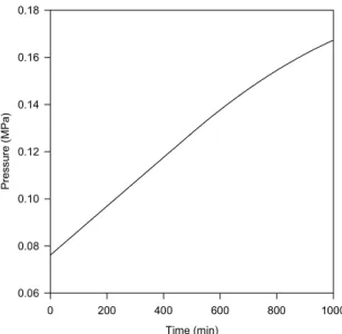
In this example, a new phase appears during the simulation. We consider a tank with a volume of 30 m3 being filled with pure methane. We solve two problems, 1a and 1b, whose specifications are in Table 2. In both cases, the specified heat load corresponds to a heat removal whose rate is time-dependent. Figures 1 and 2 show the evolution of temperature and fluid pressure in the tank in problem 1a. With this set of specifications, there is no condensation of methane in the tank. Figures 3 and 4 present the evolution of the same two variables in problem 1b, showing that both variables pass through a maximum and then decrease after the beginning of heat removal from the tank. At approximately 829 min, there is the onset of a second phase in the tank, what appears in Figs. 3 and 4 as sudden changes in slope.
Table 2: Specifications for example 1.
Problem 1a 1b
Simulation time interval (min) [0, 1000] [0, 1000]
Initial tank temperature (K) 298.15 298.15
Initial mass in the tank (kgmol) 0.9227 0.9227
Initial density (kg/m3) 0.5 0.5
Input stream flowrate (kgmol/min) 0.001 0.01
Input stream temperature (K) 298.15 298.15
Input stream pressure (MPa) 2.0 2.0
Input stream time interval (min) [0, 1000] [0, 1000]
Heat load (kJ/min) −0.01 t( −500) − −(t 500)
Time (min)
0 200 400 600 800 1000
Tem
per
atur
e (K
)
295 300 305 310 315 320 325 330
Time (min)
0 200 400 600 800 1000
P
re
s
su
re
(M
P
a
)
0.06 0.08 0.10 0.12 0.14 0.16 0.18
Figure 1: Temperature evolution in the filling of a tank with methane. Example 1a:
specifications in Table 2).
Figure 2: Pressure evolution in the filling of a tank with methane. (Example 1a:
specifications in Table 2).
Time (min)
0 200 400 600 800 1000
Temp
er
at
ur
e
(
K
)
50 100 150 200 250 300 350 400
Time (min)
0 200 400 600 800 1000
P
re
s
su
re
(M
P
a
)
0.0 0.1 0.2 0.3 0.4 0.5 0.6 0.7
Figure 3: Temperature evolution in the filling of a tank with methane. (Example 1b:
specifications in Table 2).
Figure 4: Pressure evolution in the filling of a tank with methane. (Example 1b:
specifications in Table 2).
Example 2
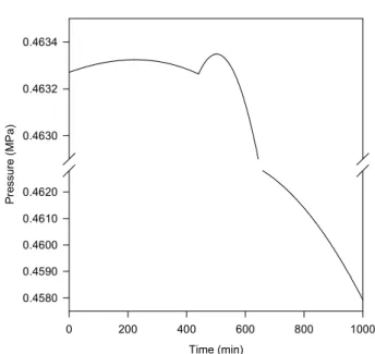
In this example, a phase disappears during the simulation. We consider a mixture of ethane(1) + propene(2) + propane(3) + isobutane(4) + n-butane(5) + n-pentane(6) whose composition is in the range of liquefied petroleum gases (LPG). At the initial condition, presented in Table 3, there are a liquid and a vapor phase in the drum. A vapor stream is continuously withdrawn from the drum and a constant heat load is provided to
282 F. M. Gonçalves, M. Castier and O. Q. F. Araújo
Table 3: Initial conditions for examples 2, 3, and 4.
ethane(1)+propene(2)+propane(3)+iso-butane(4)+n-butane(5)+n-pentane(6)
Tank volume (m3) 4.4232
Initial tank temperature (K) 298.15
Initial mass in the tank (kgmol) 1.0
Initial mole fractions 0.0108; 0.3608; 0.1465; 0.233; 0.233, 0.0159
Table 4: Specifications for example 2.
Simulation time interval (min) [0, 1000]
Output stream flowrate (kgmol/min) 0.0002
Output stream time interval (min) [0, 1000]
Output stream phase vapor
Heat load (kJ/min) 4.0
Heat load time interval (min) [0, 1000]
Time (min)
0 200 400 600 800 1000
Te
mp
era
tur
e (K
)
295 300 305 310 315 320 325 330 335
Time (min)
0 200 400 600 800 1000
P
re
s
s
u
re
(M
P
a
)
0.4580 0.4590 0.4600 0.4610 0.4620 0.4630 0.4632 0.4634
Figure 5: Temperature evolution in the LPG tank (Example 2: specifications in Tables 3 and 4).
Figure 6:Pressure evolution in the LPG tank (Example 2: specifications in Tables 3 and 4). The pressure scale is broken for better visualization of the high-pressure region.
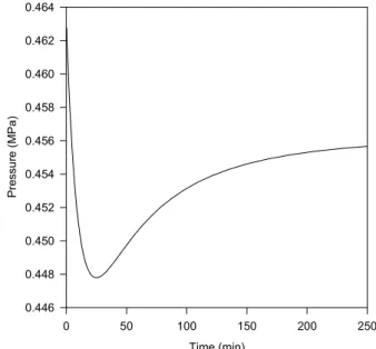
Example 3
We use the same mixture and initial conditions of Example 2, shown in Table 3. In this case, however, there is one input stream and two output streams, corresponding to the withdrawal of the liquid and the vapor phases. The problem specification is presented in Table 5. Given that the flowrate of the output streams is smaller than that of the input stream, material accumulates in the drum. Examining the output specifications, the flowrate of the liquid
Table 5: Specifications for example 3.
ethane(1)+propene(2)+propane(3)+iso-butane(4)+n-butane(5)+n-pentane(6)
Simulation time interval (min) [0, 250]
Input stream flowrate (kgmol/min) 0.120
Input stream temperature (K) 300
Input stream pressure (MPa) 0.6
Input stream mole fractions 0.1667; 0.1667; 0.1667; 0.1667; 0.1667; 0.1667;
Vapor output stream flowrate (kgmol/min) 0.060
Liquid output stream flowrate (kgmol/min) 0.040
Heat load (kJ/min) 0.0
Time (min)
0 50 100 150 200 250
N
u
mb
er of
mol
s
i
n
t
he dr
um (k
g
m
ol
)
0.0 0.2 0.4 0.6 0.8 1.0 1.2 1.4 1.6
ethane propene propane isobutane n-butane n-pentane
Time (min)
0 50 100 150 200 250
Tem
per
at
ur
e (K
)
291 292 293 294 295 296 297 298 299
Figure 7: Evolution of the number of mols in the drum of example 3: specifications in Tables 3 and 5.
Figure 8: Temperature evolution in the drum of example 3: specifications in Tables 3 and 5.
Time (min)
0 50 100 150 200 250
Pr
e
ssu
re
(
M
Pa
)
0.446 0.448 0.450 0.452 0.454 0.456 0.458 0.460 0.462 0.464
284 F. M. Gonçalves, M. Castier and O. Q. F. Araújo
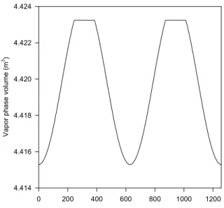
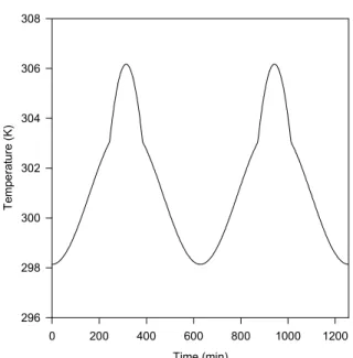
Example 4
In this example, we again use the mixture and initial conditions of Example 2, presented in Table 3. In this example, the tank is closed, but there is a heat load that varies with time according to:
(
)
Q•=sin 0.01t
(8) (t in min and Q in kJ/min)
The system was simulated between 0 min and 400π=1256.64 min, corresponding to two complete disturbance cycles. At the initial condition, there are a liquid and a vapor phase in the drum. Figure 10 shows the evolution of the vapor phase volume. Where a horizontal line represents this volume, there is only the vapor phase in drum. In Figure 11, we show the behavior of the mole fraction of two of the
components, propane and n-pentane, in the liquid phase. Their mole fraction evolutions have opposite patterns because propane is one the lighter components while n-pentane is the heaviest component in the mixture. The interruptions in the lines correspond to the time intervals when there is no liquid phase in the drum. In Figure 12, we show the temperature evolution, in which the discontinuities in the derivative of the temperature with respect to time occur at the points of phase appearance or disappearance. The pressure in the system oscillates between 0.4633 and 0.5155 MPa. This example shows a situation in which there are both phase appearance and disappearance in a single simulation. Given the specified disturbance, which is periodic, it should be expected that the system returned to the initial condition after each complete cycle, which lasts 200π min. This was indeed observed for all variables, showing the consistency of the calculated results.
Time (min)
0 200 400 600 800 1000 1200
V
apor
phase vol
u
m
e
(
m
3)
4.414 4.416 4.418 4.420 4.422 4.424
Figure 10: Evolution of the vapor phase volume in the tank of example 4.
Time (min)
0 200 400 600 800 1000 1200
M
o
le
f
ract
ion
i
n
t
he l
iqui
d phase
0.062 0.064 0.066 0.068 0.070 0.072 0.074 0.076 0.078 0.080 0.082 0.084
propane n-pentane
Time (min)
0 200 400 600 800 1000 1200
Te
mp
era
ture
(K
)
296 298 300 302 304 306 308
Figure 12: Temperature evolution in the tank of example 4.
CONCLUSIONS
The dynamic behavior of flash drums was simulated using a formulation adequate for phase modeling with equations of state (EOS). A new aspect of our dynamic simulations is the use of direct iterations in phase volumes (instead of pressure) for solving the algebraic equations, what has the advantage of avoiding the need for nested loops. It was also observed that an iterative procedure for the UVN flash problem, suggested in the literature, based on the use of logarithms of temperature and phase volumes becomes unreliable close to phase boundaries. We advocate the use of temperature and phase volumes as iterated variables because of the better convergence behavior.
ACKNOWLEDGEMENTS
F.M.G. acknowledges a scholarship from Agência Nacional do Petróleo (ANP, Brazil). The authors are grateful to ANP, CNPq/CTPetro/Brazil, FAPERJ and PRONEX (Contract 124/96) for their financial support.
NOMENCLATURE
Latin Letters
A Helmholtz free energy (-)
ij
f molar flowrate of j
component i in input stream •
f j
H
enthalpy flowrate of inputstream
j
• w k
H
enthalpy flowrate of outputstream
k
i
K
distribution coefficient of componenti
c
n
number of components (-)ij
N number of moles of component i in phase
j
i
N
number of moles of component i in the drum(-)
p
n number of phases (-)
P pressure (-)
•
Q
heat load (-)F
Q
flash function (-)R universal gas constant (-)
f
s
number of input streams (-)w
s
number of output streams (-)t time (-)
T temperature (-)
U internal energy (-)
V drum volume (-)
ik
w
molar flowrate of componenti in output stream
k
Greek Letter
ij
µ chemical potential of component i in phase
286 F. M. Gonçalves, M. Castier and O. Q. F. Araújo
REFERENCES
Castier, M., Automatic Implementation of Thermodynamic Models Using Computer Algebra, Computers and Chemical Engineering, 23, 1229 (1999).
Driedger, W.C., Controlling Vessels and Tanks, Hydrocarbon Processing, 79, No. 3, 101 (2000). Espósito, R.O., Castier, M., and Tavares, F.W.,
Calculations of Thermodynamic Equilibrium in Systems Subject to External Fields, Chem. Engng Sci., 55, 3495 (2000).
Gonçalves, F.M., M.Sc. Thesis, Federal University of Rio de Janeiro, Brazil (2001).
Gopal, V. and Biegler, L.T., Nonsmooth Dynamic Simulation with Linear Programming Based Methods, Computers and Chemical Engineering, 21, 675 (1997).
Michelsen, M.L., The Isothermal Flash Problem. I. Stability Analysis, Fluid Phase Equilibria, 8, 1 (1982a).
Michelsen, M.L., The Isothermal Flash Problem. II. Phase Split Calculations, Fluid Phase Equilibria,
8, 21 (1982b).
Michelsen, M.L., Multiphase Isenthalpic and Isentropic Flash Algorithms, Fluid Phase Equilibria, 33, 13 (1987).
Michelsen, M.L., State Function Based Flash Specifications, Fluid Phase Equilibria, 158-160, 617 (1999).
Müller, D. and Marquardt, W., Dynamic Multiple-Phase Flash Simulation: Global Stability Analysis versus Quick Phase Determination, Computers and Chemical Engineering, 97, S817 (1997). Peng, D.Y. and Robinson, D.B., A New
Two-Constant Equation of State, Ind. Eng. Chem. Fundamentals, 15, 59 (1976).
Press, W.H., Teukolsky, S.A. Vetterling, W.T., and Flannery, B.P., Numerical Recipes in FORTRAN, 2nd ed., Cambridge University Press, Cambridge (1992).
Reid, R.C., Prausnitz, J.M., and Poling, B.E., The Properties of Gases and Liquids, 4th ed., McGraw-Hill, New York (1987).