MULTIOBJECTIVE APPROACH IN PLANS FOR TREATMENT OF CANCER BY RADIOTHERAPY
Thalita Monteiro Obal
1,2*, Neida Maria Patias Volpi
1and Simone Aparecida Miloca
1Received November 21, 2011 / Accepted January 23, 2013
ABSTRACT.Nowadays the technique of radiotherapy has been one of the main alternatives for the treat-ment of several types of cancer today. With technological developtreat-ment, especially in the case of 3D con-formal radiotherapy, applications involving mathematical techniques and algorithms have been proposed to help the development a good treatment plan. This paper aims at present a model for multiobjective linear programming problem of dose intensity. The focus of the model is to determine the best dose distribution of radiation field, so that the dose delivered to the tumor to be prescribed and that affects the minimum the noble and healthy tissues. A test case of prostate cancer was used as an example of the numerical model and the Pareto-Optimal Frontier was generated using the method of weighted function.
Keywords: 3D conformal radiotherapy, multiobjective programming, method of weighted function.
1 INTRODUCTION
The radiotherapy technique is one of the most important alternative for the treatment of cancer nowadays. This type of treatment is based on blocking or destructing the cell division in the DNA molecules that make up the tumor and consisting irradiating the tumor to maximize the effect of radiation on the affected tissues, minimizing adverse impacts on other body tissues. To combat this evil, much has been invested in technology and research.
Most radiotherapy treatment centers in Brazil have modern equipments for radiation emission, the linear accelerators. The equipment has computer systems to support the decision that play a central role in allowing the manipulation of images and the simulation of the effects of a treat-ment regimen.
However, these computer systems can reach quite high costs of implementation and maintenance. Also it do not perform automatic optimization procedures, which is the responsibility of the
*Corresponding author
1Universidade Federal do Paran´a, UFPR, Brazil.
planner’s experience and intuition or by trial and error approach, can generate a solution away from optimal.
The plane of cancer treatment is performed individually but following the same methodology. The treatment plan is carefully developed, based on 3D computed tomography images of the pa-tient, in conjunction with computerized dose calculations to determine the dose intensity pattern that will best conform to the tumor shape. There are three optimization problems relevant to be treated in a treatment plan.
(i) The geometrical problem;
(ii) The problem of dose intensity;
(iii) The problem of the blades opening.
The three problems are the central goal of providing the required dose to eliminate the tumor, with the lowest possible dose to healthy organs (called noble tissues), as well as other body tissues, called healthy tissues.
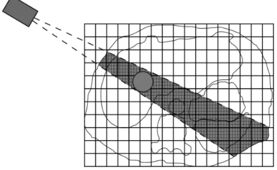
The first problem is to determine the optimal set of directions for each of the radiation beams (Figure 1).
Figure 1– Issuance of a radiation beam. (Source: Goldbarg, 2009).
In Potrebkoet al.(2007), an algorithm to optimize the angle of the radiation beam is proposed, based on minimizing the intersection the amount of the radiation beam in organs at risk. The algorithm was applied for optimization of coplanar beam arrangements regularly spaced in treat-ment of prostate cancer. The authors present a strong correlation between the minimization the amount of the intersection of the radiation beam in the organs at risk with high-dose.
The second problem is the dose intensity and aims at determining the best distribution dose for each radiation beam.
In this regard, Barbozaet al.(2006) use the interior point method to solve the model introduced by Holder (2003). It incorporates elastic constraints that satisfy all constraints for treatment when the solution exists, or has the best solution out of specification, possible to according a weighting of the objective function. Another approach made to the model proposed in Holder (2003) is given by Viana (2010), taking into account the factors of correction for the heterogeneity in the composition of different types of tissue irradiated, based on proportions between their different linear attenuation coefficient.
Also based on the model presented by Holder (2003), Shao (2008) solves the problem of dose intensity through a variant of the method developed by Benson (1998), applying it to a clinical problem in 3D voxel using 5 mm and 3 mm.
The third problem seeks to establish the best opening of the multileaf collimator (Figure 2) taking the shape of the tumor.
Figure 2– Multileaf collimator. (Source: Holder, 2003).
Figure 3– The problem of the sequencing of the blades. (Source: Cambazard, 2009).
Developing a treatment planning is non-trivial. For example, a treatment planner might desire the tumor to receive no less than 80 Gy. Similarly, the planner may hope that some other critical structures receive no more than 40 Gy. So considering that the planner has many options, the use of tools that are capable of generating sets of optimal solutions regarding the impact areas affected by the radiation is helpful.
The problems involved in 3D conformal radiotherapy, from the point of mathematical view, are multiobjective large optimization NP-hard problems (Goldbarg, 2009). The three issues are treated independently in referred literature, because of the complexity of each, which does not exclude the possibility of treating them in an integrated way. Holderet al.(2008), discuss the difficulty of integrating the problems.
This paper proposes a methodology for a dose intensity problem in 3D conformal radiotherapy and a case study is presented as an example of aplication.
2 FORMULATION OF THE PROBLEM OF DOSE INTENSITY
Supposing the existence of a set ofkradiation beams previously defined, the problem is modeled considering a region of the human body obtained from a cut of tomographic image, as shown in Figure 4.
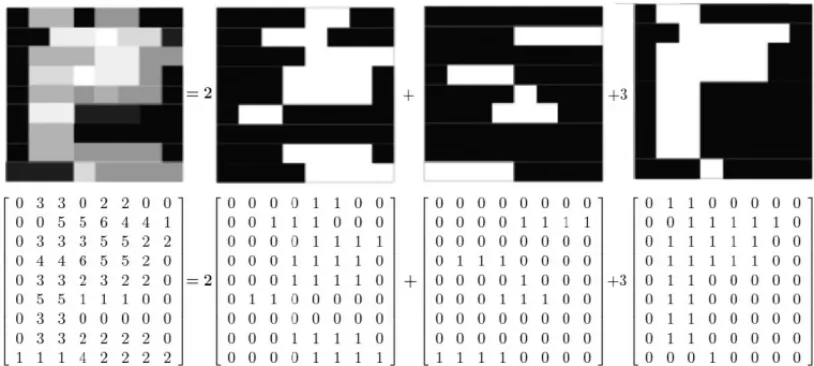
This region is represented by a grid of pixels. Each pixel is considered part of the healthy tissue, tumor, or noble.
Figure 4– Slice of tomographic image of the prostate region. (Source: Erasto Gaertner Hospital, Curitiba/PR.)
This problem is characterized by more than one objective, namely, the concern is not only ra-diating the tumor to maximize the effect of radiation on the affected tissues, but also having a concern as to minimize adverse impacts on other body tissues, so the model can be formulated as a multiobjective optimization model.
2.1 Matrix Absorption Dose
The dose that leaves from each radiation beam is not the same that will reach the tumor. There are several factors that reduce the dose, so that in each region of the body, or better in each pixel, there are different absorption dose. So, it is necessary to construct a matrix that will quantify the absorption dose per pixel, to each unit of radiation emitted by the beam.
LetFk be the matrix of the measure of the factors that influence the energy loss (by radiation beamk, in each pixel(i,j)).
One of the factors included in Fk, for example, is the PDP (Percentage depth dose), which can be measured experimentally. This factor measures the radiation that is received as a function of depth in the dose emitted, whose behavior can be visualized by mean of Figure 5.
LetCkthe matrix that identifies the pixels hit by the beamk, so that:
cki j = (
1 if the pixel(i,j)is affected by the radiation emitted by the fieldk
0 otherwise (1)
Figure 5– Profile of attenuation of the radiation beam with respect to water depth.
heterogeneity in the composition of the irradiated tissue. One way to analyze this absorption is through the shades of gray in tomographic imaging, analyzed in the matrixC T.
Thecti j are values between zero and one, so that the darker the image, this value approaches zero, and the clearer, the value approaches one. Thus, regions of the body clearer in image, such as bone, for example, absorb more energy than the dark regions.
Thus, the matrix that considers all factors of energy absorption is given by:
Ak =C T ⊙Fk⊙Ck (2)
The symbol “⊙” represents the multiplication point-to-point of the elements of the matrices.
LetBn,BsandBtmatrices that associate each pixel as noble, healthy or tumor, respectively.
Bn= (
1 if the pixel(i,j)is noble
0 otherwise (3)
Bs = (
1 if the pixel(i,j)is healthy
0 otherwise (4)
Bt = (
1 if the pixel(i,j)is tumor
0 otherwise (5)
So:
Akn=Ak⊙Bn (6)
Aks =Ak⊙Bs (7)
are the matrices which represent the dose absorption in pixels noble, healthy and tumor, respec-tively, for eachkbeam.
2.2 Objective functions and constraints of the problem
The objective is to determine the amount ofxk dose to be issued for eachkbeam of radiation, restricted to the dose limits for each type of tissue and considering the attenuation suffered by the dose emitted due to several factors. The unit ofxkis the gray(Gy), which is a unit of absorbed dose, defined as the amount you deposit 1 joule (J) of energy per kilogram (kg) from the absorber mean.
The dose determination must be such that the issued dose that reaches to the pixels healthy and noble is the minimum possible and that the tumor dose is the closest to the prescribed by the doctor.
For this, in the model are considered deviations dose per pixels, allowing flexibility in the choice of dose. The matricesθ,δandǫrepresent the deviations of dose and are free variables.
θ=θ+
−θ−
(9)
δ=δ+−δ− (10)
ǫ=ǫ+−ǫ− (11)
The matricesθ+
,δ+
andǫ+
are matrices that represent the deviations of dose in excess in the pixels related to the noble, healthy and tumor, respectively. The matricesθ−
andδ−
represent the dose deviations below the upper limit of the dose of pixels of noble and healthy, respectively, andǫ−is a matrix of deviations dose of tumor deficient in pixels.
The dose that reaches to the noble and healthy pixels must meet the upper dose Sn and Ss, respectively. Then:
( Pm
k=1xkAkn ≤ SnBn
Pm
k=1xkAks ≤ SsBs
(12)
wheremrepresents the number of radiation beams to be used.
Considering that for each pixel can be flexibility in the choice of the absorbed dose, the restric-tions are thus rewritten:
( Pm
k=1xkAkn = SnBn+θ+−θ− Pm
k=1xkAks = SsBs +δ+−δ−
(13)
Moreover,Dis the constant that represents the dose prescribed by the doctor. As the pixels of tumor dose should be givenD, another constraint in the model is in Eq. (14):
m X k=1
Also for the pixels of the tumor, it is considered an absorbed dose of flexibility, represented by the matricesǫ+andǫ−
m X k=1
xkAkt =D Bt +ǫ+−ǫ−. (15)
The model variablesxk,(θi j+),(θi j−),(δ+i j),(δ−i j),(ǫi j+)and(ǫi j−)must all be non-negative.
The objective functions are shown in (16). Two objective functions of the model are to minimize the dose deviation over the pixels of noble and healthy, because they want to get the minimum dose in these pixels. The third and fourth objective are to minimize the dose matrices of devia-tions of excess and lack of tumor dose because the dose that reaches the tumor should be closest to the prescribed by the doctor.
Min f(θ+) = Pl i=1
Pc j=1(θ
+
i j)
Min f(δ+)
= Pli=1Pcj=1(δi j+)
Min f(ǫ+) = Pli=1Pcj=1(ǫi j+)
Min f(ǫ−) = Pl i=1
Pc j=1(ǫ
−
i j)
(16)
wherelandcrepresent the number of rows and columns of the matricesθ+, δ+, ǫ+
andǫ−
.
2.3 Model for implementing the method of weighted function
In the solution of multiobjective problems, two importants aspects are considered: the search for solutions and decision making. For the search of solutions, there is not an optimal solution with respect to all objectives, but rather a set of solutions called efficient solutions (or Pareto-optimal) in which no other solution that is best for all objectives. The image of the Pareto-optimal set is called the Pareto Front. As to the decision, the decision maker is responsible for choosing a particular efficient solution to consider the overall objectives of the problem (Goicoecheaet al.(1982)).
The method used to obtain the Pareto front in the model presented in section 2.2 is the weighted function method, one of the classical methods of multiobjective optimization. This method con-sists in converting the original multiobjective problem into a scalar single-objective problem using different weights for each objective. To obtain Pareto-optimal solutions, we solve the prob-lem iteratively considering different weight vectors (Deb (2009), Goicoecheaet al.(1982)).
Thus, the objective functions are rewritten as shown below.
Min α l X i=1 c X j=1
(θi j+)+β
l X i=1 c X j=1
(δ+i j)+γ1
l X i=1 c X j=1
(ǫi j−)+γ2
l X i=1 c X j=1
(ǫ+i j)
subject to Pm
k=1xkAkn=SnBn+θ+−θ− Pm
k=1xkAks =SsBs+δ+−δ− Pm
k=1xkAkt =D Bt+ǫ+−ǫ−
xk≥0
(θi j+), (θi j−), (δi j+), (δ−i j), (ǫi j+), (ǫ−i j)≥0
(17)
where α, β, γ1 andγ2 represent the weights related to the respective dose deviation matrices
θ+, δ+, ǫ−
andǫ+
.
The solution generated by the model(17)is non-dominated if it satisfy the Theorem 1 (Deb (2009)).
Theorem 1. The solution to the problem presented in (17)is Pareto-optimal if the weights
α, β, γ1andγ2are positive for all objective functions.
3 A CASE STUDY
The test case for numerical example of the model refers to a prostate cancer, whose data were obtained in Erasto Gaertner hospital, Curitiba-PR. This choice is due to being located in a more simplified anatomical region. It was considered a treatment that uses four beams of radiation.
The upper limits for the dose considered noble and healthy tissues, respectively, wereSn=45Gy andSs =50Gy, and the dose to the tumor should reachD=60Gy, usual doses in the treatment of prostate cancer.
The reference image, shown in Figure 4, has been manipulated and exploited by the software MATLAB.
The image initially generated a matrix of order 220×420, determining 554404 variables in the model. Because of computational limitations, it was not possible to work with matrices generated from the original image. Holderet al. (2008) discuss this problem, noting that sometimes it is necessary to reduce the matrices so that problem can be solved. In this study, it was necessary to subject the image to a process of reducing the number of pixels, reducing it to 20% of the previous image.
The grayscale matrixC T, as well as matrices:Ckregarding the incidence in pixeli jforkbundle, Bn which indexes the pixels of tissue noble; Bs which indexes the pixels of healthy tissue; Bt which indexes the pixels of tumor tissue were obtained using the software MATLAB.
Were used tabulated data obtained in dosimetry (Mayleet al.(2007)) for matrix absorption dose
Fk. In this case study, only the factor due to the type of treatment in relation to the distance factor, PDP, was used. Treatment was considered a constant focus-isocenter, held at 600-C linear accelerator with energy of 10 Mev at a distance of 100 cm of the isocenter of the tumor.
4 RESULTS AND DISCUSSION
Using the methodology and model described in section 2.3, the results are presented in Table 1 and were obtained through the toolboxlinprogof MATLAB software.
The average objective function presented in Table 1, is equivalent to the average values of f(ǫ−)
,
f(ǫ+), f(θ+)and f(δ+)on the number of pixels corresponding tissue affected by radiation. For
example:
f(ǫ−)
= f(ǫ
−)
nt wherentis the number of tumor pixels hit by radiation.
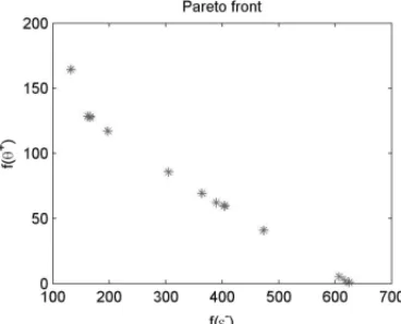
The results presented in Table 1 show that when there is no concern to minimize the deviations of excess dose in healthy and noble pixels, a high dose is applied in some beams and a low-dose in others. This results a greatest dose than the dose limit imposed to the noble and healthy tissues. This solution does not represent a non-dominated solution, because it does not conform to The-orem 1, then is a solution that should be disregarded. The Figures 6 and 7 show the distribution of non-dominated solutions in objective space.
Figure 6– Pareto front in relation to dose deviationsǫ−andθ+.
T H A L IT A MO N T E IR O O B A L , N E ID A MA R IA P A T IA S V O L P I a n d S IMO N E A P A R E C ID A MI L O C A
2
7
γ1 γ2 α β x1 x2 x3 x4 f(ǫ−) f(ǫ+) f(θ+) f(δ+)
P1 1 0 0 0 109.7039 109.6280 140.1498 100.0594 1.2219e-009 3.4659e+003 50.6763 24.1211
P2 0 1 0 0 1.3161 4.8567 4.6371 6.8896 54.6529 0 0 0
P3 0 0 1 0 10.7926 0.0349 11.6881 12.9247 49.6062 0 0 0
P4 0 0 0 1 0.1603 1.7472 2.5477 4.0828 57.6076 0 0 0
P5 0.5 0.5 0 0 54.4269 89.6930 4.8045e-016 9.9455e-017 0.5636 0.5169 14.8319 3.5528
P6 0.4 0.4 0.2 0 17.3744 80.4976 39.3373 28.1150 3.3951 0.4125 0.8512 0.2322
P7 0.4 0.4 0 0.2 60.5773 50.9907 15.7840 30.4235 2.8514 0.3096 5.0160 0.2063
P8 0.4 0.4 0.1 0.1 37.5478 60.9437 35.9878 30.6712 3.3899 0.3908 0.9032 0.2060
P9 0.3 0.3 0.4 0 68.8747 22.7708 42.1343 34.5697 3.9339 0.3504 0.7223 0.1914
P10 0.3 0.3 0 0.4 63.9313 44.7182 18.3010 28.9311 3.6798 0.1470 4.3355 0.1755
P11 0.3 0.3 0.3 0.1 67.6033 24.2277 39.9634 35.0597 4.1554 0.2531 0.7056 0.1794
P12 0.3 0.3 0.1 0.3 66.6019 25.8426 42.7652 30.5836 4.2606 0.2097 0.7050 0.1753
P13 0.3 0.3 0.2 0.2 67.3268 24.7733 44.1715 29.8690 4.2517 0.2182 0.7004 0.1758
P14 0.25 0.25 0.25 0.25 68.4144 23.3654 47.8494 22.9922 5.0633 0.1124 0.6437 0.1532
P15 0.2 0.2 0.6 0 78.7733 9.9827 64.3373 11.9907 5.1078 0.1432 0.6318 0.2008
P16 0.2 0.2 0 0.6 59.9353 46.1792 22.9572 1.0640 10.1861 0 2.8327 0.0249
P17 0.2 0.2 0.5 0.1 73.2687 17.0942 50.1242 11.3779 7.8233 0 0.4706 0.0835
P18 0.2 0.2 0.1 0.5 70.8926 20.5369 37.0683 11.9095 10.3679 0 0.3295 0.0303
P19 0.2 0.2 0.4 0.2 75.9312 13.7474 51.2077 5.2288 9.3459 0 0.3806 0.0495
P20 0.2 0.2 0.2 0.4 72.1020 18.8968 37.6440 12.1391 10.3598 0 0.3261 0.0306
P21 0.2 0.2 0.3 0.3 78.5208 10.4020 42.1033 12.9537 9.9900 0 0.3421 0.0380
P22 0.1 0.1 0.8 0 83.6732 1.8472 25.6281 10.1361 16.0629 0 0.0035 0.0025
P23 0.1 0.1 0 0.8 53.3256 50.2442 18.3116 5.2461 11.3233 0 1.6471 0.0131
P24 0.1 0.1 0.7 0.1 79.2771 9.1462 18.5660 12.2285 16.0182 0 0.0050 0.0020
P25 0.1 0.1 0.1 0.7 38.9925 56.2469 18.1007 15.3094 12.3598 0 0.2637 0.0101
P26 0.1 0.1 0.6 0.2 79.2771 9.1462 18.5660 12.2285 16.0182 0 0.0050 0.0020
P27 0.1 0.1 0.2 0.6 70.5604 20.5931 22.3041 19.7125 12.1363 0 0.2242 0.0129
P28 0.1 0.1 0.5 0.3 79.2771 9.1462 18.5660 12.2285 16.0182 0 0.0050 0.0020
P29 0.1 0.1 0.3 0.5 70.8703 20.1927 27.9829 3.5040e-011 15.5739 0 0.0292 0.0022
P30 0.1 0.1 0.4 0.4 79.2771 9.1462 31.6278 8.9232e-015 15.8402 0 0.0127 0.0023
As for conflicting objectives, note that the closer the dose to be applied is the prescribed dose, or f(ǫ−)near zero, which is desirable for the tumor, greater is the deviation in the tissues noble
and healthy, a result which is not desired for such tissue.
Although the methodology presented does not indicate a single optimal solution, but a set of compromise solutions, shown in Pareto frontier (Figures 6 and 7), the decision on which one is chosen as the final solution, it is the specialist decision maker, due to other clinical criteria. To help this choice, this paper suggested following criteria: the solution chosen is the one with the smallest euclidean distance in relation to the ideal point.
The ideal point is that whose coordinates are formed by the best solution for each objective (Deb (2009)). The Figure 8 shows the representation of the ideal point in relation to the solutions of the Pareto frontier, which has coordinates(f(ǫ−),
f(θ+), f(δ+))
=(3,3899;0,0050;0,0020).
Figure 8– Best solution in relation to ideal point.
According to the criterion used, the “best solution” was found was f(ǫ−)=3.3899, f(θ+)=
0.9032 and f(δ+)=
0.2060, with weights for each functions areγ1=0.4, α=0.1 andβ =0.1,
and the values of doses issued by each beams radiation is x1 = 37,54780, x2 = 60,94370, x3=35,98780 andx4=30,6712.
5 CONCLUSIONS
allow comparisons between the results generated with different weight vectors. Pareto’s front showed the importance of the decision maker in multiobjective problems. Observing that in con-flicting situations it is necessary to penalize some factors to winning in others. It is proposed a criterion for the decision of choice.
ACKNOWLEDGMENTS
The authors would like to thank the team of radiotherapy of Erasto Gaertner Hospital, Curitiba – Paran´a, with the number 2042 project approved by the Ethics Committee on Research. Thalita Monteiro Obal acknowledges the support of CAPES through scholarship REUNI.
REFERENCES
[1] ACOSTA R, BRICK W, HANNA A, HOLDER A, LARA D, MCQUILEN G, NEVIN D, UHLIGP & SALTER B. 2008. Radiotherapy optimal design: An Academic Radiotherapy Treatement Design System, Matematics Faculty Research.
[2] ARAUJO FS. 2010. Um estudo algor´ıtmico para otimizac¸˜ao do plano de tratamento em radioterapia conformal, Dissertac¸˜ao de Mestrado, Universidade Federal do Rio Grande do Norte, Natal.
[3] BARBOZA CB & OLIVEIRA AR. 2006. Planejamento do tratamento por radioterapia atrav´es de m´etodos de pontos interiores.Pesquisa Operacional,26(1): 1–24.
[4] BENSON HP. 1998. Anouter approximation algorithm for generating all eficient extreme
points in the out come set of a multiple objective linear programming problem.Journal of Global Optimization,13: 1–24.
[5] CAMBAZARD H, O’MAHONY E & O’SULLIVAN B. 2009. A Shortest Path-based Ap-proach to the Multileaf Collimator Sequencing Problem.Integration of AI and OR
Tech-niques in Constraint Programming of Combinatorial,5574: 41–55.
[6] DEBK. 2009. Multi-objective optimization using evolutionary algorithms. Wiley.
[7] GOICOECHEAA, HANSENDR & DUCKSTEINL. 1982. Multiobjetive decision analysis with engineering and business applications. John Wiley & Sons.
[8] GOLDBARGMC. 2009. Algoritmo evolucion´ario para otimizac¸˜ao do plano de tratamento em radioterapia conformal 3D.Pesquisa Operacional,29(2): 239–267.
[9] HOLDERA. 2003. Designing radiotherapy plans with elastic constraints and interior point methods.Healt Care Management Science,6: 5–16.
[10] MAYLES P, NAHUM A & ROSENWALD JC. 2007. Handbook of radiotherapy physics.
Taylor & Francis Group, LLC.
[12] SHAOL. 2008. Multiple Objective Linear Programming in Radiotherapy Treatment Plan-ning. Thesis of doctory, Department of Engineering Science, School of Engineering, Uni-versity of Auckland.