doi: 10.1590/0101-7438.2016.036.01.0167
COMPARISON OF MIP MODELS FOR THE INTEGRATED LOT-SIZING AND ONE-DIMENSIONAL CUTTING STOCK PROBLEM
Gislaine Mara Melega
1*, Silvio Alexandre de Araujo
1and Raf Jans
2Received November 30, 2015 / Accepted April 1, 2016
ABSTRACT.Production processes comprising both the lot-sizing problem and the cutting stock problem are frequent in various industrial sectors. However these problems are usually treated separately, which can generates suboptimal overall solution and consequently causes production losses. In this paper, we propose different mathematical models for the integrated problem combining alternative models for the lot-sizing and the cutting stock problem, in order to evaluate and indicate the impact of these changes on the models’ performance. An extensive computational study is done using randomly generated data and as a solution strategy we used a commercial optimization package and the application of a column generation technique.
Keywords: Capacitated Lot-Sizing Problems, One-Dimensional Cutting Stock Problem, Column Genera-tion.
1 INTRODUCTION
Technological advances and increasing competition in industries have become worldwide phe-nomena. Some prominent aspects of these advances are the emphasis on knowledge and the development of new technologies. Inserted on this context, mathematical models that describe and improve the production processes have been studied and used as tools to support decision making in the business environment. Among the various decision processes, this work is part of the tactical/operational planning of production with the lot-sizing problem and cutting stock problem. The Lot-Sizing Problem (LSP) considers the tradeoff between the setup and inventory costs to determine at minimal cost the size of production lots to meet the demand of each final product, while the cutting stock problem (CSP) involves the cutting of large objects into smaller items, so as to minimize the total loss of material.
The literature mostly deals with these two problems separately. However, in industrial sectors such as furniture, paper and aluminum, the lot-sizing and cutting stock problems are found in
*Corresponding author.
1Departamento de Matem´atica Aplicada, IBILCE, UNESP – Universidade Estadual Paulista, 15054-000 S˜ao Jos´e do Rio Preto, SP, Brasil. E-mails: [email protected]; [email protected]
consecutive phases. For these cases, a decoupled vision of the problems usually used by com-panies, can provide good local solutions but, at the end of planning processes, these solutions may conflict with the global objectives and feasibility of production. This fact was observed in Gramani et al. (2009) in the furniture industry. In this case, solutions generated from the lot-sizing problem can lead to infeasible solutions for the cutting stock problem with regard to the production capacity of the cutting machine. If, on the other hand, for a given period, the pro-duction exceeds demand, this circumstance may generate cutting patterns with less loss, and a decrease of setup costs. However, there is an increase of inventory costs and physical space for allocation of items to be stored will be needed, which may not exist in practice. For this reason, the relevance of these issues in the industrial sectors and the benefits in dealing with problems in an integrated way makes this an appropriate research topic today. Motivated by this, the present paper proposes mathematical models and solution methods for solving the integrated lot-sizing and cutting stock problem.
In this work, the capacitated lot-sizing problem is modeled using the mathematical model pro-posed by Trigeiro et al. (1989), denoted here byCL. We also considered the variable redefinition strategy (Eppen & Martin, 1987) which reformulates the lot-sizing problem as a shortest path problem. This reformulation is called SP. The idea of this variable redefinition was originally proposed for uncapacitated problems and Jans & Degraeve (2004), Jans (2009), Fiorotto & de Araujo (2014) and Melega et al. (2013) extended this to cases with capacity constraints, related parallel machines, unrelated parallel machines and various plants, respectively. More informa-tion on reformulainforma-tion for lot-sizing problems can be found in Denizel et al. (2008), which shows several theoretical and computational results between some reformulations.
To model the one-dimensional cutting stock problem, we consider three mathematical models from the literature. The first one is the model developed by Kantorovich (1960), here denoted byKT. This model is also called the generalized assignment formulation forCSP(Degraeve & Peeters, 2003) and determines the best way to cut objects to meet the demand, minimizing the number of objects used. For this model, an upper bound on the number of objects is considered. The second model dealt with, and perhaps the best known among the academic community, is the one proposed by Gilmore & Gomory (1961, 1963) denoted here byGG. This model produces good lower bounds when compared to theKTmodel, however it has an large number of variables, which indicates the use of column generation to deal with this difficulty.
The third model was proposed by Val´erio de Carvalho (1999, 2002), here denotedVC. The au-thors propose an alternative mathematical model for the one-dimensional cutting stock problem based on an arc flow problem. Thus, finding a valid cutting pattern for the cutting stock problem is equivalent to finding a path in a directed acyclic graph. The authors also consider additional con-straints to guarantee that demand is satisfied. This model is efficient in the sense that it presents a linear relaxation as good as the Gilmore and Gomory model.
multi-objects). In a second part of this study, these models are integrated into the uncapacitated lot-sizing problem proposed by Wagner & Whitin (1958), here calledWW.
Next, in Section 2, there is a literature review with the major studies that address the lot-sizing and the cutting stock problem in an integrated way. The Sections 3, 4 and 5 describe the proposed integrated models with capacity constraints, several object types and a reformulation for the lot-sizing, respectively. In Section 6, the solution strategies are described. The computational results are presented in Section 7. And finally, the conclusions are presented in Section 8.
2 LITERATURE REVIEW
The importance of addressing the problems in an integrated way has become increasingly ev-ident in the literature and is closely related to industrial applications. Possibly Farley (1988) had been the first paper that treats these problems in an integrated way. The author addressed the problem in an clothing industry, where the problem involves irregular two-dimensional cuts. Hendry et al. (1996) conducted a case study on a copper components factory. The objective was to investigate alternative methods of generating production plans for casting in order to minimize costs and meet demand. Non˚as & Thorstenson (2000, 2008) studied the problem coupled with the addition of setup cost in a Norwegian company that produces off-road trucks. The company needed a production plan that minimizes the total cost in the cutting process and in the produc-tion line. Therefore, the authors proposed a model and different soluproduc-tion methods. Gramani & Franc¸a (2006) formulated a mathematical model for the integrated problem in a furniture industry and proposed a solution method based on an analogy with the shortest path problem. Compu-tational results compared the proposed method to the method used in the industry. Poltroniere et al. (2008) studied the integrated problem applied to the paper industry. The authors analyzed the production process and proposed a mathematical model for machines operating in paral-lel and presented two heuristics based on Lagrangian relaxation considering the problems in a decoupled way.
model for the integrated problem in the context of a furniture factory. The authors considered the cutting patterns used by industry and n-groups cutting pattern to solve the problem with a set of real data provided by the factory. An extension to Gramani et al. (2011) model was proposed in Vanzela et al. (2013) in order to simulate the practice of a small furniture factory.
Alem & Morabito (2012) used robust optimization tools to solve the integrated problem in the furniture industry, where the production costs and demand of products are uncertain parame-ters. Computational tests were performed using real and simulated data. Le˜ao & Arenales (2012) studied a simplification of the model studied in Poltroniere et al. (2008). Two approaches have been studied: (i) for a single type of object and (ii) for various types of objects. Three mathemat-ical models for each approach have been proposed and they used the column generation as the solution method. To obtain a feasible solution, the columns obtained with the column generation method are used and the resulting integer problem with this limited set of columns is solved.
Silva et al. (2014) presented two integer programming models for the integrated problem. In these models, both the bringing forward of items for production and also the stocking of reusable leftovers for the cutting process in later periods were allowed. The authors proposed two heuris-tics and evaluated the models through a computational study, checking the quality of the so-lutions when compared to work described in the literature. In more recent papers, Poldi & de Araujo (2016) studied the multi-period cutting stock problem and Molina et al. (2016) proposed an integrated lot sizing and packing problem that is related to the problem studied in this paper.
Most of the studies in the literature that address the integrated lot-sizing and cutting stock prob-lem study several cases of the probprob-lem in practice. In these studies, alternative formulations for theLSPandCSPare not tested in order to choose the formulation that best fits the problem and the data set. So, extending the ideas of Longhi et al. (2015) this paper tries to cover the gap by proposing alternative mathematical formulations, considering different features of the lot-sizing and cutting stock problem such as capacity constraints and several object types. Furthermore, through the use of extensive computational tests, it intends to evaluate and point out the impact of these changes in the performance of the models.
3 MATHEMATICAL MODELS WITH CAPACITY CONSTRAINT
In this section the lot-sizing problem proposed by Trigeiro et al. (1989) (CLmodel) is integrated with various cutting stock formulations as described above. The integrated lot-sizing and cutting stock model is a two level production model, with production of final products at the final level, and the cutting of the pieces at the preceding level. The proposed model assumes that final prod-ucts can be kept in inventory, but pieces cannot be kept in inventory. Furthermore, the Bill of Material indicates that one final product requires exactly one piece, and each type of final prod-uct requires a different piece. Therefore, there is a one-to-one relationship between final prodprod-ucts and pieces in the model.
for example) which creates demand for subassemblies or components (a door, for example) (Gramani & Franc¸a, 2006). After the cutting process, the cut items pass through another produc-tive process (e.g. drilling and painting) before being ready to be assembled into a final product. Usually these other productive processes are considered the bottlenecks of the complete pro-duction process (Ghidini et al., 2007; Santos et al., 2011; Alem & Morabito, 2013), and their capacity is considered in the model, whereas the final assembly is not considered in the model since it is not a bottleneck process. Ghidini et al. (2007) and Alem & Morabito (2013) considered the drill machine capacity in terms of items. Santos et al. (2011) considered aggregated capac-ity constraints for all the other machines (except the cutting machine). For the one-dimensional case, considered in this paper, the same type of capacity constraints appear. For instance, in tubular furniture industries, the bending machine is a bottleneck of the production process and its capacity must be considered in the mathematical model.
A second potential practical background appears in industries where the cut items are directly transformed in end items, i.e., there is no need to assemble several items to compose a final product, but there is a production process between the cut items and the end items. The capac-ity constraint in terms of end items means that the capaccapac-ity constraints are related to the final production process to transform the cut items into the final items.
Consider the following parameters and decision variables:
Parameters:
T: number of time periods (indext);
I: number of items (indexi);
scit: setup cost of itemiin periodt; hcit: unit holding cost of itemiin periodt; stit: setup time of itemiin periodt; vtit: production time of itemiin periodt; capt: capacity (in unit of time) in periodt; dit: demand of itemiin periodt;
sditr: sum of demand of itemifrom periodtuntil periodr; L: object length;
li: length of itemi; co: fixed cost of an object.
Decision Variables:
Xit: production quantity of itemiin periodt;
Sit: inventory for itemi at the end of periodt;Yit: binary variable indicating the production or
not of itemi in periodt.
Q: number of objects available in stock (indexq);
yqt: binary variable that indicates whether objectqis used in periodt; hiqt: variable that indicates the amount of itemicut from objectqin periodt.
ModelCLKT
min
T
t=1 I
i=1
(scitYit +hcitSit)+ T
t=1 Q
q=1
coyqt (1)
Subject to:
Xit +Si,t−1=dit+Sit ∀i, ∀t (2)
Xit ≤sdit TYit ∀i, ∀t (3)
I
i=1
(stitYit+vtitXit)≤Capt ∀t (4)
I
i=1
lihiqt ≤L yqt ∀q, ∀t (5)
Q
q=1
hiqt =Xit ∀i, ∀t (6)
Yit, yqt∈ {0,1} ∀i, ∀q, ∀t (7)
hiqt ∈Z+ ∀i, ∀q, ∀t (8)
Xit, Sit ∈R+ ∀i, ∀t (9)
The objective function (1) minimizes the machine setup costs, inventory holding costs and the cost of cutting objects. Constraints (2) are the demand constraints: inventory carried over from the previous period and production in the current period are available to be used to satisfy current demand and build up inventory. Constraints (3) force the setup variable to one if any production takes place in that period. Next, there is a constraint on the available capacity in each period (4). Constraints (5) are from the cutting stock problem and ensure that if objectqis used, the com-bination of the lengths of items that will be cut from it should not exceed its length. Constraints (6) are responsible for the integration of the lot-sizing and cut stock problem decision, that is, we have to cut a sufficient amount of items to meet the planned production amount. Finally, the set of constraints (7), (8) and (9) define the non-negativity and integrality conditions. It is known that the modelKT for the cutting stock problem has a weak linear relaxation and presents many symmetric solution (Val´erio de Carvalho, 2002).
Observe that the variables Xit and constraints (6) could be eliminated by replacing Xit by
Q
q=1hiqt in the rest of the model. However to compare this model with other proposed models,
the variableXit and the constraints (6) are kept explicitly in the model. This remark is also valid
The second integrated formulation presented below (CLVC) uses theVCmodel for the cutting stock problem, which is modeled as an arc flow problem. Consider a path in a directed acyclic graphG = (V,A), withV = {0,1, . . . ,L}and the set of arcs of the graph defined as A = {(j,l);0≤ j <l <L and l− j =li for all i ≤ I}. The losses in the object generated from
the cutting process are represented in the graph by additional arcs between the vertices(j,j+1)
to j=0, . . . ,L−1. As decision variables for the integrated modelCLVCwe have:
ft: flow through the network in periodt;
zjlt: number of cutting patterns which have an item of size(l−j)allocated at a distance jfrom
the beginning of the object in periodt.
ModelCLVC
min
T
t=1 I
i=1
(scitYit+hcitSit)+ T
t=1
co ft (10)
Subject to:
Xit+Si,t−1=dit+Sit ∀i, ∀t (11)
Xit ≤sdit TYit ∀i, ∀t (12)
I
i=1
(stitYit +vtitXit)≤Capt ∀t (13)
−
(0,l)∈A
z0lt = −ft ∀t (14)
(g,l)∈A zglt−
(l,h)∈A
zlht=0 l =1, . . . ,L−1,∀t (15)
(l,L)∈A
zl Lt = ft ∀t (16)
(h,h+li)∈A
zh,h+li,t =Xit ∀i, ∀t (17)
Yit ∈ {0,1} ∀i, ∀t (18)
zlht, ft ∈Z+ ∀(l,h)∈ A, ∀t (19)
Xit, Sit ∈R+ ∀i, ∀t (20)
The objective function (10) minimizes the machine setup and inventory costs of the items, as well as the cost of the flow through the network. The flow set for this problem represents the number of used objects (cutting patterns), since one flow unit defines a path, which in turn defines a cutting pattern.
characteris-tic of the Val´erio de Carvalho model. Constraints (17) integrate the two problems and constraints (18), (19) and (20) are non-negativity and integrality constraints.
This model also presents many symmetric solutions, or alternatives that correspond to the same cutting patterns. For this reason, Val´erio de Carvalho (1999) presented some reduction criteria to eliminate some arcs, reducing the number of symmetric solutions without eliminating any valid cutting patterns from set A. This study applies the criterion consisting of allocating the items in order of decreasing length in each cutting pattern, that is, an item of lengthi1 can only be placed after another item lengthi2ifi1≤i2, or at the beginning of the object. Another criterion also used does not allow starting with a cutting pattern with loss. Thus, the first arc of loss will be inserted in the graph at a distance from the beginning of the object representing the shortest item length.
The third model CLGG combines the lot-sizing model CL with the cutting stock model GG
(Gilmore & Gomory, 1961, 1963), which has the following parameters and decision variables:
J: set of cutting patterns (index j);
ai j: parameter indicating the quantity of itemicut according to the cutting pattern j; xj t: variable indicating the number of objects cut according to cutting pattern jin periodt.
ModelCLGG
min
T
t=1 I
i=1
(scitYit+hcitSit)+ T
t=1
j∈J
coxj t (21)
Subject to:
Xit+Si,t−1=dit +Sit ∀i, ∀t (22)
Xit ≤sdit TYit ∀i, ∀t (23)
I
i=1
(stitYit +vtitXit)≤Capt ∀t (24)
j∈J
ai jxj t =Xit ∀i, ∀t (25)
Yit ∈ {0,1} ∀i, ∀t (26)
xj t ∈Z+ ∀j, ∀t (27)
Xit, Sit ∈R+ ∀i, ∀t (28)
(Val´erio de Carvalho, 2002). As a consequence this model has a large amount of variables and is generally solved by column generation.
4 MATHEMATICAL MODELS WITH SEVERAL TYPES OF OBJECTS
For the mathematical models presented in this section, we integrate the model proposed by Wagner & Whitin (1958), here denoted byWWwith the cutting stock models extended to con-sider several types of objects. TheWW model describes the uncapacitated lot-sizing problem. In this case, consider the following parameters and additional decision variables:
Parameters:
K: number of object types available in stock (indexk);
ekt: planned supply of object typekat the beginning of periodt; Lk: object length of typek;
cw: cost per unit of raw material waste.
Decision Variable:
skt: number of objects of typekstocked at end of periodt.
The model described below (WWKTMO) models the cutting stock problem based on modelKT, considering several types of objectsMO. In the original variables a new index is inserted, which refers to the type of object to be cut.
Parameters:
sekt: sum of planned supply of objects of typekfrom period 1 to periodtsekt =ta=1eka; q ∈ {1, . . . ,sekt}, index for the available objects.
Decision Variables:
yqkt: binary variable that indicates whether objectqof typekis used in periodt; hiqkt: quantity of itemicut from objectqof typekin periodt.
ModelWWKTMO
min
T
t=1 I
i=1
(scitYit +hcitSit)+cw
⎛
⎝
T
t=1 K
k=1 sekt
q=1
Lkyqkt− T
t=1 K
k=1 sekt
q=1 I
i=1 lihiqkt
⎞
⎠ (29)
Subject to:
Xit+Si,t−1=dit +Sit ∀i, ∀t (30)
Xit ≤sdit TYit ∀i, ∀t (31)
I
i=1
lihiqkt ≤ Lkyqkt ∀q, ∀k, ∀t (32)
K
k=1 sekt
q=1
ekt +sk,t−1= sekt
q=1
yqkt+skt ∀k, ∀t (34)
Yit, yqkt ∈ {0,1} ∀q, ∀i, ∀k, ∀t (35)
hiqkt ∈Z+ ∀q, ∀i, ∀k, ∀t (36)
Xit, Sit,skt ∈R+ ∀i, ∀t (37)
The objective function (29) minimizes machine setup costs, inventory holding costs and waste cost in the cutting process. Constraints (30) and (31) refer to the lot-sizing problem and are defined as in the CLKT model. The set of constraints (32) ensure that if an object q of type
k is used, the combination of the items that will be cut from it should not exceed its length. Constraint (33) is responsible for the integration of the decision variables of the lot-sizing and cutting stock problems. It ensures that a sufficient amount of items are cut to meet the demand. The set of constraints (34) ensure that the number of objects cut in each period does not exceed the availability in stock.
The integrated model presented below (WWVCMO), is based on theVCformulation to model the cutting stock problem. Since several object types are available in stock, we need to define the maximum object lengthLmax = max∀k{Lk}, corresponding to the numbers of nodes in the
network. The following decision variables are also needed:
fkt: flow through the network in the periodtfor the object typek;
zjlt: number of cutting patterns which have a item of size(l−j)allocated at a distance j from
the beginning of the object used in periodt.
ModelWWVCMO
min
T
t=1 I
i=1
(scitYit+hcitSit)+cw
⎛
⎝
T
t=1 K
k=1
Lkfkt− T
t=1 I
i=1
(l,l+li)∈A
lizl,l+li,t
⎞
⎠ (38)
Subject to:
Xit +Si,t−1=dit+Sit ∀i, ∀t (39)
Xit ≤sdit TYit ∀i, ∀t (40)
−
(0,l)∈A
z0lt = − K
k=1
fkt ∀t (41)
(g,l)∈A zglt−
(l,h)∈A
zlht=0 l= {1, . . . ,Lmax−1}\ K
a=1
{La}, ∀t (42)
(g,Lk)∈A
zg Lkt = fkt ∀k, ∀t (43)
(h,h+li)∈A
ekt+sk,t−1= fkt +skt ∀k, ∀t (45)
Yit ∈ {0,1} ∀i, ∀t (46)
zglt, fkt ∈Z+ ∀(g,l)∈ A, ∀k, ∀t (47)
Xit, Sit ∈R+ ∀i, ∀t (48)
The objective function (38) minimizes machine setup costs and storage costs of the items, and waste cost of raw material. Constraints (39) and (40) are defined as in theCLKT model. The set of constraints (41), (42) and (43) correspond to the flow conservation constraints. Constraints (44) integrate the cutting stock and lot-sizing problem. Constraints (45) ensure that the stock of the different types of available objects is respected and constraints (46), (47) and (48) are non-negativity and integrality constraints.
The following formulation (WWGGMO) models the cutting stock problem proposed by Gilmore & Gomory (1961) with an extension for several objects, which has the following parameters and decision variables. Observe that an index that refers to the type of object is also needed.
Parameters:
Jk: set of cutting patterns that use object typek(index j);
aik j: quantity of itemicut from object typekaccording to cutting pattern j.
Decision Variable:
xk j t: number of objects of typekcut using cutting pattern jin periodt.
ModelWWGGMO
min
T
t=1 I
i=1
(scitYit +hcitSit)+cw
⎛
⎝
T
t=1 K
k=1
j∈Jk
Lkxk j t− T
t=1 K
k=1
j∈Jk I
i=1
liaik jxk j t
⎞
⎠
(49)
Subject to:
Xit+Si,t−1=dit +Sit ∀i, ∀t (50)
Xit ≤sdit TYit ∀i, ∀t (51)
K
k=1
j∈Jk
aik jxk j t =Xit ∀i, ∀t (52)
ekt+sk,t−1=
j∈Jk
xk j t+skt ∀k, ∀t (53)
Yit ∈ {0,1} ∀i, ∀t (54)
xk j t ∈Z+ ∀k, ∀j, ∀t (55)
The objective function (49) minimizes machine setup cost and inventory cost of items, and costs of waste due to the cutting of objects. Constraints (50) and (51) refer to the lot-sizing problem. The set of constraints (52) is responsible for the integration of the decision variables of the two problems. The constraints (53) ensure that the number of cut objects in each period does not exceed the availability in stock, and the constraints (54), (55) and (56) are non-negativity and integrality constraints.
5 INTEGRATED MODELS USING THE REFORMULATED LOT-SIZING PROBLEM
SP
The integrated models presented in Sections 3 and 4 use the classical formulation for the lot-sizing problem. In order to obtain better lower bounds, the lot-lot-sizing problem is reformulated as a shortest path problem (Eppen & Martin, 1987) and then integrated into the respective cut-ting stock problem. For that, we need the following definitions of parameters and variables, respectively:
cvitr: inventory holding cost of itemi in periodt at a quantity that meets the demands for the
periods fromtuntilr;
zvitr: fraction of the production plan for itemito satisfy demand from periodtto periodr.
The lot-sizing problem variables have the following correspondence:
Xit = T
r=t
sditrzvitr ∀i, ∀t (57)
and the demand constraints (2) and setup constraints (3) are rewritten in terms of the new decision variables as follows:
T
r=1
zvi1r =1 ∀i (58)
t−1
r=1
zvirt−1= T
r=t
zvitr ∀i, ∀t\{1} (59)
T
r=t
zvitr ≤Yit ∀i, ∀t (60)
Constraints (58) and (59) define the flow constraints in theSPmodel. For each itemi, a unit flow is sent through the network (constraint (58)), imposing that its demand has to be satisfied without backlogging in each period (59)). Constraint (60)) ensures that itemiwill be produced in periodt only if there is a setup prepared to produce that item.
Thus, we propose new mathematical models that integrate the cutting stock problems (KT, VC, GG, KTMO, VCMO, GGMO) into the reformulated lot-sizing problem (SP). This is done by replacing the decision variables in the models, by the new variables and constraints described above.
As an example, the integrated modelSPKTis shown next.
ModelSPKT
min
T
t=1 I
i=1
scitYit + T
r=t
cvitrzvitr
+
T
t=1 Q
q=1
coyqt (61)
Sujeito a:
T
r=1
zvi1r =1 ∀i (62)
t−1
r=1
zvirt−1= T
r=t
zvitr ∀i, ∀t\{1} (63)
T
r=t
zvitr ≤Yit ∀i, ∀t (64)
I
i=1
stitYit + T
r=t
vtitsditrzvitr
≤Capt ∀t (65)
I
i=1
lihiqt ≤L yqt ∀q, ∀t (66)
Q
q=1 hiqt =
T
r=t
sditrzvitr ∀i, ∀t (67)
Yit, yqt∈ {0,1} ∀i, ∀q, ∀t (68)
hiqt ∈Z+ ∀i, ∀q, ∀t (69)
zvitr, Sit ∈R+ ∀i, ∀t (70)
The objective function (61) minimizes the setup costs and inventory holding costs according to theSPmodel, as well as, the cost of the number of objects to be cut. The constraints (62) and (63) define the flow constraints of theSPmodel. The set of constraints (64) also refers to the model
6 SOLUTION STRATEGIES
Two heuristic strategies are proposed for solving the models described in sections 3, 4 and 5. The first heuristic consists of solving the models integrated withKTandVCusing a commercial optimization package with a stopping criteria. The solver is stopped at the end of 600 seconds or when the gap between the upper bound and lower bound is less than 0.1%. The second heuristic proposes the search for a feasible solution by using the column generation technique for the models integrated withVCandGG. The solver is used to solve the restricted master problems, the sub-problems and also to solve the resulting integer restricted master problem.
Next, the column generation based heuristic is explained in more detail together with the proce-dure to obtain a feasible solution.
6.1 Initial Basic Solution
Considering the model with capacity constraint and integrated with theGGmodel, the master problem starts with the columns related to the homogeneous cutting pattern, i.e., columns of type:(0, . . . ,aii, . . . ,0), whereaii = ⌊lLi⌋, ∀i. The same columns are inserted for each period, t =1, . . . ,T.
For the problems with several objects, the master problem starts with homogeneous cutting pat-terns generated for each object type, i e., for each objectkcolumns of type(0, . . . ,aiki, . . . ,0),
whereaiki = ⌊Llik⌋, ∀i, are inserted in order to avoid the infeasibility of an initial basic solution.
The same columns are inserted for all periods. Similar ideas are applied to the models integrated withVC.
6.2 Column Generation Procedure
The sub-problems in the column generation consist of finding a new cutting pattern for the master problem. For the models integrated withGG, the sub-problem is composed of the knapsack constraint and for those integrated withVCthe sub-problem is composed of the flow constraints imposing a flow equal to one, which represents a cutting pattern.
Considering the models with one type of object and a capacity constraint, a sub-problem is solved for every period, and the column with the smallest reduced cost over all periods is included in the master problem. As a consequence, the same column is also inserted for each period. For the problems with several objects, a sub-problem is solved for each period and object type, and the column with the smallest reduced cost is inserted into the master problem. The same column is used for all periods according to the corresponding object in the restricted master problem.
6.3 Feasibility Strategy
all the columns obtained in the column generation procedure is solved using the optimization package with a time limit of 600 seconds and an optimality gap of 0.1%.
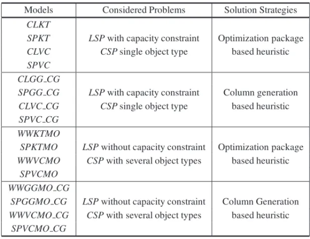
Table 1 presents a summary of all proposed mathematical models and solution strategies.
Table 1– Mathematical Models and Solution Strategies.
Models Considered Problems Solution Strategies
CLKT
SPKT LSPwith capacity constraint Optimization package
CLVC CSPsingle object type based heuristic
SPVC CLGG CG
SPGG CG LSPwith capacity constraint Column generation
CLVC CG CSPsingle object type based heuristic
SPVC CG WWKTMO
SPKTMO LSPwithout capacity constraint Optimization package
WWVCMO CSPwith several object types based heuristic
SPVCMO WWGGMO CG
SPGGMO CG LSPwithout capacity constraint Column Generation
WWVCMO CG CSPwith several object types based heuristic
SPVCMO CG
7 COMPUTATIONAL STUDY
This section presents the computational results used to evaluate and compare the performance of the proposed models. The analysis of the results is done through tables containing the aver-age values found by models with respect to different aspects, as well as the use of the perfor-mance profile technique (Dolan & Mor´e, 2002). This technique provides a tool which facilitates the exhibition and the interpretation of comparisons and it is briefly described in the following paragraphs.
ConsiderPas the set ofᒋpinstances andMas the set ofᒋMmodels described in sections 3, 4 and 5. The values obtained for each instance (upper bound and gap)p ∈Pusing them∈Mmodel is denoted byvp,m. For each modelm∈Ma comparison of its performance on the instancep ∈P
relative to the performance of the best model is given by the following performance ratio:
rp,m =
vp,m
minm∈M{vp,m} .
If the modelmdoes not find a feasible solution for an instance p thenrp,m is defined asrM,
feasible instances in all the models. The performance of the model m compared to the other models is given by the performance profile:
ρm(τ )=
1
ᒋp|{p∈P: rp,m ≤τ}|
with |.| representing the number of elements in the set. The performance profile ρm(τ ) is a
function that is associated to a given valueτ ∈R, and indicates the fraction of instances solved by the modelmwith a performance within a factorτ of the best performance found. With this, each model has a curve that shows its performance for each levelτ. Due to the fact thatrM can
be considerably large, the logarithm scale is used to represent the performance profile. It is done as follows (Dolan and Mor´e, 2002):
τ → 1
ᒋp
|{p∈P:log2(rp,m)≤τ}|.
This way, theτ factor varies in[0,rM), withrM =1+max{log2(rp,m): p∈Pandm∈M}.
The models are written in the AMPL syntax (Fourer et al., 1990) and CPLEX 12.5 (IBM, 2009) is used as solver. All the computational tests are conducted on a 2.93GHz Intel Core i7 processor with 8GB of RAM memory.
7.1 Experiment 1
Next, we describe the data generation and computational results for the integrated problem with capacity constraints (models in Section 3 and the corresponding models in Section 5). In this experiment we present two sets of data: the first one called Data 1, is based on a data generator for the cutting stock problem. The second set, referred to as Data 2, is based on some examples widely used in the literature to solve the lot-sizing problem.
7.1.1 Data Sets
For the Data 1 set, the CUTGEN1 generator proposed by Gau & W¨ascher (1995) is used and for the lot-sizing problem the data set is based on Trigeiro et al. (1989). The parameters are generated in intervals[a,b]with a uniform distribution as follows:
• number of periods:T =15
• object length:L=1000
• number of items: I= {10,20,40}
• length of items are generated in three intervals according toli ∈ [v1, v2], with v1 =
0.01Lor 0.2L andv2=0.02Lor 0.8L
• raw material cost:co=1;
• setup cost:scit ∈ [100,500]
• inventory cost:hcit ∈ [1,5]
• production time:vtit =1
• setup time:stit ∈ [10,50]
• capacity (capt) is generated by the average of lot-by-lot policies: for every periodt
cal-culate the amount of resources needed to produce exactly the demands of the items in this period, sum up this amount for all periods and divide by the number of periodsT, this is,
capt = T
t=1Ii=1(vtitdit+stit)
T .
In the cutting stock problem modeled byKT, an upper bound on the number of objects in stock (Q) is needed. Poldi & Arenales (2010) is the basis for calculating the upper bound asQ=2⌈λ⌉
with,λ=
T
t=1Ii=1lidit
L .
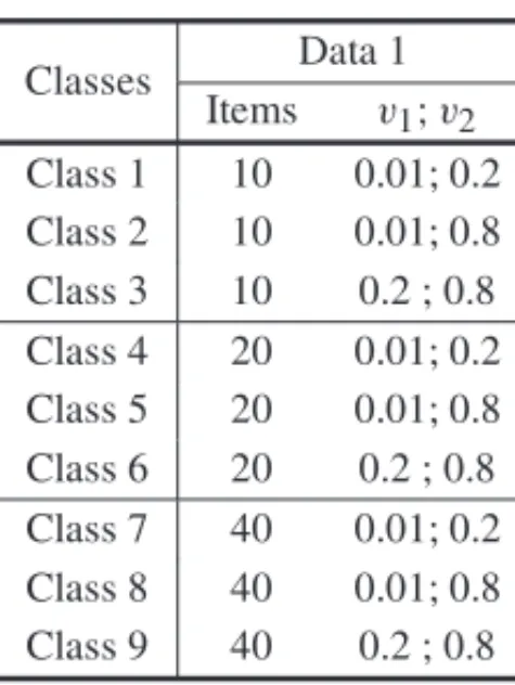
Thus, the Data 1 defines 9 classes (see Table 2), and for each class 10 random instances are generated considering the three levels of capacity, totaling 270 instances.
Table 2– Classes of Data 1.
Classes Data 1
Items v1;v2
Class 1 10 0.01; 0.2
Class 2 10 0.01; 0.8
Class 3 10 0.2 ; 0.8
Class 4 20 0.01; 0.2
Class 5 20 0.01; 0.8
Class 6 20 0.2 ; 0.8
Class 7 40 0.01; 0.2
Class 8 40 0.01; 0.8
Class 9 40 0.2 ; 0.8
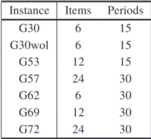
The second data set, called Data 2, is based on the lot-sizing problem. This set is created using 7 specific instances from Trigeiro et al. (1989) (see Table 3). These instances are considered difficult and have been used in several studies in the literature (Jans & Degraeve, 2004; Vyve & Wolsey, 2006; Degraeve & Jans, 2007; de Araujo et al., 2015).
Table 3– Specific Instances and Classes of Data 2.
Instance Items Periods
G30 6 15
G30wol 6 15
G53 12 15
G57 24 30
G62 6 30
G69 12 30
G72 24 30
Classes Data 2
v1;v2 Class 10 0.01; 0.2 Class 11 0.01; 0.8 Class 12 0.2 ; 0.8
7.1.2 Computational Results
Firstly, we present the computational results using Data 1.
A preliminary test is performed in order to evaluate the impact of the models and the capacity tightness on the number of feasible solutions found. It is considered three different levels of capacity: cap0 where we have the integrated problem without capacity constraint;cap1 where the value of the capacity iscapt/0.3;cap2 where we have tighter capacity given bycapt/0.85.
The results shown that the number of feasible solutions decreases as the capacity becomes more scarce. TheCLVCmodel is the only formulation able to find feasible solutions for all instances, but only for the uncapacitated case. The CLVCmodel obtained the largest number of feasible solutions for the three capacity levels using the optimization package based heuristic. For the column generation based heuristic the best performance in this analysis is obtained byCLVC CG
model. In general, the difficulty to find a feasible solution is in Classes 4 and 7, which correspond to classes in which the ratio between the item length and object length is small.
The following results are evaluated considering the uncapacitated model (columncap0) and with
capt/0.3 (columncap1).
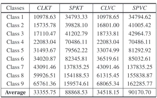
In Table 4 the lower bound obtained with the linear relaxation for the models is presented. As a general conclusion, regarding the cutting stock problem, the models integrated withVC,VC CG
andGG CGare equivalent with relation to the value of the lower bound obtained. For this reason just one of them is presented and the lower bounds are better than the lower bounds resulting from the models integrated withKT. The value obtained withcap0 andcap1 are the same for all the models and just one value is presented. Regarding the lot sizing problem the models integrated withSPobtain a substantially better lower bound than the models usingCL.
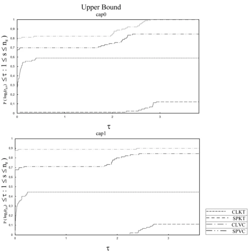
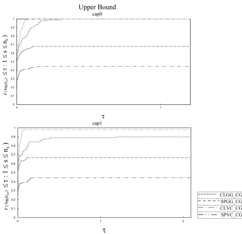
Figures 1 and 2 show the performance profiles obtained with the upper bound for all the instances in Data 1. Considering the optimization package based heuristic (see Fig. 1), theCLVCmodel shows a good overall performance in both variations of capacity, since its performance profile dominated the rest of them. This model could find the best upper bound for around 70% of the in-stances, followed by theSPVC. For the column generation based heuristic (see Fig. 2),CLVC CG
Table 4– LP Relaxation for Data 1.
Classes CLKT SPKT CLVC SPVC
Class 1 10978.63 34793.33 10978.65 34794.62
Class 2 15735.78 39828.10 16801.00 41005.42
Class 3 17110.47 41202.79 18733.81 42964.73
Class 4 22083.04 70486.11 22083.04 70486.11
Class 5 31493.67 79562.22 33074.99 81292.92
Class 6 34020.87 82345.81 36519.61 85032.61
Class 7 43091.46 137835.25 43091.46 137835.25
Class 8 59926.51 154188.53 61315.45 155838.87
Class 9 65761.36 159574.61 68065.34 162285.77
Average 33355.75 88868.53 34518.15 90170.70
considering thecap0 instances it is possible to obtain an upper bound for all the instances with theCLVC,CLVC CGandCLGG CGmodels. The lowest number of feasible solutions, around 10% and 40%, are found respectively by theSPKTandSPVC CGmodels. In general, mathemat-ical models integrated intoVCobtained the best results for most instances in both the capacity variations and heuristic strategies.
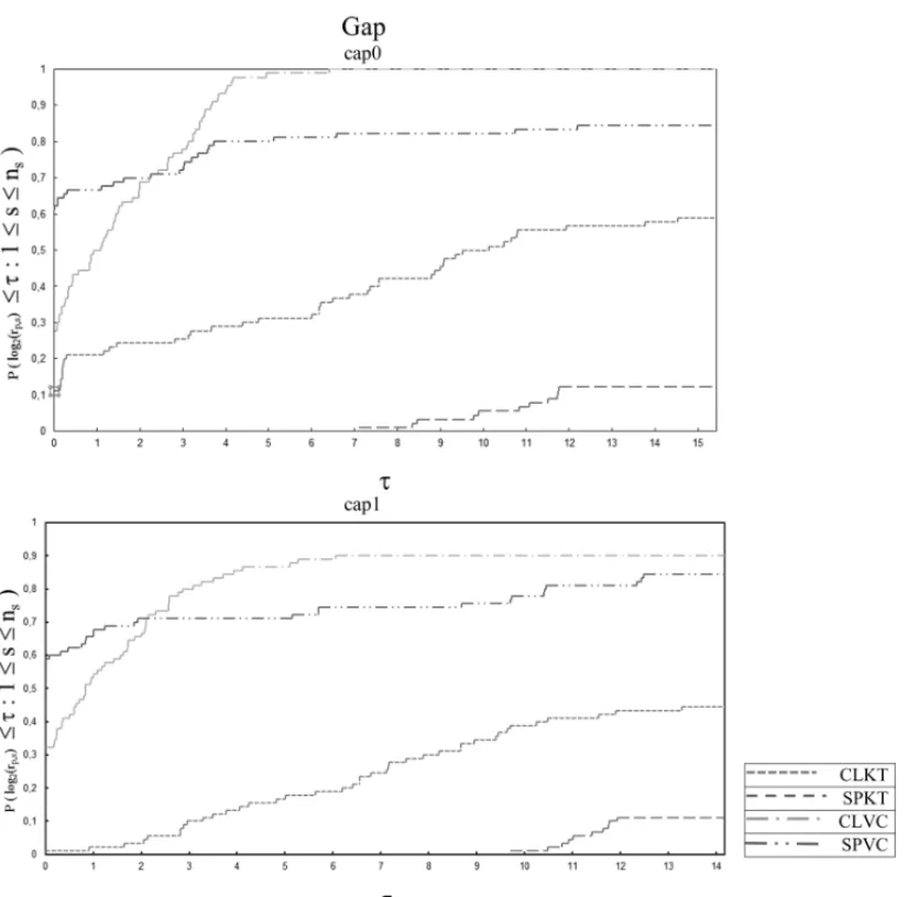
Figure 3 shows the performance profile obtained for the gap for models solved with the opti-mization package based heuristic. The gap is that provided by the solver for the final solution for both the cases cap0 and cap1. In both variations of capacity, theSPKT could not find a satisfactory results for the gap. TheCLVCmodel showed a good overall performance, in which 100% and 90% of the instances obtained a feasible solution forcap0 andcap1, although it has the best performance in just 30% of the instances. On the other hand, theSPVCmodel showed the best performance in approximately 60% of the instances, but with the disadvantage of not having solved all the instances. Since the column generation procedure is subject to a time limit, we cannot guarantee the optimality of this lower bound, and therefore no results on the gap are presented for theCGmethods.
The computational results for Data 2 are given as follow.
The same analysis for Data 2 is performed in order to evaluate the impact of the models and the capacity tightness on the number of feasible solutions found. It is noticed a big difficulty of theSPKT model to solve these instances. TheSPVC CGmodel also shows great difficulties in finding a feasible solution. Class 12 presents the largest number of feasible solutions (378 from 560), followed by Class 11 (369 from 560). In Class 12, half of the models found a feasible solution for all the instances; this class is related with the longest items when compared to object length.
Figure 1– Performance Profiles: Upper Bound for the Optimization Package Based Heuristic – Data 1.
to the models integrated with the classical lot-zing model. This improvement is 260% on average. The models integrated withKTdid not achieve a value for the linear relaxation for some instances within a time of 5 hours.
Figure 4 shows the performance profile of the upper bound and gap considering the optimization package based heuristic. The first impact observed in the figure is due to the huge difference between the models integrated withKTandVCto obtain an upper bound. TheSPKTandCLKT
models found an upper bound for around just 5% and 40% of the instances, respectively. On the other hand, theSPVCandCLVCmodels found a upper bound for around 65% and 90% of the instances, respectively. The best performance to obtain the upper bounds is found using the
Figure 2– Performance Profiles: Upper Bound for the Column Generation Based Heuristic – Data 1.
which reached at most 10% of the best results (atτ =0). The performance obtained with the
SPVCmodels changes a little when the gap is analyzed. The performance of theSPVCbecomes around the same asCLVC, 40% of the best results (τ =0). And one more time, results obtained withCLVCmodel dominate the other models considering the performance values (τ).
Figure 3– Performance Profiles: Gap for Optimization Package Based Heuristic – Data 1.
7.2 Experiment 2
The following describes the generation of data and computational results for the integrated un-capacitated lot-sizing and the cutting stock problem with several types of objects (the models in Section 4 and its corresponding model in Section 5).
7.2.1 Data Set
Table 5– LP Relaxation for Data 2.
Class 10 CLKT SPKT CLVC SPVC
Example 1 12552.56 38450.41 12552.81 38455.10
Example 2 12534.92 38645.79 12535.19 38649.20
Example 3 25058.61 74650.39 25058.67 74651.33
Example 4 46554.59 143706.15 46554.59 143706.16
Example 5 13311.81 63092.75 13312.38 63096.81
Example 6 30428.71 136060.92 30428.72 136062.38
Example 7 64483.84 299427.41 64483.84 299427.59
Average 29275.01 113433.40 29275.17 113435.51
Class 11
Example 1 14831.41 40729.26 15257.52 41292.36
Example 2 14813.77 40924.64 15243.59 41476.43
Example 3 29619.41 79211.19 30346.19 80104.87
Example 4 56385.07 153536.63 57257.32 154658.84
Example 5 18060.64 67841.58 18919.93 68835.03
Example 6 40162.36 145794.58 41623.78 147495.46
Example 7 — — 86738.85 322311.95
Average — — 37912.46 122310.71
Class 12
Example 1 15702.19 41600.04 16508.34 42542.73
Example 2 15684.55 41795.42 16493.35 42720.26
Example 3 31270.20 80861.98 32472.08 82150.89
Example 4 59625.74 156777.30 61617.88 158934.87
Example 5 19827.17 69608.12 21501.31 71404.10
Example 6 43685.89 149318.11 46154.93 152056.45
Example 7 — — 95674.65 331111.52
Average — — 41488.93 125845.83
(−)time limit with no lower bound
• number of periods:T = {3,6}
• types of objects: K = {3,5}
• number of items: I = {10,20}
• object length:Lk ∈ [300,1000]
• planned supply of object typekin periodt:ekt ∈ [1.5⌈λt⌉,2⌈λt⌉]with,λt = I
i=1lidit K
k=1Lk .
• item length:li ∈ [0,1L,0,4L], whithL = K
k=1Lk K
Figure 4– Performance Profiles: Upper Bound for the Optimization Package Based Heuristic – Data 2.
• raw material cost:cw=1;
• setup cost:scit ∈ [100,500]
• inventory cost:hcit ∈ [1,5]
Thus, the data set defines 8 classes (see Table 6), and for each class 10 random instances are generated, totalling 80 instances.
7.2.2 Computational Results
Figure 5– Performance Profiles: Upper Bound for the Column Generation Based Heuristic – Data 2.
Table 6– Classes with several types of objects.
Classes Periods Objects Items
Class 13 3 3 10
Class 14 3 3 20
Class 15 3 5 10
Class 16 3 5 20
Class 17 6 3 10
Class 18 6 3 20
Class 19 6 5 10
Class 20 6 5 20
Table 7 presents the computational results obtained for the lower bound. The use of the refor-mulated lot-sizing model shows significant improvements in the lower bound. A slight improve-ments can be seen in the use ofVCmodel when compared with theKTmodel.
Tables 8 and 9 show the average upper bounds in each class for each mathematical model. TheWWKTMOandSPKTMO models did not find a feasible solution for most classes. Con-sidering the optimization package based heuristic theWWVCMOmodel found the best results for almost all the classes (except Classe 16). For the column generation based heuristic the best results are shared betweenWWGGMO CGandSPGGMO CGmodels. As theWWGGMO CG
model obtained results which are very close to the best found, this fact contributed to the best global average. Note thatWWVCMOperforms very poorly on Class 20, compared to the column generation methods. This is also confirmed by the largest gap for this class.
Table 7– LP Relaxation.
Classes WWKTMO WWVCMO SPKTMO SPVCMO
Class 13 4861.68 4861.68 5472.80 5472.80
Class 14 9840.43 9840.43 9931.05 9931.05
Class 15 4801.52 4868.99 5201.06 5201.06
Class 16 9872.04 9873.19 9872.04 9873.19
Class 17 6831.39 6831.39 8743.99 8779.76
Class 18 13455.68 13455.68 13510.54 13510.54
Class 19 6584.89 6584.89 7436.32 7436.32
Class 20 13626.16 13637.07 13626.16 13637.07
Average 8734.22 9225.75 8742.66 9230.23
Table 8– Upper Bounds for the Optimization Package Based Heuristic.
Classes WWKTMO WWVCMO SPKTMO SPVCMO
Class 13 18014.40 8081.20 40179.80 8081.70
Class 14 (*5) 15188.20 — 15214.40
Class 15 17307.50 7629.40 30391.60 7629.90
Class 16 (*6) 14634.00 — 14627.67
Class 17 (*4) 16447.10 — 16507.30
Class 18 (*2) 28801.30 — 29546.30
Class 19 (*5) 15560.80 — 15721.90
Class 20 — 219048.63 — (*1)
Average — 40673.83 — —
(−)time limit with no integer solution
(∗)number of instances with feasible solution
Table 9– Upper Bounds for the Column Generation Based Heuristic.
Classes WWGGMO CG WWVCMO CG SPGGMO CG SPVCMO CG
Class 13 8171.40 8509.50 8161.40 8456.80
Class 14 15440.90 20884.90 15442.40 21045.90
Class 15 7586.40 9196.00 7577.20 9373.10
Class 16 14941.00 22470.22 14999.89 22707.78
Class 17 16616.10 19200.20 16675.70 19736.20
Class 18 29996.20 47068.00 33889.80 51973.40
Class 19 15335.90 19712.30 15334.60 20369.80
Class 20 32340.50 45904.88 52861.25 47941.50
Average 17553.55 24118.25 20617.78 25200.56
Table 10– Final Gap.
Classes WWKTMO WWVCMO SPKTMO SPVCMO
Classe 13 58.79 0.10 80.41 0.11
Classe 14 (*5) 0.29 — 0.46
Classe 15 58.94 0.08 74.78 0.08
Classe 16 (*6) 0.39 — 0.35
Classe 17 (*4) 0.24 — 0.22
Classe 18 (*2) 2.78 — 3.96
Classe 19 (*5) 0.50 — 1.55
Classe 20 — 48.16 — (*1)
Average — 6.57 — —
8 CONCLUSIONS
In this paper, we present a study of mathematical models from the literature for modeling the lot-sizing problem and the one-dimensional cutting stock problem, in order to propose and compare new integrated problems. For the lot-sizing problem, we study the model proposed by Wagner & Whitin (1958), the model proposed by Trigeiro et al. (1989) and a reformulation of the lot-sizing problem proposed by Eppen & Martin (1987). For the cutting stock problem, extensions of the models proposed by Kantorovich (1960), Val´erio de Carvalho (1999, 2002) with reduction criteria and Gilmore & Gomory (1961) have been proposed to incorporate multiple periods. These models have been extended also to consider various types of objects.
In the literature, there are several studies of practical cases, which use these formulations to model the problems found, as simple or integrated problems. This study aims to present alter-native mathematical models for the integrated problem in order to compare and point out the advantages of each model, as well as, the impact of the data set on the obtained solutions. As solution methods, we present two strategies. The first one uses a solver for finding the solution. In the second one, the column generation technique is used in a heuristic strategy to get a feasible solution. An extensive computational study is conducted with different data sets.
The difficulty of the models to obtain a feasible solution becomes clear when considering the capacity constraint in the lot-sizing problem, and this impact is even greater when the capacity constraint is tight. The main influence of the data set on the results is in instances that have an item length considerably smaller when compared to the object length. For the models that consider various object types in stock, the main impact of the data in the results comes from the increase in the number of items.
constraints, the classical lot-sizing model integrated with the Val´erio de Carvalho model and Gilmore and Gomory in both capacity variations (uncapacitated model andcapt = capt/0,3)
obtained a lot of good upper bounds. However the use of the shortest path model (Eppen & Martin, 1987) significantly improved theLPlower bound and obtained gaps smaller when com-pared to other models, for most classes. In an analysis for the mathematical models with various object types, although the integration with the Gilmore and Gomory model does not show the best results for all classes for the upper bound, the proximity to the best results contributes to the achievement of best overall average.
A possible direction for future research is to study other extensions of the models proposed and develop more elaborate solution methods, in order to address a greater variety of instances.
ACKNOWLEDGEMENTS
We would like to thank the anonymous referees for their constructive comments, which led to a clearer presentation of the material. This research was funded by the Conselho Nacional de Desenvolvimento Cient´ıfico e Tecnol´ogico – CNPq and the Fundac¸˜ao de Amparo a Pesquisa do Estado de S˜ao Paulo – FAPESP (process no. 474782/2013-1, 2012/20631-2, 2014/17273-2 and 2014/01203-5).
REFERENCES
[1] ALEMD & MORABITOR. 2013. Risk-averse two-stage stochastic programs in furniture plants.OR Spectrum,35(4): 773–806, 2013. ISSN 0171-6468.
[2] ALEMDJ & MORABITOR. 2012. Production planning in furniture settings via robust optimization.
Computers & Operations Research,39(2): 139–150.
[3] DEARAUJOSA,DEREYCKB, DEGRAEVEZ, FRAGKOSI & JANSR. 2015. Period decompositions for the capacitated lot sizing problem with setup times.INFORMS Journal on Computing, 27(3): 431–448.
[4] DEGRAEVEZ & JANSR. 2007. A new dantzig-wolfe reformulation and branch-and-price algorithm for the capacitated lot-sizing problem with setup times.Operations Research,55(5): 909–920. [5] DEGRAEVEZ & PEETERSM. 2003. Optimal integer solutions to industrial cutting-stock problems:
Part 2, benchmark results.INFORMS Journal on Computing,15(1): 58–81.
[6] DENIZELM, ALTEKINFT, S ¨URALH & STADTLERH. 2008. Equivalence of the lp relaxations of two strong formulations for the capacitated lot-sizing problem with setup times.OR Spectrum,30(4): 773–785.
[7] DOLAN ED & MOR´EJJ. 2002. Benchmarking optimization software with performance profiles.
Mathematical Programming,91(2): 201–213.
[8] EPPENGD & MARTINRK. 1987. Solving multi-item capacitated lot-sizing problems using variable redefinition.Operations Research,35(6): 832–848.
[10] FIOROTTODJ &DE ARAUJOSA. 2014. Reformulation and a lagrangian heuristic for lot sizing problem on parallel machines.Annals of Operations Research,217(1): 213–231.
[11] FOURERR, GAYDM & KERNIGHANBW. 1990. A modeling language for mathematical program-ming.Management Science,36(5): 519–554.
[12] GAU T & W ¨ASCHER G. 1995. Cutgen1: A problem generator for the standard one-dimensional cutting stock problem.European Journal of Operational Research,84(3): 572–579.
[13] GHIDINI CTLS & ARENALES MN. 2009. Otimizac¸˜ao de processos acoplados na ind´ustria de m´oveis: dimensionamento de lotes e corte de estoque. InAnais do CNMAC-Congresso Nacional de Matem´atica Aplicada e Computacional.
[14] GHIDINICTLS, ALEMD & ARENALESMN. 2007. Solving a combined cutting stock and lot-sizing problem in small furniture industries. InProceedings of the 6th International Conference on Operational Research for Development (VI-ICORD).
[15] GILMOREPC & GOMORYRE. 1961. A linear programming approach to the cutting-stock problem.
Operations Research,9(6): 849–859.
[16] GILMOREPC & GOMORYRE. 1963. A linear programming approach to the cutting stock problema – part ii.Operations Research,11(6): 863–888.
[17] GRAMANIMCN & FRANC¸APM. 2006. The combined cutting stock and lot-sizing problem in in-dustrial processes.European Journal of Operational Research,174(1): 509–521.
[18] GRAMANIMCN, FRANC¸APM & ARENALESMN. 2009. A lagrangian relaxation approach to a coupled lot-sizing and cutting stock problem.International Journal of Production Economics,119(2): 219–227.
[19] GRAMANIMCN, FRANC¸APM & ARENALES MN. 2011. A linear optimization approach to the combined production planning model.Journal of the Franklin Institute,348(7): 1523–1536. [20] HENDRYLC, FOKKK & SHEKKW. 1996. A cutting stock and scheduling problem in the copper
industry.The Journal of the Operational Research Society,47(1): 38–47.
[21] IBM CORPORATION. 2009. CPLEX. http://www-01.ibm.com/software/integration/optimization/ cplex-optimizer/, 2009. visitada pela ´ultima vez em 12/10/2012.
[22] JANSR. 2009. Solving lot-sizing problems on parallel identical machines using symmetry-breaking constraints.INFORMS Journal on Computing,21(1): 123–136.
[23] JANSR & DEGRAEVEZ. 2004. Improved lower bounds for the capacitated lot sizing problem with setup times.Operations Research Letters,32(2): 185–195.
[24] KANTOROVICHLV. 1960. Mathematical methods of organizing and planning production. Manage-ment Science,6(4): 366–422.
[25] LEAO˜ APS & ARENALESMN. 2012. An´alise de modelos matem´aticos para o problema de corte de estoque unidimensional acoplado ao dimensionamento de lotes. InAnais do XLIV SBPO-Simp´osio Brasileiro de Pesquisa Operacional, Rio de Janeiro-RJ.
[27] MELEGAGM, FIOROTTODJ & DE ARAUJOSA. 2013. Formulac¸˜oes fortes para o problema de dimensionamento de lotes com v´arias plantas.TEMA (S˜ao Carlos),14: 305–318. ISSN 2179-8451. [28] MOLINAF, MORABITOR &DEARAUJOSA. 2016. Mip models for production lot-sizing problems
with distribution costs and cargo arrangement.Journal of the Operational Research Society. Accept to Publication.
[29] NONAS˚ SL & THORSTENSONA. 2000. A combined cutting-stock and lot-sizing problem.European Journal of Operational Research,120(2): 327–342.
[30] NONAS˚ SL & THORSTENSONA. 2008. Solving a combined cutting-stock and lot-sizing problem with a column generating procedure.Computers & Operations Research,35(10): 3371–3392. [31] POCHETY & WOLSEYLA. 2006.Production planning by mixed integer programming. Springer
Science & Business Media.
[32] POLDIKC & ARENALESMN. 2010. O problema de corte de estoque unidimensional multiper´ıodo.
Pesquisa Operacional,30: 153–174.
[33] POLDIKC &DE ARAUJOSA. 2016. Mathematical models and a heuristic method for the multi-period one-dimensional cutting stock problem.Annals of Operations Research,238(1): 497–520. [34] POLTRONIERESC, POLDIKC, TOLEDOFMB & ARENALESMN. 2008. A coupling cutting
stock-lot sizing problem in the paper industry.Annals of Operations Research,157(1): 91–104.
[35] SANTOSSG,DEARAUJOSA & RANGELMSN. 2011. Integrated cutting machine programming and lot sizing in furniture industry.Pesquisa Operacional para o desenvolvimento,3(1): 1–17. [36] SILVAE, ALVELOSF & VALERIO DE´ CARVALHOJM. 2014. Integrating two-dimensional cutting
stock and lot-sizing problems.Journal of the Operational Research Society,65(1): 108–123. [37] TRIGEIRO WW, THOMAS LJ & MCCLAIN JO. 1989. Capacitated lot sizing with setup times.
Management Science,35(3): 353–366.
[38] VALERIO DE´ CARVALHOJM. 1999. Exact solution of bin-packing problems using column genera-tion and branch-and-bound.Annals of Operations Research,86: 629–659.
[39] VALERIO DE´ CARVALHOJM. 2002. Lp models for bin packing and cutting stock problems.European Journal of Operational Research,141(2): 253–273.
[40] VANZELAM, RANGELS &DE ARAUJOSA. 2013. The integrated lot sizing and cutting stock problem in a furniture factory. InIntelligent Manufacturing Systems, volume 11, pages 390–395. [41] VYVE MV & WOLSEYLA. 2006. Approximate extended formulations.Mathematical
Program-ming,105(2-3): 501–522.