ISSN 0101-8205 www.scielo.br/cam
Nonlinear cutting stock problem model to minimize
the number of different patterns and objects
ANTONIO CARLOS MORETTI1 and LUIZ LEDUÍNO DE SALLES NETO2 1Instituto de Matemática, Estatística e Computação Científica – UNICAMP
Cidade Universitária Zeferino Vaz s/n, Barão Geraldo, 13084-790 Campinas, SP, Brazil
2Escola de Engenharia Industrial Metalúrgica – UFF
Av. dos Trabalhadores, 420, Vila, 27255-970 Volta Redonda, RJ, Brazil E-mails: [email protected] / [email protected]
Abstract. In this article we solve a nonlinear cutting stock problem which represents a cutting stock problem that considers the minimization of, both, the number of objects used and setup. We use a linearization of the nonlinear objective function to make possible the generation of good columns with the Gilmore and Gomory procedure. Each time a new column is added to the problem, we solve the original nonlinear problem by an Augmented Lagrangian method. This process is repeated until no more profitable columns is generated by Gilmore and Gomory technique. Finally, we apply a simple heuristic to obtain an integral solution for the original nonlinear integer problem.
Mathematical subject classification: 65K05.
Key words: cutting problem, nonlinear programming, column generation.
1 Introduction
The Unidimensional Cutting Stock Problem (1/V/I/R according Dyckhoff [5]) is characterized by cutting stocks in just one dimension. More specifically, we havemitems with different sizes with width equal towiand we must cut, through its length, a minimum number of master rolls (with widthW > wi for alli) to attend demanddi for each itemi. Each combination of items cut from a master
roll is called a cutting pattern. The problem is to determine the frequency of each cutting pattern to attend demand and (for instance) minimize the number of objects cut.
A reasonable goal to be met in a industry is to minimize the number of master rolls used to produce the demanded items. If we consider that there are a suffi-cient number of objects of same widthW available, then the formulation below describes the mathematical model that minimize the total number of objects (i.e., master rolls) used in a cutting plan:
(P1)
Minimize c1 n j=1 xj subject to n j=1
ai jxj ≥di, i =1, . . . ,m. xj ∈N, j =1, . . . ,n. where
• c1is the cost for each master roll used;
• ai j is the number of itemsiin cutting pattern j;
• xj is the number of of objects cut according cutting pattern j.
In some cases, the minimization the number of objects used are not the only goal for the manager. In fact, when we have a large demand to attend in a short period of time, the number of machine setup done for cutting the items from the master rolls takes a growing importance, since each time we process a cutting pattern there is a need to adjust the knives in the cutting machine and this adjustment takes time. Adding this setup cost in the previous problem (P1) we obtain a new formulation which minimizes the number of objects and the number of setup:
(P1)
Minimize c1 n j=1
xj +c2 n
j=1 δ(xj)
subject to n
j=1
wherec2is the setup cost andδ(xj)=
1 ifxj >0, 0 ifxj =0.
Combinatorial problems involving setup costs are known to be very hard to solve. In particular (P1) presents two conflicting objectives: (1) Minimize the total number of processed objects and (2) the total number of setup used.
Solving problem (P1) is already a hard task to do, since it is a N P-Hard prob-lem. Problem (P1) is a harder problem, since, besides being a nonlinear integer problem, the nonlinear part of the objective function is discontinuous. This fact, does not allow us to solve the problem by using the Gilmore and Gomory strategy [9, 10]. Vanderbeck [22] investigates the problem of minimizing the number of different cutting patterns as an integer nonlinear programming, where the number of objects is fixed. In his approach, Vanderbeck uses Dantzig-Wolfe decomposition [20, 21]. Since the model considered works with a huge number of variables, the method solves only problems with a small number of items. For this reason several papers considering this problem involve the use of heuristic procedures. Below, we describe two of these methods which will be used to compare with our approach.
• Sequential Heuristic Procedure – SHP: It was proposed by Haessler [11] and it is based on an exaustive technique of cutting pattern repetitions. In each iteration an aspiration criterion is computed then a search is done to look for cutting patterns that satisfy such parameters until the demand are all attended. The SHP give us a good initial solution and it is used by others method to compare the quality of their solutions. It generates an inexpensive good initial solution to the (P1).
Kombi can be seen as a generalization of Diegel’s method, in which ideas of combining cutting patterns are extended to a consistent system indepen-dently from the number of cutting patterns combined. It makes use of the fact that the sum of the cutting pattern frequencies of the resulting cutting patterns has to be identical to the sum of the frequencies belonging to the original cutting patterns in order to keep the material input constant. The results presented show that the setup was reduced by up to 60% in relation to the original cutting plan. Kombi has also been proved superior to SHP.
2 Smoothing a discontinuous cost function
Many practical problems require the minimization of functions that involve dis-continuous costs. Martinez [16] propose a smoothing method for the discontin-uous cost function and establish sufficient conditions on the approximation that ensure that the smoothed problem really approximate the original problem.
Consider the problem
Minimize f(x)+ m
i=1
Hi[gi(x)] subject to x ∈ (2.1) where f : Rn → Ris continuous, gi : Rn → R is continuous for all i = 1, . . . ,m and ⊆ Rn. Also, Hi :R → R, i = 1, . . . ,m, are nondecreasing functions such that Hi is continuous except at breakpointsαi j, j ∈ Ii. The set Ii can be finite or infinite but the set of breakpoints is discrete, in the sense that:
inf
|αil−αi j| such that l, j ∈ Ii,l= j
>0. (2.2) The side limits limt→α−
i j Hi(t), limt→αi j+Hi(t), exist for all j ∈ Ii and
lim t→α−i j
Hi(t)= Hi(αi j) < lim t→α+i j
Hi(t) for all j ∈ Ii,i =1, . . . ,m.
The cost functions Hi will be approximated by a family of continuous nonde-creasing functionsHi k :R→R.. We assume that the approximating functions
are such that, for allµ >0, lim
k→∞Hi k(t)= Hi(t) uniformly in
R\ j∈Ii
Note that (2.3) implies that
lim
k→∞Hi k(t)=Hi(t) ∀t∈
R. For eachk, we define the approximated problems as
Minimize f(x)+ m
i=1
Hi k[gi(x)] subject to x ∈. (2.4) Since (2.4) has a continuous objective function, we can use continuous opti-mization algorithms to solve it. The following theorem prove that the solution of (2.1) can be approximated by the solution of (2.4).
Theorem 2.1 (Martinez [16]) Assume that for allk = 0,1,2, . . ., xk is a solution of (2.4) and that x∗ ∈ is a cluster point of {xk}. Then, x∗ is a solution of (2.1).
We adapt those ideas for the (P1). Also, we relax (P1) by eliminating the integrality constraints. We will denote this problem as
(P2) Minimize f(x)+ n
i=1
Hi(xi) subject to x ∈ where:
• =x ∈Rn such that Ax =d, x ≥0
;
• f(x)=c1· n
i=1 xi;
• Hi(t)=c2δ(t),i =1, . . . ,n.
Note that Ii = {0}for alli =1, . . . ,n once the only discontinuous point of Hi(t),i=1, . . . ,nist=0. Also, we have that
lim
t→0−Hi(t)=0=Hi(0) <t→0lim+Hi(t)=c2.
We approximate each one of the functions Hi by the following continuous functions:
Hi k(t)=
0 if t ≤0
Is easy to see that
lim
k→∞Hi k(t)=Hi(t)
for allt∈Rand for alli =1, . . . ,n; and, Hi k(t)uniformly converges toHi(t) ift=0.
Therefore, the conditions of Theorem (2.1) can be applied in this case. Let Pk denotes the approximate nonlinear programming problem:
(Pk)
Minimize c1· n
j=1
xj+c2· n
j=1 kx2j 1+kx2j subject to:
n
j=1
ai j ·xj ≥di i =1, . . . ,m
xj ≥0 j=1, . . . ,n.
So, Theorem (2.1) says that if for all k = 0,1,2, . . ., the pointxk is the best solution found for the approximate problemPkandx∗is the cluster point of the sequence{xk}thenx∗is the solution of (P2).
Once we obtain a solution for (P2), we can use a rounding procedure to obtain a integer solution for (P1). However, there exist a problem to be solved before that: “How to generate good columns (i.e., cutting patterns) for problem (P2)?”. Next section we answer this question.
3 Column generation in a nonlinear problem
Consider the following linear programming problem: (P3) Minimize P j=1 xj subject to P j=1
ai jxj ≥di, i =1, . . . ,m. xj ≥0, j =1, . . . ,S.
where S is the number of different cutting patterns in the solution obtained inP2.
In Belov and Scheithauer [2], they propose a linearization of the bi-criterion cutting stock objective function in the following way: After solving a sequence of problems Pk we get a (cluster) solutionx∗j for j =1, . . . ,nand let us callP4 the following auxiliary linear programming problem:
(P4) Minimize n j=1
c1+ c2 uj xj subject to: n j=1
ai jxj ≥di, i=1, . . . ,m. xj ≥0, j=1, . . . ,n
whereuj =x∗j ifx∗j >0.
We use (P4) to generate a new column for the original problem (P2). In the column generation procedure, we need to solve a Knapsack Problem. To generate good profitable columns in the sense of reducing trim loss and setup number, Haessler [12] suggests to solve a bounded knapsack problem where the upper bounds for the variables are fixed according to:
bi =min di
10 , W wi
, i =1, . . . ,m.
4 Solving the Nonlinear Cutting Problem
Below, we describe the main steps of the new algorithm for solving the nonlinear cutting stock problem.
New Algorithm – NANLCP
Step 1: Compute an initial solution (x∗) for (P1) using SHP;
Step 2: Obtain a solution for the current (P2) solving Pk for k = 10i, i =1,2, . . . ,5;
Step 3: If the solution obtained in Step 2 is better, for f(x)=c1· n
i=1 xi+
c2 n
i=1
δxi thanx∗, update it;
Step 4: Get the simplex multiplierπi,i =1, . . . ,mby solving (P4); Step 5: Solve a Bounded Knapsack Problem with the objective function
coefficients given by the simplex multiplier of (P4):
Maximize Z =
m
i=1 πiyi
subject to
m
i=1
wiyi ≤ W
yi ≤bi, i =1, . . . ,m yi ∈N i =1, . . . ,m.
Step 6: If Z ≤ 1solve the Knapsack Problem with no limits in the
vari-ables with Z as the optimal objective function value;
Step 7: If Z ≤ 1go to 8. Otherwise, add the new column into problem
(P2) and go back to Step (2).
To obtain an initial solution for (P1),we implemented the SHP method with some modifications, as described in [17].
The software BOX9903 [14] was used to solve the sequence of nonlinear problems. The BOX9903 solves the optimization problem:
Minimize f(x) subject to Ax =d
h(x)=0 l≤x ≤u
where f :Rn→Randh :Rn→Rm are differentiable functions and Ais a real
matrixm×n. The format of our problem does not include the functionh(x)and the limits are defined byl=0 eu= ∞. So, in each iteration, BOX9903 solves the problem:
Minimize L(x) subject to l≤x ≤u where
L(x)=c1 n
i=1
xi +c2 n
i=1
hi k(xi)+λt ·(Ax−d)+(ρ/2)·Ax−d
2 2 is called the Augmented Lagrangian. In iteration j we defineρ = K = 10j, wherejassumes the values 1,2,3,4 and 5. The Lagrange multiplier is estimated in each iteration j. Since this is a local method, each time a column is added to the problem (P1), we solve a sequence of problemsPkwith 20 different starting points: the current solution, the null solution and 18 random generated points.
but, also the setup number. Assume we want to reduce the current setup number by 20%. Therefore, after adding the new generated column to (P2) we hope the new setup number (denoted by NSN) to be 0.8*S. Let N B be the number of production rolls processed in the current solution. Suppose that this number remains constant, we should have, on average,(M B P =N B/N S N)processed object per cutting pattern. And, assuming the new generated cutting pattern will belong to the solution with frequency equal toM B P and that the items in this cutting pattern will not be in the others nonzeros cutting patterns, then to guarante a feasible solution, each item in this cutting pattern must be limited by bi = ⌊di/M B P⌋. And, ifbi > W/wi then we fix bi = ⌊W/wi⌋ so we will obtain only feasible cutting patterns.
Finally, we used the BRURED method described in [23] to round the solution found in the end of the process. This method does not mess up with the setup number and it is fast. First, we round the nonzero variables up, that is,x∗j = ⌈xj⌉. Usually, this procedure may generate an excess of production. This excess can be reduced by checking which variables can be reduced by one unit without making the problem infeasible. So, for each k ∈ {1,2, . . . ,n}, if the variable xk, after the round up, satisfy the inequality
ai k(xk−1)+ m
i=1;i=k
ai jxj ≥di , i =1, . . . ,m
then we makex∗
k =xk −1.
5 Computational experiments
In order to evaluate our approach, we generated several random instances using the one-dimensional cutting stock problem’s generator, CUTGEN1, developed by Gau and Wascher [8]. The input parameters for the CUTGEN are
• m= problem size;
• W = standard length;
• v2= upper bound for the relative size of order lengths in relation to W, i.e. wi ≤v2×W (i =1. . .m);
• d= average demand per order length.
By using these parameters we generate the following data set
• wi ∈ [v1×W, v2×W], 1=1, . . . ,m;
• di, i =1, . . . ,msuch that the total demand D=m×d.
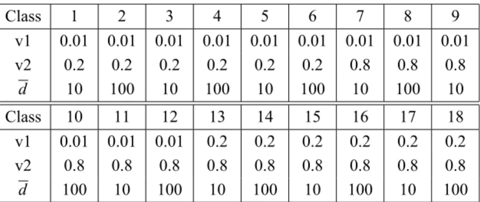
As in Foester and Wascher’s work [7], we generated 18 classes of random problems by combining different values of the generator’s parameters:
• v1assumed values 0.01 and 0.2; • v2assumed values 0.2 and 0.8;
• the number of items in the original cutting plan, denoted bymwas set to 10 (small instances), 20 (mid-size instances) and 40 (large instances);
• problems with low average demand (d = 10) and high average demand (d =100);
• In all the classesW =1000.
Each class contains 100 instances. We generated six classes with small items (v1 =0.01 andv2 =0.2), six classes with wide-spread items (v1 = 0.01 and v2=0.8) and other six classes with large items (v1=0.2 andv2=0.8). Table 1 shows the 18 classes and theirs parameters.
The solutions obtained by NANLCP were compared with the solutions of the methods: SHP [11], KOMBI234 [7] and ANLCP [17]. These methods (not including ANLCP) were also used as basis of comparison by Umetami et al. [19] with the heuristic APG. We run CUTGEN1 with the same seed (i.e.,1994) and parameters defined in [7] and [19] to generate all the 1800 instances (i.e., 18 classes, each class with 100 instances).
Class 1 2 3 4 5 6 7 8 9 v1 0.01 0.01 0.01 0.01 0.01 0.01 0.01 0.01 0.01
v2 0.2 0.2 0.2 0.2 0.2 0.2 0.8 0.8 0.8
d 10 100 10 100 10 100 10 100 10
Class 10 11 12 13 14 15 16 17 18
v1 0.01 0.01 0.01 0.2 0.2 0.2 0.2 0.2 0.2
v2 0.8 0.8 0.8 0.8 0.8 0.8 0.8 0.8 0.8
d 100 10 100 10 100 10 100 10 100
Table 1 – Random generated classes and their parameters.
The methods NANLCP and ANLCP and the heuristic SHP were implemented by the authors in Fortran, running under g77 for Linux, in a Athlon XP 1800Mhz, 512MB of RAM. The results for KOMBI234 were obtained from an implementa-tion in MODULA-2 in MSDOS operating system with a IBM 486/66. Therefore, the time was not considered when the comparison is done with KOMBI234.
Below, we present the computational results. We fixc1, the cost for each object used, equal to 1 andc2, the setup cost, equal to 100. The value ofc2can be seen as a penalization parameter for the setup number.
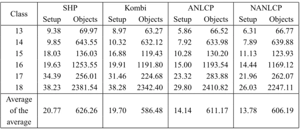
Tables 2, 3 and 4 show the average of the setup number and the average of the number of objects used in the final solution of the 100 instances in all the classes: small items, wide-spread items and large items. The averages of setup and number of objects described in the end of each table suggest that the NANLCP has a better performance than ANLCP, Kombi234 and SHP.
Table 5 presents the variation of setup and number of objects of the method (NANLCP) in relation to SHP. For instance, to compute the variation for the setup number we use the formula
100×(SetupNANLCP−SetupSHP)/SetupSHP,
SHP Kombi ANLCP NANLCP Class
Setup Objects Setup Objects Setup Objects Setup Objects
1 3.95 14.17 3.40 11.49 3.14 18.44 3.01 14.84
2 5.94 116.47 7.81 110.25 4.66 116.66 4.76 119.62
3 5.00 25.29 5.89 22.13 4.88 25.18 4.91 24.26
4 7.31 225.33 14.26 215.93 7.16 226.72 7.16 223.91
5 6.87 46.89 10.75 42.96 7.02 45.64 7.04 45.96
6 10.81 433.59 25.44 424.71 10.96 432.68 10.84 433.29 Average
of the 6.65 143.62 11.26 137.91 6.30 144.22 6.29 143.64 averages
Table 2 – Averages for small items.
SHP Kombi ANLCP NANLCP
Class
Setup Objects Setup Objects Setup Objects Setup Objects
7 8.84 55.84 7.90 50.21 5.78 50.84 5.31 53.69
8 9.76 515.76 9.96 499.52 8.22 506.02 6.97 488.85 9 17.19 108.54 15.03 93.67 10.90 106.72 10.92 105.65 10 19.37 1001.59 19.28 932.32 14.56 969.40 12.80 932.67 11 32.20 202.80 28.74 176.97 19.80 220.46 21.12 216.67 12 37.25 1873.05 37.31 1766.20 25.58 1813.60 25.25 1839.63 Average
of the 20.77 626.26 19.70 586.48 14.14 611.17 13.78 606.19 average
Table 3 – Averages for wide-spread items.
SHP Kombi ANLCP NANLCP
Class
Setup Objects Setup Objects Setup Objects Setup Objects
13 9.38 69.97 8.97 63.27 5.86 66.52 6.31 66.77
14 9.85 643.55 10.32 632.12 7.92 633.98 7.89 639.88 15 18.03 136.03 16.88 119.43 10.28 130.20 11.13 123.93 16 19.63 1253.55 19.91 1191.80 15.00 1193.54 14.44 1169.12 17 34.39 256.01 31.46 224.68 23.32 283.88 21.96 262.07 18 38.23 2381.54 38.28 2342.40 29.80 2410.82 26.03 2247.11 Average
of the 20.77 626.26 19.70 586.48 14.14 611.17 13.78 606.19 average
NANLCP versus SHP – Variation cost in relation to
Class Setup Object Class Setup Object Class Setup Object
Number Number Number Number Number Number
1 –23.80 +4.73 7 –39.93 –3.85 13 –32.73 –4.57
2 –19.87 +2.70 8 –28.59 –5.22 14 –19.90 –0.57
3 –1.80 –4.07 9 –36.47 –2.66 15 –38.27 –8.90
4 –2.05 –0.63 10 –33.92 –6.88 16 –26.44 –6.74
5 +2.47 –1.98 11 –34.41 +6.84 17 –36.14 +2.37
6 +0.28 –0.07 12 –32.21 –1.78 18 –31.91 –5.64
Table 5 – Variation in % of NANLCP in relation to SHP.
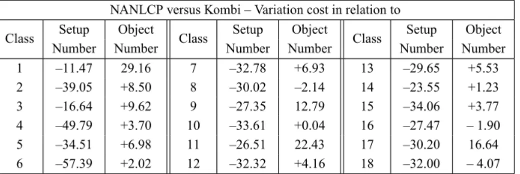
NANLCP versus Kombi – Variation cost in relation to
Class Setup Object Class Setup Object Class Setup Object
Number Number Number Number Number Number
1 –11.47 29.16 7 –32.78 +6.93 13 –29.65 +5.53
2 –39.05 +8.50 8 –30.02 –2.14 14 –23.55 +1.23
3 –16.64 +9.62 9 –27.35 12.79 15 –34.06 +3.77
4 –49.79 +3.70 10 –33.61 +0.04 16 –27.47 – 1.90
5 –34.51 +6.98 11 –26.51 22.43 17 –30.20 16.64
6 –57.39 +2.02 12 –32.32 +4.16 18 –32.00 – 4.07
Table 6 – Variation in % of NANLCP in relation to Kombi.
Table 6 presents the variation of setup and the number of objects of our method (NANLCP) in relation to KOMBI234. In all the classes NANLCP obtained a better average for the setup than KOMBI. But, the average number of objects used by KOMBI was better than NANLCP in the 15 classes.
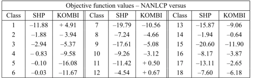
When comparing the quality of the solutions of each method, we usec2equal 5 and 10 in the objective function. Those are “real life” values for c2 and by doing so, the comparison with the others methods were more honest. In general, NANLCP obtained better objective function values than SHP and KOMBI.
The results obtained by NANLCP when c1 = 1 e c2 = 5 are presented in Table 7. The averages for the objectives function values for NANLCP were better than those obtained by SHP in all 18 classes an better than KOMBI in 15 classes.
The computational results confirm the good performance of NANLCP method. The version NANLCP, as shown in Table 8, obtained average costs better than SHP in 16 classes and better than KOMBI in all the classes.
Objective function values – NANLCP versus
Class SHP KOMBI Class SHP KOMBI Class SHP KOMBI
1 –11.88 + 4.91 7 –19.79 –10.56 13 –15.87 –9.06
2 –1.88 – 3.94 8 –7.24 –4.66 14 –1.94 –0.64
3 –2.94 –5.37 9 –17.61 –5.08 15 –20.60 –11.90
4 – 0.83 –9.58 10 –9.26 –3.12 16 –8.17 –3.87
5 –0.10 –16.08 11 –11.42 + 0.50 17 –13.11 –2.65
6 –0.03 –11.67 12 –4.54 + 0.67 18 –7.60 –6.18
Table 7 – Variation in % of the objective function value, withc1 = 1 e c2 = 5, of NANLCP in relation to SHP and KOMBI.
Objective Function Values – NANLCP versus
Class SHP KOMBI Class SHP KOMBI Class SHP KOMBI
1 –16.27 –1.21 7 –25.96 –17.35 13 –20.70 –15.10
2 –4.92 –11.22 8 –8.94 –6.77 14 –3.14 –2.25
3 –2.56 –9.47 9 –23.39 –11.94 15 –25.64 –18.39
4 –0.98 –17.58 10 –11.26 –5.73 16 –9.40 –5.56
5 +0.67 –22.66 11 –18.47 –7.86 17 –19.71 –10.68
6 +0.00 –20.24 12 –6.83 –2.20 18 –9.28 –7.99
Table 8 – Variation in % of the objective function value, withc1 = 1 ec2 = 10, of NANLCP in relation to SHP and KOMBI.
6 Conclusions and future work
object number and setup. Specifically in relation to Setup Number, NANLCP has a better performance than SHP and KOMBI in almost all the classes.
It is important to say that another advantage of NANLCP is the possibility of working with explicit values ofc1andc2 in the objective function. In fact, for real life problems these costs depend on many factors as demand, deadline, labor costs, etc. We do not know any other method that treat the problem of minimizing the setup and the number of processed object in the same way NANLCP does.
Computational time (in seconds)
Class SHP KOMBI ANLCP NANLCP
1 0.01 0.14 0.80 0.83
2 0.08 1.14 1.17 1.21
3 0.17 1.74 0.47 0.94
4 0.21 16.00 0.94 1.22
5 0.27 38.03 0.58 0.89
6 0.31 379.17 0.93 1.02
7 0.01 0.07 16.49 13.44
8 0.02 0.20 8.96 16.51
9 0.04 3.37 69.11 75.81
10 0.06 3.25 77.21 142.02
11 0.22 36.26 185.53 168.67
12 0.32 76.31 318.54 420.53
13 0.01 0.08 4.44 5.12
14 0.02 0.13 1.95 4.44
15 0.03 1.81 29.36 61.68
16 0.04 2.60 26.30 78.34
17 0.16 50.93 248.62 250.04
18 0.24 70.94 443.66 390.75
Table 9 – Average time (in seconds) for each method.
20 initial solutions to (hopefully) get rid of local minimum. For classes with a large numbers of items, as Classes (11, 12, 17, 18) the computational time for NANLCP was high.
Implementing better strategies to obtain global solutions when solving non-linear problems, can make NANLCP better. Also, a better strategy to obtain a integer solution from a fractional solution is welcome since the BRURED method used here is very naive, although, it is fast.
Acknowledgements. The authors appreciate the constructive comments of the referee, resulting in an improved presentation.
REFERENCES
[1] J.M. Allwood and C.N. Goulimins,Reducing the number of patterns in one-dimensional cutting stock problems. Control Section Report EE/CON/IC/88/10, Industrial Systems Group, Department of Electrical Engineering, Imperial College, London, (1988).
[2] G. Belov and G. Scheithauer,The number of setups (different patterns) in one-dimensional stock cutting. Technical Report, Dresden University (2003).
[3] A. Diegel, M. Chetty, S. Van Schalkwyck and S. Naidoo,Setup combining in the trim loss problem – 3-to-2 & 2-to-1. Working paper, Business Administration, University of Natal, Durban, First Draft (1993).
[4] A. Diegel, E. Montocchio, E. Walters, S. Schalkwyk and S. Naidoo,Setup minimising condi-tions in the trim loss problem. European J. Oper. Res.,95(1996), 631–640.
[5] H. Dyckhoff,A typology of cutting and packing problems. European J. Oper. Res.,44(1990), 145–159.
[6] H. Dyckhoff and U. Finke,Cutting and Packing in Production and Distribution: A Typology and Bibliography. Springer-Verlag, Berlin Heidelberg, 1992.
[7] H. Foester and G. Wascher,Pattern Reduction in One-dimensional Cutting-Stock Problems. International Journal of Prod. Res.,38(2000), 1657–1676.
[8] T. Gau and G. Wascher,CUTGEN1: A Problem Generator for the Standard One-dimensional Cutting Stock Problem. European J. Oper. Res.,84(1995), 572–579.
[9] P.C. Gilmore and R.E. Gomory,A Linear Programming Approach to the Cutting Stock Problem. Oper. Res.,9(1961), 849–859.
[10] P.C. Gilmore and R.E. Gomory, A Linear Programming Approach to the Cutting Stock Problem. Oper. Res.,11(1963), 863–888.
[12] R. Haessler,A Note on Computational Modifications to the Gilmore-Gomory Cutting Stock Algorithm. Oper. Res.,28(1980), 1001–1005.
[13] C.J. Hardley,Optimal cutting of zinc-coated steel strip. Oper. Res.,4(1976), 92–100.
[14] N. Krejic and J.M. Martinez,Validation of an Augmented Lagrangian algorithm with a Gauss-Newton Hessian approximation using a set of hard-spheres problems. Comput. Optim. Appl.,
16(2000), 247–263.
[15] R.E. Johnston,Rounding algorithms for cutting stock problems. Asia-Pacic. J. Oper. Res.,
3(1986), 166–171.
[16] J.M. Martinez,Minimization of discontinuous cost functions by smoothing. Acta Applicandae Mathematical,71(2001), 245–260.
[17] A.C. Moretti and L.L. Salles Neto,Modelo não-linear para minimizar o número de objetos processados e o setup num problema de corte unidimensional. Anais do XXXVII Simpósio Brasileiro de Pesquisa Operacional, Gramado, (2005) 1677–1688.
[18] H. Stadler, A one-dimensional cutting stock problem in the aluminium industry and its solution. European J. Oper. Res.,44(1990), 209–223.
[19] S. Umetami, M. Yagiura and T. Ibaraki,One Dimensional Cutting Stock Problem to Minimize the Number of Different Patterns. European J. of Oper. Res.,146(2003), 388–402.
[20] F. Vanderbeck,On Dantizg-Wolfe decomposition in integer programming and ways to per-form branching in a branch-and-price algorithm. Research Papers in Management Studies, University of Cambridge, 1994–1995, no. 29.
[21] F. Vanderbeck,Computational Study of a Column Generation Algorithm for Bin Packing and Cutting Stock Problems. Mathematical Programming,86(3) (1999), pp. 565–594.
[22] F. Vanderbeck,Exact Algorithm for Minimizing the Number of Setups in the one-dimensional cutting stock problem. Operations Research,48(2000), pp. 915–926.