The use of piezoelectric stress stiffening to enhance buckling
of laminated plates
Abstract
A technique for enhancement of buckling loads of composite plates is proposed. The technique relies on using stress stiff-ening to create a non-zero tensile force acting along the plate plane which ultimately permits the application of higher ex-ternal compressive forces that lead to traditional buckling instabilities. The idea is to completely restrain the plate movements in its plane direction, at all edges, and to ap-ply voltages to pairs of symmetrically bonded piezoelectric patches. This voltage is applied such that the piezoelectric patches contract resulting in a uniform tensile force over the plate plane.
Keywords
buckling, piezoelectric, stress stiffening, composites
Alfredo R. de Fariaa,∗ and
Maur´ıcio V. Donadonb
aInstituto Tecnol´ogico de Aeron´autica, CTA
- ITA - IEM, S˜ao Jos´e dos Campos, SP
12228-900, Tel.: 39475901; fax: 55-12-39475967 – Brazil
bInstituto Tecnol´ogico de Aeron´autica, CTA
- ITA - IEA, S˜ao Jos´e dos Campos, SP
12228-900, Tel.: 39475944; fax: 55-12-39475824 – Brazil
Received 27 Nov 2009; In revised form 24 Mar 2010
∗Author email: [email protected]
1 INTRODUCTION
Buckling of laminated plates caused by several types of loadings (mechanical, thermal, etc.) is one of the most relevant problems encountered in the area of composite structures. One technique available to increase buckling loads of this type of structure is to incorporate active elements, sensors and actuators, and control systems to such structures. Hence, these systems composed of host composite structure, active elements and control may have their buckling load increased with respect to the buckling load of the host structure if isolatedly considered. A number of materials and devices are available to implement active control. However, piezoelectric materials are again gaining popularity since their boom in the eighties [4] and nineties [10, 14]. Several investigations using the electromechanical properties of these mate-rials are concerned with active control of vibrations, noise suppression, flutter control, shape control and buckling load optimization.
Chandrashenkhara and Bathia [3] presented a finite element formulation to study the stabil-ity of laminated plates with integrated piezoelectric sensors and actuators. The finite element model is based on the theory of Reissner-Mindlin.
They concluded that the buckling load of this beam could be greater than the buckling load of the same beam without the action of the elements piezoelectric. Refined plate theories that account for piezoeletric effects are available in Refs. [2, 8]. A survey of such theories can be found in Ref. [7]. These refined theories address specially the kinematic relations in the displacement and electric fields. However, for the present work, a thin composite plate suited for aerospace applications is modeled and investigated. Hence, the theoretical formulation of laminated plates with layers of piezoelectric actuators and sensors using the Reissner-Mindlin plate theory contained in Ref. [12] shall be adopted.
Donadon et al. [6] investigated the efficiency of the use of piezoelectric elements in the
enhancement of natural frequencies of laminated plates. A finite element formulation was pro-posed for the analysis of laminated plates with an arbitrary number of piezoelectric actuators
and sensors. Nonlinear strain×displacement von Karman relations were used and a linear
be-havior was assumed for the electric degrees of freedom. Different configurations were analyzed both numerically and experimentally. The piezoelectric stress stiffening effect, also considered in the present work, is used to increase natural frequencies of composite plates.
de Faria [5] proposed the use of piezoelectric stiffening stresses to create a nonzero traction force acting along the axis of a laminated beam, allowing the application of an external com-pressive force greater than the buckling load of this beam without the presence of piezoelectric actuators. It was shown that the actuators’ length interfere with the intensity of the traction force piezoelectrically induced. However, the position of these actuators along the length of the beam does not alter the intensity of the traction force.
Kundun et al. [9] used the theory of nonlinear large deformations to study post-buckling of
piezoelectric laminated shells with double curvature through the finite element method. Batra and Geng [1] and Shariyat [13] present proposals to enhance dynamic buckling of flexible plates.
2 PROBLEM FORMULATION
The equations that describe the electromechanical behavior of a plate containing layers of the piezoelectric actuators bonded on its top and bottom surfaces are presented. The buckling analysis of the laminated plate is based on the Mindlin plate theory and the electric potential is assumed constant over the surface of the piezoelectric layers and varying linearly along the thickness of these layers.
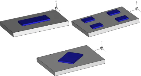
The basic configuration of the host structure consists of a rectangular plate equipped with patches of piezoelectric actuators symmetrically bonded to the top and bottom surfaces. Figure 1 shows three situations where there are pairs of piezoelectric actuators bonded to the bottom and top plate surface. In the prebuckling phase, only in-plane displacements and stresses arise. When nonzero voltages are equally applied to the top and bottom piezoelectric
patches displacementsuandv result. In this phase the boundary conditions assumed are that
of completely constrained edges with u = v = 0. If the plate’s edges were free to move then
there would be no piezoelectric stiffening stresses. Once the piezoelectric patches are energized traditional mechanical forces uniformly distributed along the edges and usually denoted by
Nxx0, Nyy0, Nxy0 are slowly applied causing compressive and shear stresses that eventually buckle the plate. In a testing facility forces Nxx0,Nyy0,Nxy0 would possibly be the result of prescribed displacements.
Figure 1 Basic configurations
The constitutive equations can be written as in Eq. (1) where it is assumed that the piezoelectric layers are polarized along thez direction (perpendicular to the plate).
σ=Qϵ−eTE, τ =QSγ, d=eϵ+ξE, (1)
are the out-of-plane shear srains,d is the electric displacement,E is the electric field,eis the electro-mechanical coupling matrix andξ is the permitivitty matrix. Notice that τ is free of piezoelectric effects [8]. Equation (1) is valid in general for both composite and piezoelectric
material. In the case of a composite layer matriceseand ξ would vanish.
The system is conservative such that the total potential energy is given by:
Π= 1
2∫V σ TϵdV
+1
2∫V τ TγdV
−1
2∫Vd TEdV
−W, (2)
where W is the work of external forcesNxx0,Nyy0,Nxy0.
The Mindlin plate displacement field is now introduced:
˜
u(x, y, z) = u(x, y)+zψx(x, y),
˜
v(x, y, z) = v(x, y)+zψy(x, y),
˜
w(x, y, z) = w(x, y), (3)
where ˜u, ˜v, ˜w are the displacements of an arbitrary point in the plate, u, v, w are the mid plane displacements (z =0) and ψx, ψy are the mid plane rotations. The strains ϵ can now
be split into three components: membrane strains ϵ0, curvatureκ and nonlinear von Karman
strainsϵN such that
ϵ=ϵ0+zκ+ϵN =⎧⎪⎪⎪
⎨⎪⎪⎪ ⎩
u,x
v,y
u,y+v,x
⎫⎪⎪⎪ ⎬⎪⎪⎪ ⎭
+z⎧⎪⎪⎪⎨⎪⎪⎪ ⎩
ψx,x
ψy,y
ψx,y+ψy,x
⎫⎪⎪⎪ ⎬⎪⎪⎪ ⎭
+1
2
⎧⎪⎪⎪ ⎨⎪⎪⎪ ⎩
w2,x w,y2
2w,xw,y
⎫⎪⎪⎪ ⎬⎪⎪⎪ ⎭ ,
γ={ w,x+ψx w,y+ψy }
. (4)
In order to facilitate manipulation of Eq. (2) matrices A, B, D and AS, and
vec-tors N= { Nxx Nyy Nxy }T, M = { Mxx Myy Mxy }T, Q = { Qxx Qyy }T and F =
{ Fxx Fyy Fxy }T are defined as
(A,B,D) = ∫
h/2
−h/2(
1, z, z2)Qdz
AS = ∫
h/2
−h/2
QSdz
F = ∫
h/2
−h/2
eTEdz
{ MN } = [ A B
B D ]{
ϵ0+ϵN
κ }
where h is the total thickness. Following conventional terminology, the components of N are
the in-plane forces per unit length, the components of Q are the out-of-plane shear forces
per unit length, the components of F are the piezoelectric in-plane forces per unit length
and the components of M are bending moments per unit length. From this point on these
will be simply referred to as forces or moments. Notice that the piezoelectric layers make a contribution to the laminate stiffness matricesA,B,Dand AS. On the other hand, vectorF
is nonzero only if there are piezoelectric layers present in the laminate. F can be interpreted as the piezoelectric force. If the electric field Ez is replaced byφ/twhereφ is voltage andt is
thickness then Eq. (5c) can be specialized to become [11]
⎧⎪⎪⎪ ⎨⎪⎪⎪ ⎩
Fxx
Fyy
Fxy
⎫⎪⎪⎪ ⎬⎪⎪⎪ ⎭
=⎧⎪⎪⎪ ⎨⎪⎪⎪ ⎩
e31(φT +φB)
e32(φT +φB) 0
⎫⎪⎪⎪ ⎬⎪⎪⎪ ⎭
, (6)
where φT and φB are the voltages applied to the top and bottom surfaces of the plate. In
practical applicationse32=e31 what leads toFxx=Fyy.
Taking the first variation of Eq. (2), assuming that the voltages are prescribed and inte-grating through the thickness yields
δΠ=∫
Ω(
NTδϵ0+NTδϵN+MTδκ+QTδγ−FTδϵ0−FTδϵN)dΩ−
∫Γ(Nxx
0, Nxy0)⋅n δud⃗ Γ−∫ Γ(Nxy
0, Nyy0)⋅n δvd⃗ Γ=0, (7) where Ω is the in-plane plate domain, Nxx0, Nyy0, Nxy0 are membrane forces applied along the plate edge Γ (the boundary of Ω),⃗nis the unit vector normal to Γ and the term containing
zFTδκ was abandoned since full symmetry (φT = φB) has been admitted. Notice that if
φT ≠ φB then the prebuckling problem would result in nonzero out-of-plane displacements
(w≠0) and no bifurcation type buckling would occur.
Substitution of Eqs. (4) into Eq. (7) and integration by parts in two dimensions allows one to obtain the governing equations
(Nxx−Fxx),x+(Nxy−Fxy),y=0
(Nxy−Fxy),x+(Nyy−Fyy),y=0
Mxx,x+Mxy,y=Qxx
Myy,y+Mxy,x=Qyy
Qxx,x+Qyy,y+(Nxx−Fxx)w,xx+(Nyy−Fyy)w,yy+2(Nxy−Fxy)w,xy=0 (8)
and in-plane boundary conditions valid on the plate’s edges:
(Nxx−Fxx, Nxy−Fxy)⋅n δu⃗ = (Nxx0, Nxy0)⋅n δu⃗
Notice that there are three more boundary conditions related to δw,δψx,δψy that, although
indispensable to solve the buckling eigenproblem, are not given in Eq. (9).
Terms (Nxx−Fxx),(Nxy−Fxy) and (Nyy−Fyy) present in Eqs. (8) and (9) correspond
to the piezoelectric stiffening stress resultants. Hence, if there are no piezoelectric stiffening stresses then buckling cannot occur due to the piezoelectric effect. There are two possibilities for buckling to occur: (i) external mechanical forcesNxx0,Nyy0orNxy0must be present (this is the traditional buckling problem) and (ii) nonzero piezoelectric stiffening stresses must exist. Situation (ii) is the subject of next section.
3 PIEZOELECTRIC STIFFENING STRESSES
In order to obtain the piezoelectric stiffening stress distribution it is necessary to solve the prebuckling Eqs. (8a) and (8b) along with their boundary conditions in Eq. (9). Unfortunately, this problem does not admit an exact analytical solution mainly because of the discontinuity caused by the presence of piezoelectric patches bonded to the plate surfaces. The patches are source of two kinds of discontinuity: stiffness and piezoelectric force. It is clear that adding piezoelectric layers to the laminate increases the in-plane stiffness matrixA. It is also clear that the piezoelectric forcesFxx,Fyy,Fxyare nonzero only when piezoelectric patches are attached,
that is, over the regions of the plate where there are no actuatorsFxx=Fyy=Fxy=0.
The bifurcation type buckling is the subject of this paper. The objective is to enhance the critical buckling load of plates that exhibit such type of buckling by appropriately tailoring the piezoelectric stiffening stresses. Therefore, this study is concerned with cases where there are
no out-of-plane displacements w in the prebuckling regime. This can only be achieved when
there is full symmetry on the actuators part (φT =φB) and when the laminate is symmetric
(B = 0 and tT = tB). If these conditions apply and the nonlinear strain components are
neglected in the prebuckling regime then Eq. (7) can be simplified to:
δΠ=∫
Ω
⎧⎪⎪⎪ ⎨⎪⎪⎪ ⎩
δu,x
δv,y
δu,y+δv,x
⎫⎪⎪⎪ ⎬⎪⎪⎪ ⎭
T
⎛ ⎜ ⎝ ⎡⎢ ⎢⎢ ⎢⎢ ⎣
A11 A12 A16
A12 A22 A26
A16 A26 A66
⎤⎥ ⎥⎥ ⎥⎥ ⎦
⎧⎪⎪⎪ ⎨⎪⎪⎪ ⎩
u,x
v,y
u,y+v,x
⎫⎪⎪⎪ ⎬⎪⎪⎪ ⎭
−⎧⎪⎪⎪⎨⎪⎪⎪ ⎩
Fxx
Fyy
Fxy
⎫⎪⎪⎪ ⎬⎪⎪⎪ ⎭ ⎞ ⎟
⎠dΩ=0. (10)
Analytical solution of Eq. (10) is not possible. However, it is possible to gain insight into the problem if a symmetric configuration is investigated. Assume that only one rectangular piezoelectric patch is placed in the center of the plate such as depicted in Fig. 2. Taking
u(x, y) as the displacements along x and v(x, y) as the displacements along y the symmetry and boundary conditions are:
• Edgey=0: v(x,0)=v,x(x,0)=v,xx(x,0)=...=0,u,y(x,0)=0;
• Edgex=0: u(0, y)=u,y(0, y)=u,yy(0, y)=...=0,v,x(0, y)=0;
• Edgey=Ly: v(x, Ly)=v,x(x, Ly)=v,xx(x, Ly)=...=0,u,y(x, Ly)=0;
Lx
Ly
lx
ly plate + piezo
plate
x y
A B
Figure 2 Basic dimensions
Conditions v(x,0)=0,u(0, y)=0, u,y(x,0)=0, v,x(0, y)=0 follow from the symmetry of
the problem. v(x, Ly) =0 and u(Lx, y) =0 are enforced boundary conditions. u,y(x, Ly) =0
andv,x(Lx, y)=0 result from the requirements thatNxy(x, Ly)=Nxy(Lx, y)=0 for a balanced
laminate (A16=A26=0) as given in Eq. (9). The boundary condition in Eq. (9) also imposes that continuity on Nxx−Fxx and Nxy−Fxy along any line of constant y must be satisfied
as well as continuity on Nxy−Fxy and Nyy−Fyy along any line of constant x. Moreover,
continuity of displacementsu and v throughout must be observed.
Considering the lines y =0, x =0 and a balanced laminate, the continuity conditions on
Nxx−Fxx for pointA and Nyy−Fyy for pointB read, respectively,
A∗
11u∗,x(lx,0)+A∗12v,y∗(lx,0)−Fxx = A11u,x(lx,0)+A12v,y(lx,0),
A∗
12u∗,x(0, ly)+A∗22v,y∗(0, ly)−Fyy = A12u,x(0, ly)+A22v,y(0, ly). (11)
where the terms with a superscript star (∗) refer to domain where there are both plate and
piezoelectric materials. From Eqs. (11) it can be seen that there must be discontinuity on
u,x(x,0) and v,y(0, y). A finite element that enforces continuity on the first derivatives of u
and v, such as the one based on the classical plate theory, would not be a good choice in this case. A better suited element for this task is the one based on Mindlin assumptions that are able to capture discontinuities on the first derivatives of u and v, whose description is in the next section.
Since exact solutions to Eq. (10) cannot be obtained it remains to find analytical approx-imations or numerical solutions. One approach to obtain approxapprox-imations is to consider that the plate shown in Fig. 2 behaves similarly to a beam, at least along the lines y= 0, x =0.
problems. Therefore, the governing differential equations can be simplified to u,xx(x,0) = 0
and v,yy(0, y)=0. Moreover, Eqs. (11) reduce to
A∗
11u∗,x(lx,0)−Fxx = A11u,x(lx,0),
A∗
22v,y∗(0, ly)−Fyy = A22v,y(0, ly). (12)
Considering the boundary conditions u(0,0)=u(Lx,0)=0 and v(0,0)=v(0, Ly)=0, and
the jump conditions in Eq. (12), the differential equationsu,xx(x,0)=0 and v,yy(0, y)=0 are
solved to yield:
u∗(x,0)= (
1
Lx − 1
lx)xFxx
[A∗
11( 1
Lx − 1
lx)−A11 1
Lx]
, u(x,0)= (
x
Lx−1)Fxx
[A∗
11( 1
Lx− 1
lx)−A11 1
Lx]
,
v∗(0, y)= (
1
Ly − 1
ly)yFyy
[A∗
22( 1
Ly − 1
ly)−A22 1
Ly]
, v(0, y)= (
y
B−1)Fyy
[A∗
22( 1
Ly − 1
ly)−A22 1
Ly]
. (13)
The piezoelectric stiffening stress resultants are given by:
Txx=A∗11u∗,x(x,0)−Fxx=A11u,x(x,0)=
Fxx A∗
11
A11(1−
Lx
lx)−1
,
Tyy=A∗22v,y∗(0, y)−Fyy=A22v,y(0, y)=
Fyy A∗
22
A22(1−
Ly
ly )−1
. (14)
A numerical example requires physical properties given in Tab. 1 and geometric
param-eters. The plate is assumed to have semi-length Lx = 0.2 m, semi-width Ly = 0.15 m. The
piezoelectric actuator has semi-length lx = 0.15 m and semi-width ly = 0.05 m. A cross-ply
laminate [0/90]S is used with each layer 0.15 mm thick. The thickness of the piezoelectric
actuators (top and bottom) is 0.05 mm. A voltage of φT = φB = 50 V is applied which
corresponds exactly to the depoling field in Tab. 1.
Figures 3 and 4 present a comparison between the analytical solutions given in Eq. (13) and the FE numerical solution, where ξ =x/Lx and η =y/Ly. It is clear that the analytical
solution along y = 0 is a very good approximation to the actual displacements. Both u and
u,x agree well. However, the same is not true for analytical solution along x = 0. It can be
observed that, although the patterns for v and v,y are similar in shape, their magnitudes are
completely dispair. The conclusion is that, in this particular configuration, the plate behaves much like a beam in the xdirection but not in the y direction.
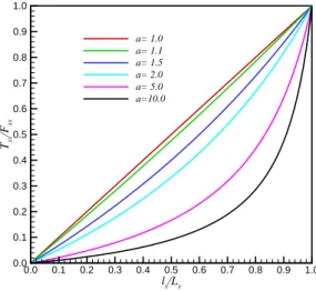
Closer observation of Eq. (14) reveals that the piezoelectric stiffening stress resultants depend basically on two parameters: the relative stiffnessa=A∗
Table 1 Physical properties
Property G1195N T300/5208
Young modulus E11 (GPa) 63.0 154.5
Young modulus E22 (GPa) 63.0 11.13
Poisson ratio ν12 0.3 0.304
Shear modulusG12=G13 (GPa) 24.2 6.98
Shear modulusG23 (GPa) 24.2 3.36
Piezoelectric constante31 (N/V m) 17.6
-Piezoelectric constante32 (N/V m) 17.6
-Depoling fieldEMAX (V/mm) 1000
-ξ
u,x
-1.0 -0.5 0.0 0.5 1.0
-3.0E-05 -2.0E-05 -1.0E-05 0.0E+00 1.0E-05
FEM analytic
ξ
u
/Lx
-1.0 -0.5 0.0 0.5 1.0
-8.0E-06 -6.0E-06 -4.0E-06 -2.0E-06 0.0E+00 2.0E-06 4.0E-06 6.0E-06 8.0E-06
FEM analytic
Figure 3 Comparison FEM vs. analytical solutions alongy=0
η
v/
Ly
-1.0 -0.5 0.0 0.5 1.0
-8.0E-05 -6.0E-05 -4.0E-05 -2.0E-05 0.0E+00 2.0E-05 4.0E-05 6.0E-05 8.0E-05
FEM analytic
η
v,y
-1.0 -0.5 0.0 0.5 1.0
-1.5E-04 -1.0E-04 -5.0E-05 0.0E+00 5.0E-05 1.0E-04 1.5E-04 2.0E-04 2.5E-04
FEM analytic
5 shows that, the smaller a, the greater is the efficiency to generate piezoelectric stiffening stresses. Fortunately, in aerospace applications, thin piezoelectric actuators are used leading to practical situations where 1.0<a≤1.2.
lx/Lx
Txx
/F
xx
0.0 0.1 0.2 0.3 0.4 0.5 0.6 0.7 0.8 0.9 1.0 0.0
0.1 0.2 0.3 0.4 0.5 0.6 0.7 0.8 0.9 1.0
a= 1.0 a= 1.1 a= 1.5 a= 2.0 a= 5.0 a=10.0
Figure 5 Stress stiffening efficiency varying with relative stiffness
The stiffening stress resultantsNxxandNyyare shown in Fig. 6 where the boundary of the
piezoelectric actuator is highlighted in black. Notice that Nxx is highly discontinuous along
x=0 and so is Nyy along y=0. The discontinuities observed numerically are consistent with
Eq. (12). Additionally, the region where there is compression in the x direction (Nxx < 0)
is mostly limited to the region underneath the actuators. However, the same cannot be said about Nyy. This suggests that long piezoelectric film strips with large aspect ratios are able
to orient stiffening stresses more efficiently than those with aspect ratios close to unity.
4 PIEZOELECTRIC STRESS STIFFENING AND BUCKLING
Considering that the membrane prebuckling problem given in Eq. (10) is satisfied, the FEM buckling equations can be derived from Eq. (7) to yield
δΠ=∫
Ω(M
Tδκ
+QTδγ)dΩ+∫
Ω(N−F)
Tδϵ
NdΩ. (15)
The finite element method is used to solve the governing buckling problem Eq. (15). The element used is biquadratic depicted in Fig. 7 whose interpolation functions are:
N1(ξ, η)= 1
4ξ(ξ−1)η(η−1) N2(ξ, η)= 1 2(1−ξ
2
)η(η−1) N3(ξ, η)= 1
4ξ(ξ+1)η(η−1)
N4(ξ, η)= 1
2ξ(ξ−1)(1−η 2
) N5(ξ, η)=(1−ξ2)(1−η2) N6(ξ, η)= 1
2ξ(ξ+1)(1−η 2
) N7(ξ, η)=
1
4ξ(ξ−1)η(η+1) N8(ξ, η)= 1 2(1−ξ
2
)η(η+1) N9(ξ, η)= 1
332.9 271.6 210.3 149.0 87.7 26.4 -34.9 -96.2 -157.5 -218.8 -280.1 -341.4 -402.7 -464.0 -525.3 -586.6 -647.9 -709.2 -770.5 -831.8 Nyy(N/m)
87.9 11.9 -64.2 -140.2 -216.3 -292.3 -368.3 -444.4 -520.4 -596.5 -672.5 -748.6 -824.6 -900.7 -976.7 -1052.8 -1128.8 -1204.9 -1280.9 -1357.0 Nxx(N/m)
Figure 6 Stiffening stress distribution in terms of resultant forces
+1
+1
−1
1
2
4
3
5
6
7
8
9
−1
η
ξ
Figure 7 Biquadratic element
The interpolation functions given in Eq. (16) are used to interpolate five degrees of freedom per node: u,v,w,ψx and ψy. Hence the element contains a total of 45 degrees of freedom per
element. When Eqs. (4), (5) and (16) are introduced into the first integral of Eq. (15) the finite element stiffness matrixKarises. The biquadratic element is less prone to shear locking than the traditional bilinear element. However, the reduced selective integration scheme is
used to compute matrix K. The second integral in Eq. (15) contains the membrane forces
N and corresponds to a stiffening term (observe that it involves the nonlinear strains δϵN).
There are two types of contributions to N: (i) the traditional mechanical stresses N0 due to
Nxx0, Nyy0, Nxy0, and (ii) piezoelectric stiffening stresses Np computed through solution of
Eq. (10), such thatN=N0+Np. Therefore, two geometric stiffness matrices arise: KPG from
∫(Np−F)TδϵNdΩ andKG from ∫ NT0δϵNdΩ. Therefore, the complete FE buckling equation
(K+
p
∑
i=1
φiKPGi−λKG)q=0, (17)
whereK is the stiffness matrix,KPGiis the piezoelectric geometric stiffness matrix that incor-porates the piezoelectric stiffening stresses and is associated with piezoelectric pair i, KG is
the geometric stiffness matrix,λis the buckling load and qis the buckling mode. Notice that the formulation presented in Eq. (17) assumes that voltages of φi = 1 V are applied in order
to form matrixKPGi.
In order to obtain numerical results for buckling in the presence of piezoelectric stiffening stresses consider the plate used in the previous section (Lx = 0.2 m and Ly= 0.15 m) and one
rectangular actuator withlx= 4 cm andly= 3 cm placed in the center of the plate whose sides
are parallel to the sides of the plate. Two types of traditional loadings are applied: (i) uniform compressive loading along thexdirection (λxx) and uniform shear (λxy). The actuator voltage
is varied within the limits of the depoling field, i.e., -50 V ≤φ≤+50 V. Figure 8 presents the
curves obtained for the [0/90]S and [±45]S laminates. Points on those curves are obtained
through solution of Eq. (17) for different values of φ. Buckling occurs under no mechanical
loading (eitherNxx0=0 orNxy0=0) for some value ofφ>+50 V for both types of loading. This conclusion agrees with the expectation that, when positive voltages are applied, compressive stiffening stresses, as those illustrated in Fig. 6, arise, impairing buckling behavior. The first buckling modes for the [0/90]S laminate subject to λxx are presented in Fig. 9 for different
values of voltage. The differences between the mode shapes are not significant but the buckling load dramatically changes as seen in Fig. 8. However, the peaks of the normalized buckling modes, given in terms of transverse displacementsw, become increasingly higher as the voltage
is varied from -50 V to +50 V. The maximumλxx= 660 N/m andλxy= 870 N/m are associated
with φ= -50 V. It can be observed that the [±45]S laminate is less sensitive to variations in
φ. This is evidence that sensitivity to φ is associated with the laminate lay-up. The [±45]S
laminate will suffer from buckling due to stiffening stresses only for value of φ substantially above +50 V.
A better understanding of Fig. 8 is gained if a perturbation analysis of the buckling eigenproblem is performed. Assume that the voltage of pairiis slightly perturbed byδφisuch
that the new eigenproblem derived from Eq. (17) becomes
[K+
p
∑
i=1
(φi+δφi)KPGi−(λ+δλ+δ
2
λ+...)KG](q+δq+δ2q+...)=0, (18)
The zero-, first- and second-order problems derived from Eq. (18) are respectively
(K+
p
∑
i=1
φiKPGi−λKG)q=0
(∑p
i=1
δφiKPGi−δλKG)q+(K+
p
∑
i=1
φ(V)
λ
(N
/m
)
-50 -40 -30 -20 -10 0 10 20 30 40 50 0 250 500 750 1000 1250 1500 1750 2000
λxx[0/90]S λxy[0/90]S
λxx[±45]S
λxy[±45]S
Figure 8 Buckling load vs. voltage: one patch parallel to plate’s edges
0.0251 0.0238 0.0225 0.0212 0.0199 0.0186 0.0174 0.0161 0.0148 0.0135 0.0122 0.0109 0.0096 0.0084 0.0071 0.0058 0.0045 0.0032 0.0019 0.0006
φ= -50 V w 0.0293
0.0278 0.0263 0.0248 0.0233 0.0218 0.0203 0.0188 0.0173 0.0158 0.0143 0.0128 0.0113 0.0098 0.0083 0.0068 0.0053 0.0038 0.0023 0.0008
φ= -25 V w
0.0503 0.0477 0.0452 0.0426 0.0400 0.0374 0.0348 0.0323 0.0297 0.0271 0.0245 0.0219 0.0194 0.0168 0.0142 0.0116 0.0090 0.0065 0.0039 0.0013
φ= +25 V w 0.1663
0.1578 0.1493 0.1407 0.1322 0.1237 0.1151 0.1066 0.0981 0.0896 0.0810 0.0725 0.0640 0.0554 0.0469 0.0384 0.0299 0.0213 0.0128 0.0043
φ= +50 V w
(∑p
i=1
δ2φiKPGi−δ
2
λKG)q+(
p
∑
i=1
δφiKPGi−δλKG)δq+(K+
p
∑
i=1
φiKPGi−λKG)δ
2
q=0. (19)
Multiplication of Eq. (19b) by qT and using Eq. (19a) yields
δλ=
p
∑
i=1
qTKPGiq
qTK
Gq
δφi. (20)
Equation (20) shows that the sign of ∂λ/∂φi is related to the the positive-definiteness of
KPGi,KG and the buckling mode q. In the case of uniform compressive forces matrix KG is
positive-definite. However, the same cannot be said about KPGi. In fact, Fig. 6 indicates that the termNxx−Fxx is positive in some regions over the plate and negative over others. Hence,
the sign of qTKPGiqdepends ultimately on q. Figure 8 just confirms this finding.
Multiplication of Eq. (19c) by qT and using Eqs. (19a) and Eqs. (19b) yields
δ2λ=−
δqT(K+∑pi=1φiK
P
Gi−λKG)δq
qTK
Gq
. (21)
Matrix(K+∑φiKPGi−λKG)is positive-definite provided buckling has not occurred.
There-fore, the sign of δ2λgiven in Eq. (21) is certainly negative if KG is positive-definite. Notice
that this may not be the case when shear loadings are applied but it is true for the case where
Nxx0 ≠0 and Nxy0= Nyy0= 0. Figure 8 confirms that the concavity of the λ vs. φ curve is negative.
A network of piezoelectric actuators may be used to try to induce more favorable piezoelec-tric stiffening stresses. Figure 1b shows a possibility where the only patch shown in Fig. 1a is split into four smaller patches such that the total area is maintained constant. This procedure guarantees that, provided the same voltage is applied, the electric energy required is also the same. Figure 10 presents theλvs. φcurves obtained assuming that equal voltages are applied to the four patches. Comparison to Fig. 8 leads one to conclude that the normal and shear buckling loads were decreased for both the [0/90]S and [±45]S laminates. Therefore, this
particular procedure did not bring any improvement to the buckling loads. However, this sim-ulation suggests that the piezoelectric actuators should be placed as far from the boundaries as possible in order to boost the potential benefits of the piezoelectric stiffening stresses.
Figure 1c presents another possibility for placement of the actuators, i.e., patches with arbitrary orientation. In Fig. 1c the same rectangular patch of Figure 1a is used but it
is oriented parallel to the plate diagonal. Figure 11 presents the λ vs. φ curves obtained.
Comparison against Figs. 8 and 10 demonstrates that this configuration is the best one for both laminates wheneverφ<0 V and it has good performance forφ>0 V except for extreme
φ(V)
λ
(N
/m
)
-50 -40 -30 -20 -10 0 10 20 30 40 50 0
250 500 750 1000 1250 1500 1750 2000
λxx[0/90]S λxy[0/90]S
λxx[±45]S
λxy[±45]S
Figure 10 Buckling load×voltage: four patches parallel to plate’s edges
φ(V)
λ
(N
/m
)
-50 -40 -30 -20 -10 0 10 20 30 40 50 0
250 500 750 1000 1250 1500 1750 2000
λxx[0/90]S λxy[0/90]S
λxx[±45]S
λxy[±45]S
Figure 11 Buckling load×voltage: one patch parallel to plate’s diagonal
5 CONCLUSIONS
jump but it consists in an impractical alternative from the experimental point of view. The analytical solution obtained for the prebuckling regime is reasonable in the direction along which the piezoelectric patch is longer but yields unreasonable results in the shorter direction. Therefore, numerical procedures must be employed in order to obtain the pre-cise distribution of piezoelectric stiffening stresses. Although not suitable for exact solution, Eq. (8e) contains a very important message: buckling cannot occur if there are no stiffening stresses Nxx−Fxx,Nyy−Fyy orNxy−Fxy. Therefore, it proves that free-free structures, even
when equipped with piezoelectric actuators, will not buckle. The condition for the loss of sta-bility is that either external mechanical loadings are applied or piezoelectric stiffening stresses arise as a result of boundary constraints.
Numerical simulations considered two symmetric laminates: [0/90]S and [±45]S. These
were selected because the former is a typical lay-up in aeronautical construction and the later is the optimal lay-up against buckling in the normal direction (λxx). All the results show that
buckling behavior is improved for negative voltages and is impaired for positive voltages. This is obviously a result of piezoelectric stiffening stresses over the composite plate. As a practical recommendation piezoelectric actuators should have their orientations carefully chosen, but the most important finding is that they should be placed as far as possible from the edges in order to maximize the beneficial effects of the piezoelectric stiffening stresses.
Acknowledgements This work was partially financed by the Brazilian agency CNPq (grants no. 300236/2009-3 and 303287/2009-8).
References
[1] R. C. Batra and T. S. Geng. Enhancement of the dynamic buckling load for a plate by using piezoceramic actuators.
Smart Materials and Structures, 10(5):925–933, 2001.
[2] E. Carrera M. Boscolo and A. Robaldo. Hierarchic multilayered plate elements for coupled multifield problems of
piezoelectric adaptive structures: formulation and numerical assessment. Archives of Computational Methods in
Engineering, 14(4):383–430, 2007.
[3] K. Chandrashenkhara and K. Bathia. Active buckling control of smart composite plates - finite element analysis.
Smart Materials and Structures, 2(1):31–39, 1993.
[4] E. F. Crawley and J. de Luis. Use of piezoelectric actuators as elements of intelligent structures. AIAA Journal,
25(10):1373–1385, 1987.
[5] A. R. de Faria. On buckling enhancement of laminated beams with piezoeletric actuators via stress stiffening.
Composite Structures, 65(2):187–192, 2004.
[6] M. V. Donadon, S. F. M. Almeida, and A. R. de Faria. Stiffening effects on the natural frequencies of laminated
plates with piezoelectric actuators. Composites Part B: Engineering, 35(5):335–342, 2002.
[7] S. V. Gopinathan, V. V. Varadan, and V. K. Varadan. A review and critique of theories for piezoelectric laminates.
Smart Materials and Structures, 9(1):24–48, 2000.
[8] M. K¨ogl and M. L. Bucalem. A family of piezoelectric mitc plate elements.Computers & Structures, 83(15-16):1277–
1297, 2005.
[9] C. K. Kundun, D. K. Maiti, and P. K. Sinha. Post buckling analysis of smart laminated doubly curved shells.
Composite Structures, 81(3):314–322, 2007.
[10] T. Meressi and B. Paden. Buckling control of a flexible beam using piezoelectric actuators. Journal of Guidance,
[11] N. Y. Nye. Physical Properties of Crystals: their representation by tensors and matrices. Oxford University Press, 1972.
[12] J. N. Reddy.Mechanics of Laminated Composite Plates: Theory and Analysis. CRC Press, Boca Raton, 1997.
[13] M. Shariyat. Dynamic buckling of imperfect laminated plates with piezoelectric sensors and actuators subjected to
thermo-electro-mechanical loadings, considering the temperature-dependency of the material properties. Composite
Structures, 88(2):228–239, 2009.
[14] S. P. Thompson and J. Loughlan. The active buckling control of some composite column strips using piezoelectric