Universidade de Lisboa
Faculdade de Ciências
Departamento de Biologia Animal
Study on the diversification of flat periwinkles (Littorina fabalis and L. obtusata): insights from genetics and geometric morphometrics
João Gonçalo Monteiro Carvalho
Dissertação
Mestrado em Biologia Evolutiva e do Desenvolvimento 2014
Universidade de Lisboa
Faculdade de Ciências
Departamento de Biologia Animal
Study on the diversification of flat periwinkles (Littorina fabalis and L. obtusata): insights from genetics and geometric morphometrics
João Gonçalo Monteiro Carvalho
Dissertação
Mestrado em Biologia Evolutiva e do Desenvolvimento Dissertação orientada pela Professora Dra. Manuela Coelho e
Dr. Juan Galindo Dasilva 2014
1 Acknowledgments
Bem, demorou mas finalmente se conclui este capítulo da minha vida. Ao longo destes meses foram várias as pessoas com quem partilhei este caminho mas parece-me adequado começar pelas pessoas que me acompanharam em Vigo. Suponho que seja melhor escrever esta parte no meu espanhol limitado, por isso aqui vai: Sin un orden en particular, me gustaría comenzar haciendo referencia a Celeste y Eva por ayudarme en los primeros días en Vigo, cuando no conocía a nadie y no podía hacer un gel! Muchísimas gracias también a las chicas del café (Raquel, Ana, Nieves, Sara) porque siempre estáis alegres y muy amables! Para MJ, gracias por la compañía en las mazmorras y también por la música. A todas las personas en el grupo (Ángel, Andrés, Antonio, Armando, Emilio y Paloma) gracias porque siempre estabais amables conmigo y por crearen un ambiente de trabajo divertido. Tengo que mencionar el grupo de Comeeeeer!!! Por la compañía y las conversaciones humorísticas e interesantes durante la comida y el café posterior, gracias Lara, Dani (Nos vemos en Lisboa) y Belén! Por último, un agradecimiento muy especial a Mónica por cada momento de diversión, por todas las conversaciones y por aguantar con mis tonterías.
Hablar de Vigo es imposible sin hablar de Juan Galindo (XB2, Universidad de Vigo). También sería imposible enumerar todas las razones que tengo para darte las gracias. Desde tu paciencia con la burocracia de las universidades hasta tu paciencia con mis errores, pasando por todo lo que me has enseñado durante este tiempo. Gracias por todo lo que he aprendido contigo y por tu amabilidad y apoyo constante! Martín es un tío con suerte :)
Voltando agora ao idioma de Camões e Fernando Pessoa, vou aproveitar que falei do Juan para falar sobre o meu outro orientador, o Rui Faria (CIBIO, Universidade do Porto). Quero agradecer-te por me integrares na equipa do fascinante projecto de investigação que lideras, financiado pela FCT e FEDER (“The paths of parallel evolution and their genetic crossroads“ - PTDC/BIA-EVF/113805/2009), e que permitiu que esta tese fosse uma realidade. Quero também agradecer-te por tudo o
2 que me ensinaste, tanto na parte de análise de dados como na parte da escrita. Esta tese não teria metade da qualidade que tem sem as tuas correcções e melhorias. Obrigado também por todo o teu apoio e por acreditares em mim e principalmente por tudo o que me ensinaste sobre especiação em particular e sobre ciência em geral. Neste ultimo ponto, uma das coisas mais importantes foi perceber que apesar de ser difícil gerir e coordenar um grupo, é possível fazer isso mesmo e ao mesmo tempo criar um ambiente positivo onde várias questões científicas podem ser abordadas e debatidas.
Não posso falar do Rui sem referir as pessoas que trabalham neste grupo fantástico. Graciela, muchas gracias por toda tu ayuda con los micros y muchas otras cosas. Eres una persona incansable y espero que nunca cambies pues eres genial! Obrigado também a Diana pela ajuda com aquela base de dados infernal com a morfometria. Neste último aspecto, tenho também que agradecer ainda pela ajuda e sugestões feitas, ainda que de uma forma indirecta, pela Antigoni Kaliontzopoulou (CIBIO).
Tenho também que agradecer a todas as pessoas que participaram e ajudaram bastante na parte de amostragem deste trabalho: Ao Rui e ao Juan primeiro que tudo, mas também à Diana Costa, à Graciela Sotelo, à Teresa Muiños Lago, à Carolina Pereira, ao Petri Kemppainen (University of Manchester), ao Mårten Duveport e a Kerstin Johannesson (ambos da University of Gothenburg). Dentro deste excelente grupo de pessoas, gostava ainda de destacar a ajuda da Carolina Pereira com as extracções de DNA de amostras do Norte da Europa e a ajuda da Teresa Lago por me ensinar tudo o que sei sobre o pénis de caracóis (sexagem) e fotografia dos indivíduos. Uma última menção para a professora Susana Varela que me pôs em contacto com o Rui Faria e, desta forma, tornou possível a minha participação neste projecto e para a minha orientadora interna, a professora Dr.ª Manuela Coelho por estar sempre disponível e se preocupar comigo.
Uma referência especial para a Sara Rocha por ser como é e por me deixar ficar em sua casa tantas vezes! Obrigado por seres sempre simpática e deixa andar (como
3 um verdadeiro português deve ser!) e por fazeres o derradeiro sacrifício de dormir na sala alguns dias quando eu estava por aí!
De um ponto de vista mais pessoal, quero agradecer aos amigos que tornam tudo mais fácil e mais agradável! Aos amigos da faculdade com quem sempre se pode contar para conversas animadas (ph, Jonas, Mariana, Miguel e Ana), um muito obrigado! Quero também agradecer aos meus amigos que fizeram com que nunca me sentisse demasiado longe de Portugal e do Benfica! Ao Daniel, ao Francisco e ao Mário, um muito obrigado! A ti, Leonor, um obrigado especial pela companhia que me fizeste nos momentos em que me sentia mais sozinho em Vigo. Graças a ti as saudades apertaram menos e apenas se mantiveram como algo saudável e familiar. Por ultimo, um obrigado do tamanho do mundo para os meus pais, os meus irmãos e os meus avôs. Obrigado por serem me apoiarem e se preocuparem comigo! Obrigado pelos telefonemas, pelas conversas, pelas visitas e por tudo o resto que não se pode traduzir em palavras! No fundo, obrigado por sempre estarem aí para mim! Gosto muito de vocês todos! :)
4 Resumo
Especiação, a evolução de isolamento reproductivo entre diferentes populações, tem sido um dos temas mais investigados na área da biologia evolutiva. Dado que os investigadores têm geralmente acesso a apenas um instante deste processo contínuo, o estudo de especiação coloca, por definição, enormes desafios metodológicos. Um modo de ultrapassar estas dificuldades é através do estudo das diferentes fases de divergência dentro do mesmo sistema, desde os estádios inicias de diferenciação até ao isolamento reproductivo completo. Esta comparação pode-nos informar sobre os mecanismos e as forças que actuam pode-nos diferentes estádios, assim como o modo como interagem durante o “contínuo da especiação”.
Quando uma espécie ocupa diferentes habitats, a acção da selecção natural divergente pode resultar em importantes barreiras ao fluxo génico entre populações localmente adaptadas e possivelmente originar novas espécies, num processo geralmente denominado de especiação ecológica. A zona intertidal é dos ambientes mais heterogéneos do planeta, sendo caracterizada por gradientes abruptos de determinados factores abióticos e bióticos que podem variar numa escala de poucos metros. Neste contexto, a acção da selecção natural divergente em populações que habitam a zona intertidal pode levar à formação de ecótipos e até mesmo de novas espécies.
As espécies do género Littorina (gastrópodes marinhos que vivem na zona intertidal), para as quais vários ecótipos têm sido descritos, são cada vez mais reconhecidas como excelentes modelos para estudar as causas ecológicas de especiação. Duas destas espécies, Littorina fabalis e L. obtusata, são o alvo deste trabalho. Apesar de inúmeras semelhanças, estas espécies-irmãs diferem em factores como a localização na zona intertidal (L. fabalis vive em zonas mais expostas à ondulação do que L. obtusata), o tamanho dos indivíduos, e principalmente ao nível da morfologia do pénis, sendo esta última a principal característica utilizada na distinção entre ambas.
Em L. fabalis, diferentes ecótipos foram identificados desde o extremo Norte da distribuição da espécie (Suécia, Noruega e Reino Unido) até ao Sul, na Península
5 Ibérica. No Norte da Europa, dois ecótipos foram classificados de acordo com o seu tamanho e o nível de exposição as ondas: o ecótipo LM (Large Moderatly exposed) apresenta um maior tamanho e uma maior exposição à força das ondas; enquanto os indivíduos do ecótipo SS (Small Sheltered) são menores e habitam áreas mais abrigadas. Na Península Ibérica, foram descritos três ecótipos, que além de diferirem no grau de exposição às ondas, encontram-se normalmente associados a distintas algas: o ecótipo ME (Mastocarpus Exposed) consiste em indivíduos de pequeno tamanho que habitam algas do género Mastocarpus em zonas altamente expostas; em zonas de exposição intermédia, encontra-se o ecótipo FI (Fucus Intermediate) composto por indivíduos de maior tamanho do que os ME e que habitam algas do género Fucus; e por fim, o ecótipo ZS (Zostera Sheltered) com indivíduos ligeiramente maiores que os FI, que foi apenas encontrado numa localidade bastante abrigada na Galiza, vivendo em ervas marinhas do género Zostera.
Neste trabalho foram caracterizadas genética e morfologicamente várias populações de ambas as espécies, incluindo todos os ecótipos descritos para L. fabalis em duas grandes zonas geográficas (Península Ibérica e Norte da Europa), com o principal objectivo de entender os mecanismos envolvidos na diversificação (formação de ecótipos e espécies) deste grupo. Para tal, 13 populações de L. fabalis e uma população de L. obtusata repartidas por vários pontos da Galiza e do Norte de Portugal foram amostradas e analisadas para uma bateria de microssatélites que se desenvolveu especificamente para estas espécies. Adicionalmente, populações de três países do Norte da Europa (Suécia, Noruega e Reino Unido) foram também alvo de estudo. Em cada um destes países, um ponto exposto e um ponto abrigado, característicos de cada um dos ecótipos (LM e SS, respectivamente) foram amostrados em pelo menos duas localidades, e os indivíduos analisados com base em AFLPs (Amplified Fragment Lenght Polymorphism).
Tanto as populações da Península Ibérica como do Norte da Europa foram estudadas de um ponto de vista morfológico através do método de morfometria geométrica. Este método permitiu identificar diferenças relevantes na morfologia da concha entre L. fabalis e L. obtusata, de tamanho entre os vários ecótipos de L.
6 fabalis na Península Ibérica, e de tamanho e forma entre os dois ecótipos no Norte da Europa.
Na Península Ibérica, os resultados obtidos com 16 microssatélites confirmam a clara separação genética entre L. fabalis e L. obtusata e mostram a utilidade destes marcadores moleculares na discriminação das duas espécies, revelando pela primeira vez, a existência de hibridização entre elas. Ao nível dos ecótipos de L. fabalis, os resultados parecem indicar uma subestruturação genética das populações relacionada com a geografia, assim como uma maior diferenciação do ecótipo ME, provavelmente associada com uma acentuada deriva genética nestas populações mais expostas. No entanto, o papel da selecção natural na diferenciação destes ecótipos sugerido pela sua divergência fenotípica não foi ainda esclarecido, sendo para tal necessário o estudo futuro de marcadores moleculares envolvidos na adaptação aos diferentes habitats.
No Norte da Europa, o estudo de AFLPs detectou efeitos de selecção entre os indivíduos de zonas expostas e protegidas (LM e SS) em cerca de 5% do genoma, e uma percentagem de partilha de outliers relativamente elevada entre países e dentro de cada país (> 30%). A estrutura genética inferida através de loci outlier (selectivos) e nonoutlier (neutrais) revela, respectivamente, agrupamento por ecótipos e por geografia (Reino Unido vs. Escandinávia), sendo este padrão compatível com a formação dos ecótipos em paralelo e de um modo independente, em resposta à acção da selecção natural em cada uma destas áreas geográficas. A sequenciação futura dos outliers detectados neste trabalho, deverá esclarecer quais as possíveis origens (e.g. polimorfismo ancestral, fluxo genético, mutações de novo, ou uma combinação das três) da variação genética envolvida na formação e diversificação dos ecótipos.
O principal objectivo deste trabalho consistia em lançar as bases necessárias para tornar estas espécies num modelo de estudo de especiação ecológica. A combinação das ferramentas genéticas e morfométricas aqui desenvolvidas permitiu identificar duas fases distintas (um estádio inicial e outro mais avançado) de um processo contínuo de especiação ecológica: a formação de ecótipos de L.
7 fabalis no Norte da Europa e na Península Ibérica; e a diferenciação entre L. fabalis e L. obtusata. No entanto, a realização de estudos futuros será importante para clarificar quais os mecanismos e as forças responsáveis pela diversificação destes gastrópodes marinhos em particular, e de especiação ecológica em geral.
Palavras-chave: Littorina, ecótipo, divergência fenotípica, especiação ecológica, selecção natural.
8 Summary
Currently, speciation is viewed as a continuous process (i.e. the speciation continuum), where different mechanisms are involved in the buildup of barriers to gene flow across time. One of these mechanisms is natural selection, which is responsible for processes of ecological speciation. Here I study, phenotypically and genetically, the two sister species of flat periwinkles, Littorina obtusata and L. fabalis, including ecotypic variation of the latter associated with different habitats. Two main regions of their distribution were studied independently and with different molecular markers, the Iberian Peninsula (IP) and Northern Europe (NE). In the IP, clear phenotypic (shell size and shape) and genetic differentiation was found between L. fabalis and L. obtusata, but also the first unequivocal evidence for hybridization between them, supporting the power of this approach for species discrimination and hybrid identification. Within L. fabalis, population (neutral) genetic structure better corresponds to geography than to ecology; whereas shell size divergence between ecotypes points to a possible role of natural selection in their diversification, although future studies are required to confirm these results. In NE, a relatively high proportion of shared AFLP outlier loci was detected between L. fabalis ecotypes across countries in a genome scan for divergent selection. The genetic structure of the outlier loci showed ecotypes to group together over a large geographical scale, combined with their repeated phenotypic divergence, supports that LM and SS ecotypes are likely diverging under the influence of natural selection in the face of moderate gene flow; while the study of neutral loci (nonoutliers) showed a separation between Scandinavia and the UK, maybe related with the recolonization process after the last glacial maximum. Thus, this work shows how different processes could be involved in the diversification of flat periwinkles across different stages of the speciation continuum, with natural selection likely acting as a key player; confirming the potential of this system to investigate parallel ecological speciation.
Key Words: flat periwinkles, ecological speciation, speciation continuum, phenotypic divergence, genome scan.
9
Index
Introduction ... 10
1. Natural selection and speciation ... 10
2. Ecological speciation in flat periwinkles ... 12
3. Intraspecific diversification of flat periwinkles ... 14
4. Focal system and main goals ... 19
Material and methods ... 21
1. Prospection of flat periwinkles in the North of Portugal ... 21
2. Sampling ... 21
2.1. Sampling locations in the Iberian Peninsula ... 21
2.2. Sampling locations in Northern Europe ... 23
3. Geometric Morphometrics analysis ... 25
3.1. Data analysis ... 27 4. Genetic analysis ... 27 4.1. DNA extraction... 28 4.2. Microsatellite analysis ... 28 4.2.1. Laboratorial procedures ... 28 4.2.2. Data analysis ... 29 4.3. AFLP analysis ... 32 4.3.1. Laboratorial procedures ... 32 4.3.2. Data analysis ... 33 Results ... 36
1. Species and ecotype composition of the sampling locations in Iberian Peninsula ... 36
2. Geometric Morphometrics analysis ... 37
2.1. Flat periwinkles of Iberian Peninsula ... 37
2.2. Littorina fabalis’ populations from Northern Europe ... 40
3. Genetic characterization of flat periwinkles ... 42
3.1. Genetic analysis of flat periwinkles in the Iberian Peninsula using microsatellite loci .. 42
3.1.1. Genetic diversity ... 42
3.1.2. Genetic structure and phylogenetic relationships ... 45
3.2. Genetic analysis of L. fabalis ecotypes in Northern Europe based on AFLPs ... 50
3.2.1. Genetic diversity and genetic structure ... 50
3.2.2. Detection of outlier loci ... 51
3.2.3. Genetic structure of outlier and nonoutlier loci ... 53
Discussion ... 54
1. Diversification of flat periwinkles in the Iberian Peninsula ... 54
2. Diversification of flat periwinkles in Northern Europe ... 58
Conclusions ... .62
10
Introduction
1. Natural selection and speciation
Speciation, i.e. the evolution of reproductive isolation between populations, has been one of the most debated topics in evolutionary biology (Coyne & Orr, 2004). The study of such a continuous and often long process is inherently challenging and further complicated by the fact that researchers used to have access to a single snapshot of it. Thus, the assessment of different stages of the evolution of reproductive barriers (“the speciation continuum”, Hendry, 2009; Nosil et al., 2009a), representing different levels of divergence, is a powerful approach to overcome this main challenge and increase our knowledge on the mechanisms involved in speciation (Nosil, 2012).
Among these mechanisms, natural selection is perhaps the one that has received most attention. In the last decades, in particular, we have witnessed a renewed recognition of the role of ecologically-driven divergent selection as a major promoter of speciation (Nosil, 2012; Faria et al., 2014), which led to the emergence of the term “ecological speciation”, defined as “the process by which barriers to gene flow evolve between populations as a result of ecologically based divergent selection between environments” (Nosil, 2012).
Ecological speciation is closely tied with the phenomenon of local adaptation (Butlin et al., 2014). Different environmental conditions in heterogeneous habitats pose divergent selective pressures, and adaptation to a particular micro-habitat (i.e. local adaptation) can lead to population divergence and, in certain cases, originate distinct ecotypes - “spatially distinct populations exhibiting divergent adaptation to alternative environments” (Funk, 2012).
One line of evidence for the role of natural selection in diversification is the repeated evolution of the same phenotypic traits and barriers to gene flow as a consequence of adaptation to similar environments in different localities (i.e. parallel speciation; Rundle et al., 2000; Schluter, 2000; Nosil, 2012). However,
11 demonstrating that ecologically-driven reproductive isolation between populations independently evolved in each locality involves not only finding evidence that phenotypic differentiation was caused by natural selection but also that reproductive isolation is the result of such differentiation (Faria et al., 2014). In this respect, lower genetic distance between ecologically-divergent populations (e.g. ecotypes) within a locality compared to ecologically-similar populations from different localities is frequently interpreted as ongoing parallel ecological speciation (Nosil, 2012). Nonetheless, gene flow within each locality could reduce neutral genetic differentiation suggesting that they have evolved in parallel even if they did not (Faria et al., 2014). Thus, the use of neutral markers alone to distinguish these alternative scenarios may originate misleading interpretations. Moreover, the analysis of genetic variation influenced by natural selection (e.g. detected with genome scans; Butlin, 2010) is expected to show reduced gene flow between ecotypes, although the origin of this variation can be substantially distinct (e.g. de novo mutations, gene flow between localities, standing genetic variation; Johannesson et al., 2010; Faria et al., 2014). Therefore, different cases of parallel speciation can show diverse patterns of genetic structure for loci under selection (e.g. outlier loci; Butlin, 2010) (Faria et al., 2014).
Examples of parallel speciation have been described in a wide range of organisms: the benthic and limnetic forms (Rundle et al., 2000; Boughman et al., 2005) and the freshwater and marine forms (McKinnon et al., 2004) of threespine sticklebacks, host-plant ecotypes of Timema walking stick insects (Nosil, 2007), exposed and sheltered ecotypes of Littorina marine snails (Johannesson et al., 2010; Butlin et al., 2014), among others. Despite the enormous progress in recent years, we have limited knowledge about the mechanisms responsible for speciation and how they interact, as well as about the genomic architecture of the process, highlighting the need for more studies across different stages of the speciation continuum to move the emerging field of speciation genomics even further (Seehausen et al., 2014).
12 2. Ecological speciation in flat periwinkles
The marine intertidal is a heterogeneous environment that comprises local abrupt gradients of several physical conditions (e.g. wave exposure, temperature) and biological interactions (e.g. predation) (Raffaelli & Hawkins, 1996). One well characterized example of ecological speciation through local adaptation at different levels of the intertidal zone is the case of the marine gastropod Littorina saxatilis (Rolán-Alvarez et al., 2007; Butlin et al., 2014).
Other Littorina species where phenotypic adaptive divergence and reproductive isolation have also been studied, although in less detail, are L. obtusata (Seeley, 1986; Trussel & Etter, 2001) and L. fabalis (Tatarenkov & Johannesson, 1998; Johannesson & Mikhailova, 2004). These two sister species, commonly referred as flat periwinkles due to their flattened whorled shell, are the focus of this study. They live in close association with macrophytes (e.g. fucoid algae), feeding on them (L. fabalis grazes microalgae from the surface of its host plant, while L. obtusata directly consumes the fucoid tissue) and with the females laying egg masses on the algae’s thallus. The juveniles are formed before hatching, without an intermediate planktonic phase. These species, similarly to L. saxatilis, have poor dispersal capacities because of the lack of planktonic larvae (Reid, 1996).
The two species have a widely and largely overlapping distribution along the Northeast Atlantic (Reid, 1996) (Figure 1). However, only L. obtusata occurs in North America, resulting from the recolonization of the region from Europe after the last glaciation, about 13,000 years ago (Wares & Cunningham, 2001).
Figure 1. Distribution along the North Atlantic for Littorina fabalis and L. obtusata. While in
Europe and Greenland the two species overlap (dark), in North America only L. obtusata is present (light). Information from Reid (1996).
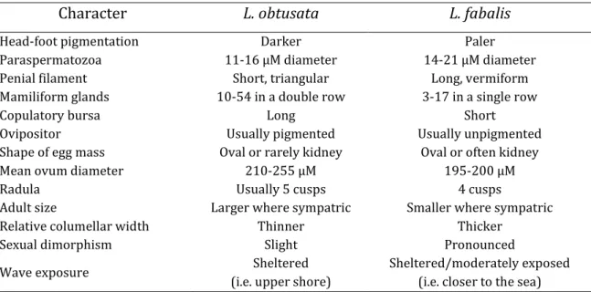
13 Despite the similarities, some important differences do exist between L. fabalis and L. obtusata (Table 1), such as their preferential location along the intertidal shore, with L. fabalis individuals commonly found in more exposed zones when compared to L. obtusata (Reid, 1996). However, many of these characters are either of subjective interpretation, difficult assessment or are not completely diagnostic but rather represent a phenotypic continuum without clear boundaries between the two species. For example, L. fabalis individuals are generally smaller and possess a more flattened shell, but the intraspecific variation is so large that shell morphology is far from being a diagnostic trait. One exception is penis morphology (Table 1, Figure 2), which constitutes one of the most used (and reliable) traits to distinguish individuals from the two species (though it does not apply to females, which are still phenotypically difficult to classify).
Table 1. Distinctive characters between Littorina obtusata and L. fabalis
Character L. obtusata L. fabalis
Head-foot pigmentation Darker Paler
Paraspermatozoa 11-16 µM diameter 14-21 µM diameter
Penial filament Short, triangular Long, vermiform
Mamiliform glands 10-54 in a double row 3-17 in a single row
Copulatory bursa Long Short
Ovipositor Usually pigmented Usually unpigmented
Shape of egg mass Oval or rarely kidney Oval or often kidney
Mean ovum diameter 210-255 µM 195-200 µM
Radula Usually 5 cusps 4 cusps
Adult size Larger where sympatric Smaller where sympatric
Relative columellar width Thinner Thicker
Sexual dimorphism Slight Pronounced
Wave exposure Sheltered
(i.e. upper shore)
Sheltered/moderately exposed (i.e. closer to the sea) Adapted from Reid (1996)
On the other hand, genetic differentiation between the flat periwinkles has been observed at several allozyme loci (Rolán-Alvarez et al., 1995), indicating that genetic tools can provide crucial information for species identification. Indeed, recently, Kemppainen et al. (2009) were able to demonstrate a clear separation between L. fabalis and L. obtusata from Northern Europe (NE) based on microsatellite loci, although they also found a lack of clear differentiation for mitochondrial DNA (mtDNA). Nonetheless, the limitations of these datasets
14 compromise the ability to make genome-wide generalizations and to accurately characterize putative hybrids between the two species.
3. Intraspecific diversification of flat periwinkles
Similarly to L. saxatilis, where several ecotypes have been described in multiple geographic regions (Butlin et al., 2014), the flat periwinkles present phenotypic variation, and in certain cases genetic variation, associated with different microhabitats (Reid, 1996; Johannesson, 2003; Kemppainen et al., 2011).
In L. obtusata, significant variations in shell size and shape have been reported across its distribution range associated to different wave-exposure conditions (Reid, 1996). However, they have not been systematically studied. In contrast, several L. fabalis ecotypes occupying different habitats and facing different regimes of wave-exposure have been the targets of several studies. In NE, two locally adapted ecotypes were identified (Figure 3). While in shores of moderate wave-exposure, individuals are bigger and have a broader shell with a relatively larger aperture (‘Large-Moderately exposed’ ecotype, LM); in more sheltered habitats, shells are smaller and present a narrower aperture (‘Small-Sheltered’ ecotype, SS)
Figure 2. Typical penis morphology of Littorina obtusata (A and C) and L. fabalis (B and D).
Note the difference in size of the penis filament and in number and arrangement of the mamiliform glands. Panels A and B are adapted from Reid (1996).
15 (Tatarenkov & Johannesson, 1999; Johannesson & Mikhailova, 2004; Kemppainen et al., 2005, 2009). Nevertheless, both ecotypes mostly dwell in the canopy of fucoid algae (mainly Fucus spp. and Ascophyllum spp.).
In the Iberian Peninsula (IP), three different ecotypes were described (Figure 4; Rolán & Templado, 1987; Williams, 1990; Lejhall, 1998; Tatarenkov & Johannesson, 1998), not only associated with different levels of wave-exposure (as the Northern ecotypes), but also with different “host” algae, although the two factors are probably correlated. In areas of intermediate wave-exposure, the ‘Fucus-Intermediate’ ecotype (FI) is characterized by medium-size snails associated with the brown algae Fucus spp.; the ‘Zostera-Sheltered’ ecotype (ZS) is found in a single location occupying an extremely sheltered habitat, where snails of larger size inhabit the green seagrass Zostera spp.; and on the most extreme wave-exposure conditions that L. fabalis can tolerate, a dwarf and red/brownish ecotype is found associated with the red algae Mastocarpus stellatus, the ‘Mastocarpus-Exposed’ ecotype (ME).
Figure 3. Large-Moderately Exposed (LM) and Small-Sheltered (SS) ecotypes of Littorina fabalis and their known distribution in Northern Europe. ANG – Anglesey; STU – Studland; RHB – Robinhoods Bay; SHE
– South Shetland; BER – Bergen (Norway), KOS – Koster (Sweden - both ecotypes have been described in various off shore islands) and WS – White Sea (Kandalaksha) (detailed locations described in Tatarenkov & Johannesson (1994) and Kemppainen et al. (2009)).
16 The association between shell and host-algae colors that is generally observed (Figure 5), probably reflects camouflage to avoid predators (Reimchen, 1979), although further studies are needed to properly test this hypothesis.
It can also be hypothesized that the smaller size and thinner shell of the ME ecotype results from an adaptation to prevent dislodgement by waves in the exposed shore where it is found, as suggested for the wave-exposed ecotypes of L.
Figure 4. Littorina fabalis ecotypes and their distribution in the Iberian Peninsula, as available at the onset of this work. The distribution of the ‘Zostera-Sheltered’ (ZS) ecotype is colored in blue; in
black, of the ‘Fucus-Intermediate’ (FI) ecotype; and in red, of the ‘Mastocarpus-Exposed’ (ME) ecotype (detailed locations from Rólan-Alvarez & Templado (1987) and Rólan-Alvarez (1995)).
Figure 5. Association between Littorina fabalis shell and host algae/seagrass colors, in the Iberian Peninsula. Note the striking resemblance between the red/brownish color of the ME ecotype (A) and the
Mastocarpus spp. algae (D), the yellow color of the FI ecotype (B) and that of the Fucus spp. algae (E), and
17 saxatilis, which, in addition to its larger foot, presents also a smaller and thinner-shell when compared to the sheltered ecotypes (Butlin et al., 2014). However, the opposite trend is observed in NE, where individuals from moderately exposed shores are larger than those living on more sheltered locations (Tatarenkov & Johannesson, 1999; Johannesson & Mikhailova, 2004). Kemppainen et al. (2005) determined that the increased risk of dislodgment in more exposed habitats creates a selective pressure for a larger size of the LM ecotype in the Swedish shores, because these individuals are able to more effectively withstand crab predation when they fall off their host algae. Although this suggests that selection on size in L. fabalis depends on a complex interaction between different factors (e.g. predation, dislodgment risk and protection by host algae).
Concerning the spatial distribution of the ecotypes, in Sweden and Norway, the LM and SS ecotypes are almost parapatric, with a continuous distribution within a range of 150 to 300 meters between the sheltered and moderately exposed extremes, meaning plenty of opportunity for gene flow among ecotypes (Figure 6); whereas in UK, despite their close geographic location (<10 Kilometers (Km)), the ecotypes tend to be allopatrically distributed (Rui Faria, pers. obs.). Although the distribution of the different L. fabalis ecotypes in the IP is allopatric (Rui Faria, pers. obs.), they are generally separated by larger distances than in UK (Figure 7). Nevertheless, regardless of their current distribution, current and/or past gene flow between the ecotypes within each country/region is not implausible.
Figure 6. Location of the moderately exposed and sheltered habitats within a single location in Sweden (Lökholmen Island). The LM and SS ecotypes of Littorina fabalis present an almost
parapatric distribution within a range of 150 to 300 meters between the sheltered and moderately exposed extremes.
18 Only a few studies have focused on the genetic differentiation between L. fabalis ecotypes and even fewer in L. obtusata (but see Schmidt et al., 2007). Evidence for a role of natural selection in the evolution of L. fabalis ecotypes comes from the discovery of an association between the different ecotypes and contrasting allelic frequencies at one allozyme locus (Arginine Kinase, ArK) detected in L. fabalis populations in two small islands of the Western coast of Sweden (Tatarenkov & Johannesson, 1994), Wales and France (Tatarenkov & Johannesson, 1999), which was recently confirmed by the finding of signatures of a selective sweep in this same gene using sequencing data (Kemppainen et al., 2011). However, the fact that similar signatures of selection in this gene were not found in the IP suggests a different genetic makeup of the L. fabalis ecotypes from this region (Tatarenkov & Johannesson, 1999), although this needs to be further studied in more detail because of the inherent problems of allozyme studies.
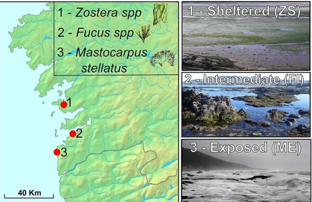
Figure 7. Location of three populations of Littorina fabalis ecotypes and respective host algae/seagrass in Galicia (Northern IP) analyzed in this study. The distribution of the ecotypes is not restricted to these
sites but we use this example to highlight their allopatric distribution, with populations separated by >25 kilometers. The algae/seagrass, level of wave exposure and ecotype (in brackets) associated with each site is indicated. Images illustrating the habitats of the different sites are also included.
19 4. Focal system and main goals
The system comprised by the flat periwinkles and their ecotypes allows the exploration of the mechanisms promoting divergence across the speciation continuum (between different ecotypes and sister species). Although natural selection is most likely playing an important role in ecotype divergence in L. fabalis, as well as in reproductive isolation between this species and L. obtusata, many of the previous studies were based on a limited number of markers of low resolution, thus lacking the necessary power to adequately tackle this question.
In order to circumvent those limitations, here I will analyze several populations of L. fabalis from NE, including the SS and LM ecotypes; and from the IP, including the ME, FI and ZS ecotypes, together with populations of L. obtusata, by means of AFLP (Amplified Fragment Length Polymorphism) and microsatellite markers, respectively, complemented by a phenotypic analysis of the shell based on geometric morphometrics. The independent genetic analysis of the two regions (the IP and NE) is justified by the differences in available information from previous studies on both regions (i.e. very limited knowledge for Iberian populations) and the split, evident at mtDNA, between Iberian and Northern European populations (Kemppainen et al., 2009; Faria et al., unpublished results), similarly to L. saxatilis (Butlin et al., 2014).
By examining different stages along the continuum of speciation (e.g. ecotypes adapted to different habitats, to different habitats and host algae and sister species), I aim to improve our understanding of the mechanisms responsible for diversification in flat periwinkles, hoping that this knowledge could be applicable to other taxa, allowing to make generalizations about the mechanisms of speciation. To achieve this main goal, three specific objectives were defined:
1. Study the phenotypic differentiation in shell size and shape between L. fabalis and L. obtusata as well as among the different L. fabalis ecotypes, developing a new geometric-morphometrics protocol specific for flat periwinkles.
20 2. Provide a new battery of polymorphic microsatellite markers specific for flat periwinkles to assess the genetic variation in populations of L. obtusata and L. fabalis (including ME, FI and ZS ecotypes) from the IP, as well as to detect putative cases of hybridization between L. obtusata and L. fabalis.
3. Perform an AFLP genome scan between LM and SS ecotypes of L. fabalis from NE to evaluate the degree of parallelism of their divergence at different geographic scales (across different countries and across locations within countries) and the proportion of the genome under divergent selection between sheltered and moderately-exposed locations.
21
Material and methods
1. Prospection of flat periwinkles in the North of Portugal
Despite several descriptions of the distribution of flat periwinkles in NE and in Galicia (Rolán & Templado, 1987; Reid, 1996; Kemppainen et al., 2011), their presence in Portugal, considered the Southern limit of the species, was basically unknown. In order to fill this gap, an initial prospection along the Portuguese coast from Caminha to Nazaré was carried out between 2011 and 2013 (see Supplementary Information).
2. Sampling
A total of 21 sites were selected for sampling, encompassing two main regions: IP and NE. Sampling methodology is described in Supplementary Information.
2.1. Sampling locations in the Iberian Peninsula
In the IP, 918 samples were collected from September 2012 to February 2013 along the Northern coast of Portugal and Galicia (Table 2, Figure 8,). Each location was classified in terms of exposure to wave action, inferred from the presence of different algae. Mastocarpus stellatus is typical of more exposed sites of the lower intertidal (locations 1, 2, 11 and 12, Table 2, Figure 8). In the other extreme, the presence of the seagrass Zostera spp. is characteristic of very sheltered locations inhabiting sandy/muddy subtracts (locations 6 and 7, Table 2, Figure 8). Meanwhile, the presence of Fucus spp. is indicative of intermediate exposure between the previous two (locations 3, 4, 5, 8 and 9, Table 2, Figure 8).
Although Moinhos (location 10, Table 2, Figure 8) is located in a very exposed shore, a barrier of rocks in the lower intertidal allows the existence of Fucus spp. in the upper (and protected) part, where L. obtusata is usually found, suggesting that the specific place where they have been collected is indeed a sheltered location. As well, although Cabo do Mundo (location 13, Table 2, Figure 8) is also wave-exposed, the specific sampling site is somehow protected by the configuration of the beach and inhabited by Fucus spp. However, it is not clear if strong wave action in winter
22 can pose important selective pressures in this locality, which was classified as unknown in order to be conservative.
Table 2. Sampling information for the IP. N is the number of sampled individuals (918 in total). Location
numbers in front of each name follow Figure 8. Putative species and ecotypes were inferred based on the type of habitat where the snails were collected and on their shell appearance (determined on site).
Location Habitat Type Sampling Date N Ecotype Putative Species
Oia (1) Exposed November 2012 24 ME L. fabalis
Silleiro (2) Exposed Oct. 2012/Feb. 2013 74 ME L. fabalis
Canido (3) Intermed. to Exposed October 2012 93 FI L. fabalis
Cangas (4) Intermediate November 2012 119 FI Mainly L. fabalis
Tirán (5) Intermediate November 2012 133 FI L. fabalis
Grove 1 (6) Sheltered December 2012 60 ZS L. fabalis
Grove 2 (7) Sheltered December 2012 23 ZS Mainly L. fabalis
Muros (8) Intermed. to Exposed December 2012 25 FI L. fabalis
Abelleira (9) Intermediate December 2012 84 FI Mainly L. fabalis
Moinhos (10) Sheltered November 2012 85 - L. obtusata
Póvoa (11) Exposed November 2012 63 ME L. fabalis
Agudela (12) Exposed November 2012 65 ME L. fabalis
Cabo do
Mundo (13) unknown November 2012 70 FI L. fabalis
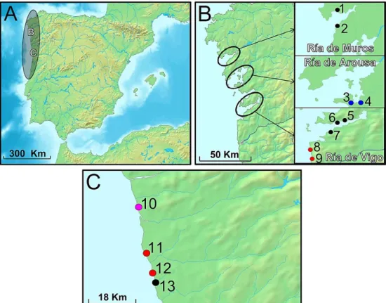
Figure 8. Sampling locations in the IP. (A) Flat periwinkles’ distribution is limited to the Northwestern shores
of the IP. (B) In Galicia, sampling locations span three main Rías: Muros e Noia, Arousa and Vigo. (C) In Portugal, sampling locations are comprised between South of Viana do Castelo and North of Porto, from top to bottom. This area covers the entire range of habitat conditions associated with L. fabalis ecotypes in the region. Point colors indicate the putative sampled ecotype: black for FI, blue for ZS and red for ME; while pink indicates a putative L.
23 2.2. Sampling locations in Northern Europe
In NE, 662 individuals were collected between August and October 2012 in Norway, Sweden and the United Kingdom (UK), from at least two locations within each country (Table 3, Figure 9). The presence of Ascophyllum spp. (besides Fucus spp.) was used as the criterion to classify these locations as sheltered, while in moderately-exposed locations only Fucus spp. was generally found (Table 3), as described in Tatarenkov and Johannesson (1998).
Within each location, a moderately-exposed and a sheltered site were sampled, with two exceptions: i) North Anglesey in UK, where the sheltered (6) and moderately-exposed (7) sites are from different locations (Table 3, Figure 9); and ii) Ursholmen (5) in Sweden where, despite the indication of the existence of one moderately-exposed and one sheltered site (Kerstin Johannesson, personal communication), the high density of Ascophyllum spp. observed in both sites rather suggests that they are both sheltered (Table 3, Figure 9). Thus, in Norway and
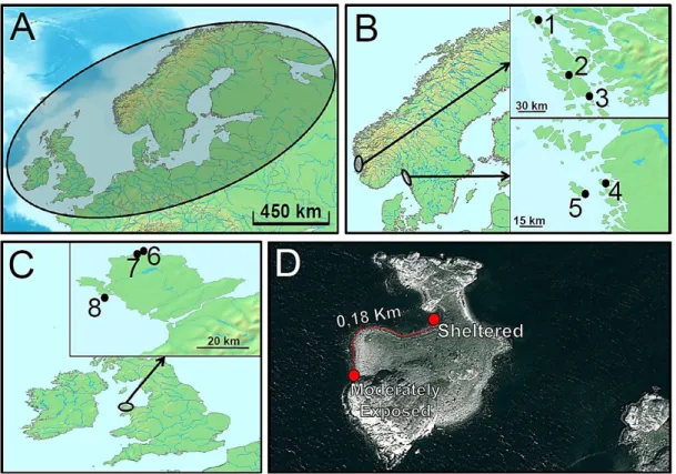
Figure 9. Sampling locations in NE. (A) Flat periwinkles are widely distributed in the North Atlantic,
occupying most coastal areas. (B) In Norway, sampling was conducted at: 1 – Sele, 2 – Syltonya and 3 – Hummelsund; and in Sweden at: 4 – Lokholmen and 5 – Ursholmen. (C) In Anglesey (UK), sampling was conducted at: 6 and 7 – Anglesey North and 8 – Anglesey South. Black dots indicate sampling locations, with numbers corresponding to those in Table 3. (D) In Norway and Sweden, moderately-exposed and sheltered sites in each location were separated by less than 1 Km, as exemplified in Lokholmen (point 4, Sweden).
24 Sweden, the sampled moderately-exposed and sheltered habitats were geographically very close to each other (<1 Km), while in UK the distance between the two habitats was larger (South Anglesey: 1.5 Km; North Anglesey: 10 Km) (Figure 9). The sampling methodology in NE is also described in Supplementary Information.
Table 3. Sampling summary for NE. Locality numbers in front of each name follow Figure 9. N is the number
of individuals sampled (662 in total, from three countries).Ecotype was inferred based on the type of habitat where the snails were collected and the abundance of Ascophyllum spp. LM, Large-moderately exposed ecotype; SS, Small-Sheltered ecotype
*Despite previous information on this site as moderately-exposed, the observed high density of Ascophyllum spp. rather suggests that it is sheltered. **In this location, the exposure could not be objectively determined. Despite presenting features compatible with a classification between intermediate and moderately-exposed, it was conservatively classified as unknown.
The protocol for sample processing is described in detail in the Supplementary Information. Briefly, individuals were sexed using the dissection microscope (Nikon SMZ1000) and males were classified into L. fabalis or L. obtusata based on the penis morphology, whereas females were classified based on their shell appearance. Nonetheless, their species status was further evaluated by means of geometric morphometrics and genetic analyses, for which shell and soft tissues were separately preserved.
Country Location Habitat Type Code Sampling Date N Ecotype
Norway Sele (1) Moderately-Exposed Sel_Exp August 2012 30 LM
Norway Sele (1) Sheltered Sel_Shl August 2012 26 SS
Norway Syltonya (2) Moderately-Exposed Syl_ExpA August 2012 30 LM
Norway Syltonya (2) Sheltered Syl_Shl August 2012 22 SS
Norway Syltonya (2) Moderately-Exposed Syl_ExpB August 2012 34 LM
Norway Hummelsund (3) Sheltered Hum_Shl August 2012 38 SS
Norway Hummelsund (3) Moderately-Exposed Hum_Exp August 2012 33 LM
Sweden Lokholmen (4) Moderately-Exposed Lok_Exp Sept./Oct. 2012 43 LM
Sweden Lokholmen (4) Sheltered Lok_Shl Sept./Oct. 2012 41 SS
Sweden Ursholmen (5) Moderately-Exposed* Urs_Exp* Sept./Oct. 2012 35 LM
Sweden Ursholmen (5) Sheltered Urs_Shl Sept./Oct. 2012 59 SS
UK Anglesey – North (6) Sheltered AngN_Shl September 2012 50 SS
UK Anglesey – North (7)
Moderately-Exposed AngN_Exp September 2012 21 LM
UK Anglesey – North (7) Intermediate AngN_Int September 2012 22 SS
UK Anglesey – North (7) Unknown** AngN_Unk** September 2012 50 LM
UK Anglesey – South (8) Sheltered AngS_Shl September 2012 56 SS
UK Anglesey – South (8)
25 3. Geometric Morphometrics analysis
In order to identify the differences in shell size and shape between groups of individuals a geometric morphometrics (GM) analysis was performed (Rohlf & Bookstein, 2003) (see Supplementary Information). Shells were positioned following the protocol developed for L. saxatilis (Carvajal-Rodríguez et al., 2005) (Figure 10) and photographed with a Nikon SMZ1500 dissection microscope. Based on a preliminary analysis, different number of landmarks (LM) and semilandmarks (SLM) were used for individuals from the IP and from NE (Figure 10, see Supplementary Information).
The software packages tpsUtil v.1.58, tpsDig v.1.40 and tpsRelw v.1.49 (http://life.bio.sunysb.edu/ee/rohlf/software.html) were used to perform the Generalized Procrustes Analysis, based on the superimposition method (Kaliontzopoulou, 2011), following the pipeline described in Figure 11. Size was studied using the centroid size (CS - defined by the squared root of the sum of the square distances of each LM and SLM to the centroid), and shape differences were subdivided into uniform (U1 and U2) and non-uniform (Relative Warps, RWs) components (see Supplementary Information).
Figure 10. Standard position in which the photographs were taken and placement of the used landmarks. (A) Iberian FI ecotype of L. fabalis with 4 LMs (blue dots) and 32 SMLs (green dots). (B) Northern
European LM ecotype of L. fabalis with 2 LMs (blue dots) and 26 SMLs (green dots). SLMs are equidistantly placed from each other and between two fixed landmarks. Each square of the grid has 1 mm sides.
26 In the IP, a total of 184 individuals (only adult males, with the species assigned based on penis morphology) were analyzed (Table 4). Additionally, individuals with shell scars, resulted from crab attacks, were also excluded. For the ME individuals from Silleiro and Oia, it was not possible to remove the soft tissues without damaging the shell. Consequently, they were only included in the genetic analysis.
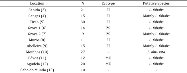
Table 4. Individuals from the IP included in the GM analysis. Location numbers after each name follow
Figure 11. N is the number of individuals analyzed for each population. In total: 92 FIs, 32 MEs, 23 ZSs and 37 L.
obtusata.
Location N Ecotype Putative Species
Canido (3) 21 FI L. fabalis
Cangas (4) 15 FI Mainly L. fabalis
Tirán (5) 30 FI L. fabalis
Grove 1 (6) 14 ZS L. fabalis
Grove 2 (7) 9 ZS Mainly L. fabalis
Muros (8) 11 FI L. fabalis
Abelleira (9) 15 FI Mainly L. fabalis
Moinhos (10) 27 - L. obtusata
Póvoa (11) 12 ME L. fabalis
Agudela (12) 20 ME L. fabalis
Cabo do Mundo (13) 10 - -
Figure 11. GM analysis pipeline. Illustrative representation of the implemented pipeline with the software
27 In NE, a total of 78 individuals (adults) were analyzed (Table 5). Since sample size in some locations was low, both males and females were included in the analyses.
Table 5. Individuals from NE included in the GM analysis. Locality numbers after each name follow Figure
12. N, number of individuals analyzed for each population. In total: 39 SSs and 39 LMs.
3.1. Data analysis
In the IP, two different analyses, i) including and ii) excluding L. obtusata individuals, were performed. To uncover significant differences in the means across ecotypes and across each ecotype and L. obtusata, we applied different statistical tests (One-way ANOVA, completed with post-hoc tests and t-tests; see Supplementary Information for details). Additionally, a PCA (Principal Component Analysis) was performed to summarize the different morphological variables (CS, U1, U2, RWs) and determine whether or not the ecotypes (and species) can be accurately distinguished based on shell morphology (see Supplementary Information). The same statistical analyses were performed in the L. fabalis ecotypes from NE. All analyses were carried out using STATISTICA v.12 (Sokal & Rohlf, 1994).
4. Genetic analysis
The genetic analysis included two main sections. Firstly, we performed a comprehensive genetic characterization of the L. fabalis ecotypes in the IP and investigated the degree of differentiation between this species and L. obtusata, identifying putative hybrids, through the development and analysis of highly variable neutral markers (microsatellites). Secondly, benefiting from the more
Country Locality Code N Ecotype
Norway Sele (1) Sel_Exp 16 LM
Norway Sele (1) Sel_Shl 8 SS
Sweden Lokholmen (4) Lok_Exp 5 LM
Sweden Lokholmen (4) Lok_Shl 14 SS
UK Anglesey – South (8) AngS_Shl 17 SS
28 extensive knowledge concerning the genetic differentiation between the L. fabalis ecotypes in NE (e.g. Tatarenkov & Johannesson, 1999; Kemppainen et al., 2009), we performed a genome scan to identify genomic regions underlying adaptive divergence between these ecotypes in different countries by means of AFLP (Amplified Fragment Length Polymorphism) markers.
4.1. DNA extraction
Genomic DNA was extracted from foot tissue using the CTAB-chloroform protocol described in Galindo et al. (2009). DNA quantity and purity were assessed with a Biophotometer (Eppendorf) and adjusted to a final concentration of 20 ng/µL for each individual.
4.2. Microsatellite analysis
In order to investigate the degree of differentiation between the Iberian L. fabalis ecotypes and between this species and L. obtusata, a battery of highly variable neutral markers (microsatellites) was developed and genotyped for the 13 populations mentioned above (Table 2).
4.2.1. Laboratorial procedures
Microsatellite loci development was performed by GENOSCREEN (Lille, France), following the protocol described by Malausa et al. (2011). Thirty-three primer pairs were selected and initially tested (see Supplementary Information), 17 of which were amplified in three multiplex PCR reactions for 344 individuals (Table 6). Each individual (20 ng of DNA) was amplified with 4 µL of QIAGEN Multiplex kit, 0.2 µM of each FAM/HEX primer pair and 0.4 µM of each NED primer pair in a final volume of 8 µL. PCR conditions comprised 15 initial minutes at 95C, followed by 30 cycles of 30 s at 94C, 90 s at 60C and 60 s at 72C, and 30 final minutes at 60C. One µL of a 1:20 dilution of each PCR product was loaded along with 0.15 µL of GeneScan 400HD ROX size standard (Applied Biosystems) on an ABI 3730 sequencer (Applied Biosystems). Capillary electrophoresis was outsourced to Stab Vida (Setúbal, Portugal).
29
Table 6. Summary of the 17 microsatellite loci used in this work. Name indicates the name of each locus
and they are grouped by multiplex reaction. Size refers to the predicted size in base pairs obtained from the enriched microsatellite libraries (see Supplementary Information). Tm F and Tm R are the melting temperatures of forward and reverse primers, respectively, for which sequences are also indicated.
Genotyping was manually performed in GeneMapper v.3.7 (Applied Biosystems). It is important to note that, to rule out potential doubts and to confirm genotyping consistency, 321 individuals (out of the total 344) were genotyped twice for all the loci. The EKKY locus revealed genotyping ambiguities, due to the amplification of multiple peaks in some populations, and it was consequently removed from further analyses. The DAEH locus failed to amplify in L. obtusata, but it was maintained in the analysis of genetic variability/differentiation within L. fabalis. In addition, because of the difficulties in objectively genotype the 193Q locus in Agudela, Oia, Silleiro and Grove 2, all these individuals were coded as missing data for this locus. 4.2.2. Data analysis
Hardy-Weinberg equilibrium (HWE) for each population/locus pair and linkage disequilibrium (LD) between locus pairs for all populations were evaluated through exact probability tests in GENEPOP v.4.2 (Rousset, 2008), using a Markov Chain (MC) algorithm with default parameters. A Bonferroni correction (Rice, 1989) was subsequently applied to account for multiple tests. Significant
Hardy-Name Size Tm F Tm R Forward primer (5’-3’) Reverse primer (5’-3’) Multiplex 1
PBL8 197 60 62 CCCAGACAATGCAGCCTAC CGGTAACTGAGTTGTGCAGC
QVOM 117 62 62 ACATGGGATACGACTACCCG AGCCTAGCTGCTACGTCCAA
193Q 215 62 58 TTTGCATACACCCGTCTAACC GCTATTTCATTAAGCCGCCA
KJ2E 245 62 60 TCACTTACCTCAAACCTTGCG CCACAGGCGGGGTGTAAG
VPVX 198 58 58 CGCTACGCCACTTCGTTTA AATCGGAGAACAAAACCACG
881 316 58 62 ACGCCCAGAATTGCCTAAAT GCTTGTTTATTGACAGGCAGC
Multiplex 2
EKYY 145 60 60 TTGTCAAGAATGTTGGTTCCC ATCCGGAATCGACAAGTGAC
XENN 242 58 58 CAGCACAAGGCGGTTCAG TCCTATTTGAAGATGCGGTG
ZIBW 96 58 58 TTTTGTTAACACGTGGCAGTT TTGGTGAGTGCGTGCATTAT
LHYM 192 62 58 TGGTACGGACGAGGCTCTTA ATTGCTTGAATGCCCGTTAC
927 241 62 62 CATACAATCCGTCCCTCTCC TACTCGAACAGGAACGAGGC
1871 105 60 60 CACCCACCCCTATTACCCA GGGTTGATGGATGAGTGGAT
Multiplex 3
DAEH 242 60 60 ACCGCACAGCTACACGAAG TCGTGTTTCATGATGCCCTAT
47 194 62 62 TGTTGCTCTGCAGATTATGACA GATCGATGCCCTGACATAGC
EVLS 112 58 62 GTTTTGGTTGAATGTTGGGC GACAGAAAACAGAAACAACGAAA
TEM7 237 60 60 CTCATGCTGTTCCTGGTTGA TGCGTGGTTTAAATTGTTCTTG
30 Weinberg disequilibria were further inspected to distinguish between possible genotyping errors (null alleles, stuttering and large allele dropout) using MICRO-CHECKER v.2.2.3 (van Oosterhout et al., 2004).
Genetic diversity was evaluated through several parameters. Average expected (He), observed (Hobs) and non-biased heterozygosity (Hnb); percentage of polymorphic loci, either taking 1% (P99) or 5% (P95) as the minimum allelic frequency to consider an allele as a true polymorphism rather than an artifact; and mean number of alleles per locus (A) for each population were estimated using GENETIX v.4.05 (Belkhir et al., 1996). Mean allelic richness (Ar) and private allelic richness (PAr) were estimated using the rarefaction method implemented in HP-Rare v.1.1 (Kalinowski, 2005). Since PAr of a given population does not only depends on its own genetic variability but also on the diversity of the other populations in the dataset, and since the number of populations analyzed for L. fabalis and L. obtusata differs considerably (two vs. 11), PAr was separately calculated for each species.
Population structure was investigated using the Bayesian clustering method implemented in STRUCTURE v.2.3.4 (Falush et al., 2007). Two separate analyses were performed. First, to inspect the differences between L. fabalis and L. obtusata, as well as the presence of putative hybrids, information from all genotyped individuals was included for 14 loci (besides the EKKY, 193Q and DAEH were removed to avoid distorted estimates of hybridization/introgression due to null alleles), with the number of clusters (K) ranging from 1 to 13 (the total number of locations sampled). Second, to assess the genetic substructure within L. fabalis, STRUCTURE was run including only the individuals we were certain of being true L. fabalis (using penis morphology – males, and information from the previous STRUCTURE run - males and females). In this case, the genotypes for 15 loci were included (besides the EKKY, the 193Q was removed due to the existence of null alleles in L. fabalis), and 1 to 11 (the total number of L. fabalis sampled locations) clusters (K) were considered. For the two analyses, ten replicate runs were performed for each K, with 10,000,000 iterations (100,000 as burn-in), assuming
31 an admixture model, correlated allele frequencies and without population prior information.
The method of Evanno et al. (2005), implemented in STRUCTURE HARVESTER (Earl & vonHoldt, 2012), was then employed to determine the K that best fitted the data. The results from the multiple replicates of the best K value were combined using the Greedy algorithm in CLUMPP v.1.1.2 (Jakobsson & Rosenberg, 2007) and the obtained output was plotted using DISTRUCT v.1.1 (Rosenberg, 2004). For the L. fabalis dataset, we also used an empirical approach as suggested in the STRUCTURE manual (http://pritch.bsd.uchicago.edu/structure.html), which defines the best K as the highest among those with a similarly high posterior probability, in which at least one individual is strongly assigned to each cluster (Q>80).
Differentiation between populations was also assessed by means of FST (Weir & Cockerham, 1984) and RST (Slatkin, 1995) between all population pairs using FSTAT v.2.9.3.2 (Goudet, 1995) and GENEPOP, respectively. The correlation between pairwise FST and RST was tested by means of a Spearman’s Rank Correlation Coefficient (Sokal & Rohlf, 1994). Average differentiation between species and ecotypes was estimated as the mean of all pairwise values including populations from the two species or from each pair of ecotypes, respectively. The correlation between genetic and geographic distance, i.e. isolation by distance (IBD), among L. fabalis populations was tested by means of a Mantel test (Mantel, 1967), and its significance obtained with 10,000 permutations, using GENEPOP. Both FST as well as transformed values of differentiation using Slatkin’s (1995) linearized FST (FST/(1-FST)) were used. Geographic distances between sampling locations were calculated as the shortest distance along the coast according to Google Maps (https://maps.google.com/), with both linear and log transformation of the geographic distances tested against genetic distances. A second analysis of IBD in L. fabalis was performed after excluding ME populations, which seem to be affected by stronger drift than the populations from the remaining ecotypes (see Discussion).
32 Neighbor-joining (NJ, Saitou & Nei, 1987) trees (population- and individual-based) were constructed based on Nei’s DA distance (Nei et al., 1983) in POPULATIONS v.1.2.31 (http://www.cnrs-gif.fr/pge/bioinfo/liste/index.php?lange=fr), with node support estimated through 1000 bootstrap replicates (over loci). FIGTREE v.1.4.0 (http://tree.bio.ed.ac.uk/software/figtree/) was used to visualize the trees.
4.3. AFLP analysis
The detection of loci under selection (i.e. outlier loci) by means of AFLP genome scans is a widespread methodology in studies of adaptation and speciation (Nosil et al., 2009a; Butlin, 2010) and it has been successfully applied to different populations within the genus Littorina (Wilding et al., 2001; Galindo et al., 2009, 2013; Butlin et al., 2014). Loci are classified as “outliers” when they exhibit significantly greater genetic differentiation (i.e. FST) than neutral expectations (obtained through simulations); otherwise they are classified as “nonoutliers”. Here, we performed a genome scan using AFLPs to investigate the level of divergence between L. fabalis ecotypes in NE (Norway, Sweden and the UK) and to identify putative loci underlying ecotype divergence between sheltered and moderately-exposed habitats, as well as the degree of parallelism in such divergence (i.e. proportion of outlier loci shared) at different scales (within country and among countries).
4.3.1. Laboratorial procedures
The general AFLP protocol comprises four main steps: i) digestion with two restriction enzymes (a 4 bp and a 6 bp cutter), ii) ligation with double-stranded adapters complementary to the restriction enzymes’ recognition sites, iii) pre-selective PCR with primers containing one pre-selective nucleotide on the 3’ end, and iv) selective PCR with primers containing three selective nucleotides (Vos et al., 1995). Here, we applied the specific protocol developed for L. saxatilis by Butlin et al. (2014), with minor modifications (see Supplementary Information), among which, I would like to highlight the use of EcoRI (6 bp) and MseI (4 bp) restriction enzymes because according to other L. saxatilis studies (Galindo et al., 2009;
33 Galindo et al., 2013), they allow more loci to be genotyped when compared to the combination used by Butlin et al. (2014) (EcoRI (6 bp) and PstI (6 bp).
Four selective PCRs (Eco+ACT/Mse+CAA; Eco+AAG/Mse+CAA;
Eco+ACT/Mse+CAC; Eco+AAG/Mse+CAC; see Supplementary Information) were performed in a total of 379 individuals from seven localities across three countries. For each selective PCR, 0.8 µL were analyzed on an ABI3130 sequencer (Applied Biosystems) along with 0.2 µL of GeneScan 500ROX size standard (Applied Biosystems). Electropherograms were analyzed with GeneMapper v.3.7. Loci were manually assigned by defining bins (fragment-length classes) from the overlapping electropherograms of all the samples. Bins were created between 75 and 500 bp and only peaks >50 rfu (relative fluorescent units) were considered. For each sample, fluorescence intensity of the peaks (peak height) within each bin was also determined. This step was repeated for each of the four primer combinations (selective PCRs). The R-script AFLPSCORE (Whitlock et al., 2008) was used to transform peak heights into binary (0/1) genotype data based on quality thresholds (locus selection and phenotype-calling thresholds) determined from the data of replicated samples. AFLPSCORE was also used to estimate the mismatch error rate by comparing the dissimilarity between sample replicates for each combination (Whitlock et al., 2008).
4.3.2. Data analysis
Based on all genotyped AFLP loci, heterozygosity and percentage of polymorphic loci, taking 5% (P95) as the minimum allelic frequency to consider an allele as a true polymorphism, were calculated using AFLP-SURV v.1.0 (Vekemans et al., 2002). The same software was used to calculate genetic differentiation (FST) and Nei’s genetic distances (D), following Lynch & Milligan (1994), using a Bayesian method that assumes a non-uniform prior distribution of allele frequencies (Zhivotovsky, 1999).
The detection of loci under selection (outlier loci) between moderately-exposed and sheltered sites was then performed in an independent manner within each
34 locality: Hum_Exp/Hum_Shl; Sel_Exp/Sel_Shl; Syl_ExpA/Syl_Shl; Lok_Exp/Lok_Shl; AngN_Exp/AngN_Shl; AngS_Exp/AngS_Shl; as well as Urs_Exp*/Urs_Shl, despite the doubts concerning the exposure in Urs_Exp (Table 3). In Syltonya (Norway), because two exposed locations were sampled, we selected the most exposed one (Syl_ExpA) for outlier detection.
The outlier detection was performed applying the two most commonly used methods in the literature (Pérez-Figueroa et al., 2010): BAYESCAN v.2.0 (Foll & Gaggiotti, 2008) and MCHEZA (Antao & Beaumont, 2011), more and less stringent, respectively.
BAYESCAN first calculates population-specific and locus-specific FST, and then estimates the posterior probabilities of two alternative models (including or excluding the effect of selection) for each locus using a reversible-jump Markov Chain Monte Carlo (MCMC) approach. Ten pilot runs (10,000 iterations) were performed to tune the model parameters, followed by 400,000 iterations (100,000 as burn-in, 20 as thinning interval and 20,000 as sample size). Loci were identified as outliers when the posterior probability was greater than 0.97, but a correction for multiple tests (false discovery rate - FDR; Benjamini & Hochberg, 1995) was applied to avoid overestimating the proportion of loci that are under divergent selection.
MCHEZA is adapted from the DFDIST program
(http://www.maths.bris.ac.uk/~mamab/stuff/), which is based on the method developed by Beaumont and Nichols (1996). The program generates loci obtained through coalescent simulations using a neutral model with two symmetrical islands. Then, the distribution (FST conditional on heterozygosity) of simulated loci is compared to the empirical data and loci with FST significantly greater (p<0.05) than the simulated FST are classified as outliers. The main advantage of MCHEZA compared to DFDIST is that it allows the estimation of the mean neutral FST while taking into account loci that might be under selection. MCHEZA also introduces support for multi-test correction (FDR method) to reduce the number of false positives. For each locality, 200,000 simulations were performed, with a theta of