Gonçalo Miguel Grenho Rodrigues
Bachelor Degree in Biomedical Engineering SciencesReal-Time Step Detection Using Unconstrained
Smartphone
Dissertation submitted in partial fulfillment of the requirements for the degree of
Master of Science in Biomedical Engineering
Adviser: Hugo Filipe Silveira Gamboa, Professor Auxiliar, Faculdade de Ciências e Tecnologia, Universidade NOVA de Lisboa
Real-Time Step Detection Using Unconstrained Smartphone
Copyright © Gonçalo Miguel Grenho Rodrigues, Faculty of Sciences and Technology, NOVA University Lisbon.
The Faculty of Sciences and Technology and the NOVA University Lisbon have the right, perpetual and without geographical boundaries, to file and publish this dissertation through printed copies reproduced on paper or on digital form, or by any other means known or that may be invented, and to disseminate through scientific repositories and admit its copying and distribution for non-commercial, educational or research purposes, as long as credit is given to the author and editor.
This document was created using the (pdf)LATEX processor, based in the “novathesis” template[1], developed at the Dep. Informática of FCT-NOVA [2].
Ac k n o w l e d g e m e n t s
Without the support of many important people, I would not have been able to reach this important accomplishment in my academic and personal life.
First of all, I would like to thank Professor Hugo Gamboa for accepting me as his master thesis student and for allowing me to develop and work on this project, to develop myself and become a better Biomedical Engineer.
To Ricardo Leonardo, who support me through the whole development of my master thesis project, guiding and helping me every step of the way, I would like to express my deepest gratitude. I would’ve never been able to achieve and learn as much as I did without your support and knowledge and I’m really grateful for having you as my mentor. Thank you for all the support and patience invested in guiding me.
ToAssociação Fraunhofer Portugal Research, I would like to thank you for giving me
everything I could possibly need, for all the support provided and specially for welcoming me into the company in the best possible way.
To BEST Almada, my home away from home where I grew, learned, discovered and developed an European mindset, knowledge, skills and, specially, friendships which I will carry with me for the rest of my life. I would like to thank all of the organization and specially the other 4 Sailors with whom I’ve been having the honor and pleasure of leading the organization with.
I want to thank my family, who have supported me and helped me deal with the hardships and frustrations which came along this path to become a Biomedical Engineer. My parents and my sister for all being there when I needed, for listening, for advising and for steering me towards success. I want to thank my grandfather, who always supported and motivated me endlessly to work harder and harder every day. Thank you for making all for making me the man I am today.
I want to thank my childhood friends, with whom I’ve been going through the chal-lenges of university life and who have been with me every step of the way for the past decades. To the friends I made in FCT NOVA, who were always present, supported me and taught me many lessons in life, who spent many days and many nights besides me studying in VII or anywhere else, and helped me get through the toughest situations. To Sofia Gomes, who was there to listen to all the challenges I encountered and for guiding me towards the best path, either in life or work, and allowing me to become a person a better person every step of the way.
"The moment you accept total responsibility for everything in your life is the day you claim the power the change anything in your life." - Hal Elrod
A b s t r a c t
Nowadays smartphones are carrying more and more sensors among which are inertial sensors. These devices provide information about the movement and forces acting on the device, but they can also provide information about the movement of the user. Step detection is at the core of many smartphone applications such as indoor location, virtual reality, health and activity monitoring, and some of these require high levels of precision.
Current state of the art step detection methods rely heavily in the prediction of the movements performed by the user and the smartphone or on methods of activity recog-nition for parameter tuning. These methods are limited by the number of situations the researchers can predict and do not consider false positive situations which occur in daily living such as jumps or stationary movements, which in turn will contribute to lower performances.
In this thesis, a novel unconstrained smartphone step detection method is proposed using Convolutional Neural Networks. The model utilizes the data from the accelerome-ter and gyroscope of the smartphone for step detection. For the training of the model, a data set containing step and false step situations was built with a total of 4 smartphone placements, 5 step activities and 2 false step activities. The model was tested using the data from a volunteer which it has not previously seen.
The proposed model achieved an overall recall of 89.87% and an overall precision of 87.90%, while being able to distinguish step and non-step situations. The model also revealed little difference between the performance in different smartphone placements, indicating a strong capability towards unconstrained use. The proposed solution demon-strates more versatility than state of the art alternatives, by presenting comparable results without the need of parameter tuning or adjustments for the smartphone use case, poten-tially allowing for better performances in free living scenarios.
Keywords: Step Detection, Smartphone Sensors, Convolutional Neural Networks, Artifi-cial Intelligence, Deep Learning
R e s u m o
Atualmente, os smartphones contêm cada vez mais sensores incorporados, entre os quais temos os sensores inerciais. Estes sensores fornecem informações sobre o movi-mento e as forças que atuam no dispositivo, mas também podem fornecer informações sobre o movimento do utilizador. A deteção de passos está na base de muitas aplica-ções para smartphones, como localização indoor, realidade virtual, análise de saúde e atividade, e algumas dessas aplicações exigem altos níveis de precisão.
Os métodos de deteção de passos existentes dependem muito da previsão dos movi-mentos executados pelo utilizador e pelo smartphone ou em métodos de reconhecimento de atividade, para ajuste de parâmetros. Estes métodos são limitados pelo número de situações que os investigadores conseguem prever e não consideram situações de falsos positivos que ocorrem na vida diária, como saltos ou movimentos estacionários.
Nesta dissertação, um novo método de deteção de passos sem restrições para smartpho-nes é proposto usando Redes Neuronais Convolucionais. O modelo utiliza os dados do acelerómetro e do giroscópio do smartphone para deteção de passos. Para o treino do modelo, um data set contendo situações de passos e de falsos passos foi construído com um total de 4 colocações do smartphone, 5 atividades de passos e 2 atividades de falsos passos. O modelo foi testado usando os dados de um voluntário, que não foram sido incluídos no treino.
O modelo proposto alcançou uma recall de 89,87 % e uma precisão de 87,90 %, além de conseguir distinguir situações de passos e de falsos passos. O modelo também reve-lou pouca diferença entre o desempenho em diferentes posicionamentos do smartphone, indicando uma forte capacidade de uso irrestrito. A solução proposta demonstra mais versatilidade do que as alternativas existentes, apresentando resultados comparáveis sem a necessidade de ajustes de parâmetros para diferentes colocações do smartphone, poten-cialmente permitindo melhores desempenhos na normal utilização diária.
Palavras-chave: Detecção de Passos, Sensores Inerciais, Smartphone, Redes Neuronais convolucionais, Inteligência Artificial, Deep Learning
C o n t e n t s
List of Figures xvii
List of Tables xix
Acronyms xxi
1 Introduction 1
1.1 Contextualization . . . 1
1.1.1 Applications . . . 2
1.2 State Of The Art . . . 2
1.2.1 Parameter Based Methods . . . 3
1.2.2 Machine Learning Methods . . . 4
1.2.3 Deep Learning Methods . . . 4
1.2.4 Discussion . . . 5 1.3 Objectives . . . 5 1.4 Thesis Overview . . . 5 2 Theoretical Background 7 2.1 Sensors . . . 7 2.1.1 Accelerometer . . . 7 2.1.2 Gyroscope . . . 8 2.1.3 Magnetometer . . . 8 2.2 Gait Analysis . . . 8 2.3 Quaternions . . . 10 2.3.1 Quaternion Rotation . . . 11 2.4 Sensor Fusion . . . 12 2.4.1 Complementary Filter . . . 12 2.4.2 Reference Frame . . . 12 2.5 Machine Learning . . . 15 2.5.1 Supervised Learning . . . 15 2.5.2 Semi-supervised Learning . . . 15 2.5.3 Unsupervised Learning . . . 15 2.5.4 Reinforcement Learning . . . 15
2.5.5 Evaluation Metrics . . . 16
2.5.6 Data Sets . . . 17
2.6 Artificial Neural Networks . . . 17
2.6.1 Activation Functions . . . 18 2.6.2 Loss/Cost Function . . . 20 2.6.3 Backpropagation . . . 21 2.6.4 Network Optimization . . . 24 2.6.5 Network Regularization . . . 25 2.6.6 Types of ANNs . . . 27 3 Data Acquisition 31 3.1 Sensors Acquired . . . 31
3.2 Indoor Data Acquisition . . . 32
3.2.1 Sensor Placement . . . 33
3.2.2 Recorded Activities . . . 33
3.2.3 Indoor Route . . . 34
3.3 Free Living Data Acquisition . . . 34
3.4 Final Data Set . . . 35
3.4.1 Pandlet Disconnections . . . 35
3.4.2 Temporal Issues . . . 35
3.4.3 Heading Estimation Issues . . . 36
3.4.4 Employed Data for Training and Testing . . . 36
4 Proposed Algorithm 39 4.1 Ground Truth Extraction . . . 40
4.1.1 Final Ground Truth Algorithm . . . 41
4.1.2 Manual Corrections . . . 44
4.2 Deep Convolutional Neural Network . . . 45
4.2.1 Data Pre-processing . . . 45
4.2.2 Deep Learning Network Model . . . 48
4.3 Post processing . . . 49 4.3.1 Peak Detection . . . 49 4.3.2 Movement Vector . . . 49 5 Results 51 5.1 Metrics . . . 51 5.2 Algorithm Results . . . 52 5.3 Discussion . . . 54
6 Conclusion and Future Considerations 57 6.1 Conclusion . . . 57
C O N T E N T S
Bibliography 61
A Additional Deep Learning Results 65
L i s t o f F i g u r e s
2.1 Gait cycle temporal division. . . 8
2.2 Gait cycle Rancho classification. . . 10
2.3 Quaternion Rotation . . . 11
2.4 Smartphone reference system. . . 13
2.5 Earth coordinates reference system. . . 14
2.6 User reference system. . . 14
2.7 Linear activation function . . . 18
2.8 Sigmoid activation function . . . 19
2.9 Rectified Linear Unit (ReLU) . . . 19
2.10 Impact of the neuron on the loss value . . . 23
2.11 Dropout regularization technique. . . 26
2.12 Fully connected neural network representation. . . 27
2.13 Recurrent neural network representation. . . 28
2.14 Convolution operation. . . 29
2.15 Max pooling operation. . . 29
2.16 1D Convolution. . . 30
3.1 Fraunhofer AICOS Pandlet . . . 32
3.2 Fraunhofer AICOS Recorder App. . . 32
3.3 Signal segmentation by activity. . . 34
4.1 Step detection for unconstrained smartphones algorithm diagram. . . 39
4.2 Pandlets accelerometer signal. . . 40
4.3 Pandlets gyroscope signal. . . 40
4.4 Final ground truth algorithm representation. . . 41
4.5 Moving averages application visual representation. . . 43
4.6 Dual Pandlet peak filtering. . . 44
4.7 Ground truth binarization. . . 47
4.8 Final model for step detection. . . 48
4.9 Pedestrian’s movement peak filtering . . . 50
L i s t o f Ta b l e s
5.1 Algorithm results for each type of user movement. . . 53
5.2 Algorithm results for each smartphone placement. . . 53
5.3 Algorithm results for the entire testing data set. . . 53
5.4 Results of the proposed and analysed steps detection solutions. . . 54
5.5 Total detected steps by the analysed solutions. . . 54
A.1 Results for each activity with the Texting smartphone placement. . . 65
A.2 Results for each activity with the Right Pocket smartphone placement. . . 65
A.3 Results for each activity with the Back Pocket smartphone placement. . . 65
A.4 Results for each activity with the Jacket smartphone placement. . . 66
A.5 Recall values of the proposed model and the models proposed by Leeet al. and Edelet al. for the different activities analysed. . . 66
A.6 Precision values of the proposed model and the models proposed by Leeet al. and Edelet al. for the different activities analysed. . . 66
A.7 F-Score values of the proposed model and the models proposed by Leeet al. and Edelet al. for the different activities analysed. . . 66
A.8 Recall values of the proposed model and the models proposed by Leeet al. and Edelet al. for the different smartphone placements analysed. . . 67
A.9 Precision values of the proposed model and the models proposed by Leeet al. and Edelet al. for the different smartphone placements analysed. . . 67
A.10 F-Score values of the proposed model and the models proposed by Leeet al. and Edelet al. for the different smartphone placements analysed. . . 67
Ac r o n y m s
ACC Accelerometer.
ANN Artificial Neural Network.
BLSTM-RNN Bidirectional Long Short Term Memory-Recurrent Neural Network. CNN Convolutional Neural Network.
DL Deep Learning.
GC Gait Cycle.
GT Ground Truth.
GYR Gyroscope.
IMU Inertial Measurement Unit. LSTM Long Short Term Memory.
MAG Magnetometer.
ML Machine Learning.
PDR Pedestrian Dead Reckoning. ReLU Rectified Linear Unit. RNN Recurrent Neural Network.
SDG Stochastic Gradient Descent. SLE Step Length Estimation. SSL Semi Supervised Learning. SVM Support Vector Machine. Tanh Hyperbolic Tangent.
C
h
a
p
t
e
r
1
I n t r o d u c t i o n
1.1
Contextualization
Microelectromechanical systems (MEMS) have seen a rapid development and are now present in many of ubiquitous everyday devices such as smartphones. MEMS sensors such as accelerometers, gyroscopes and magnetometers, which constitute an Inertial Measurement Unit (IMU), can give us information about the position, orientation and the overall movement of the device and indirectly, of the user as well. These IMUs have been proven to be a reliable and cheap alternative to laboratory/industrial grade sensors [1, 2] and researchers have been using them in a wide number of fields of study, among which we have stride detection.
With this new and more accessible option, novel walk detection techniques have emerged in an attempt to correctly record the human gait. However, most of the ap-proaches taken have been limited in some aspects such as constrained positioning of the device, the lack of detection of changes of pace, which in a free living situation cause them to fail to perform with high accuracy due to the high number of variables and chal-lenges we encounter in our daily life when we are walking. Some applications of stride detection such as indoor location or gait analysis, require high accuracy and real-time use and current state of the art methods also lack the ability to accurately detect the moment of the step in real-time in some cases. As such, it has become increasingly necessary to find new solutions.
With this work, we propose a step detection algorithm that focus on improving ex-isting smartphone-based step detection by making it impervious to errors derived from different device placements on the body, changes in user movement and false step sit-uations and ensuring the correct functioning in real-time. These improvements will enhance the performance of many applications with step detection at their core, such as
indoor positioning or activity monitoring systems.
1.1.1 Applications
• Medical Gait Analysis
The use of IMU in the study of gait parameters has seen extensive research and applications [3–6]. The study of the human gait is most of the times limited to hospitals or researches centers, where laboratory grade sensors are available. How-ever, the analysis is most of the time limited to the daily life situations the medical professionals can recreate.
F. Proessla et al. [1] extracted gait parameters using a smart device attached to
the patient’s ankle. The gait parameters were extracted using peak detection in the accelerometer signal. These parameters showed high correlation with results from a validated medical sensor, the APDM Opal. Robust step detection with our everyday smartphone will allow medical professionals to study the patients gait, in free living situations where we encounter the most variability of movements and obstacles, and make better informed diagnosis.
• Indoor Location
Step detection is a major part of step detection algorithms using Pedestrian Dead Reckoning (PDR) [7–11]. PDR is one method used for indoor location where the step length and heading of the user are extracted from the IMU data and used to predict the movement in space. In order to have a high localization accuracy it is necessary to have little to no step misdetection. Accurate indoor location using a smartphone allow for inexpensive location capabilities that can be applied in emergency services, augmented reality, geofencing, worker location in factories or hospitals and as alternative for GPS location services.
1.2
State Of The Art
Over the last decades, many methods have appeared trying to record and analyse the human gait. Video recording of patients walking, force plate measurements, IMUs and other wearable sensors [5] have been employed to the study of human locomotion. With the appearance of smartphones with embedded IMUs, many researchers started to use them in this study and also found new ways of applying this knowledge of the human gait. Step counters and activity monitoring systems are now some of the most common appli-cations we find on our smartphones. The lack of accuracy indoors of GPS location also prompted researchers to look for alternatives for indoor location and found smartphones sensors to be a reliable alternative [7–16]. Nowadays, more and more applications need highly accurate and mobile step detection systems. As algorithms with step detection in
1 . 2 . S TAT E O F T H E A R T
their core continue to grow in complexity, it has become detrimental that these become more precise in order to reduce cumulative errors.
We chose to divide current state of the art algorithms in three main categories, based on the methods used, which are parameter based methods, machine learning methods and deep learning methods.
1.2.1 Parameter Based Methods
One of the most experimented approach are the parameter based methods. These use methods such as Peak and Valley Detection [7, 12, 17], Zero Crossing [18] and Short Term Fourier Transform (STFT) [19] which require manual tuning of the parameters in order to get optimal results. Lee et al. [17] proposed to solve the day to day walking
variability through a peak and valley detection method with adaptive thresholds. Using the accelerometer signal, the peak and valley detection thresholds are update using the distance in time and the magnitude of the last pair of peak and valley. Using this method, an average accuracy of 99.3% was obtained for a combination of 7 smartphone placements and 3 manners of walking. Pouloseet al. [7] used a different approach. They applied a
sensor fusion algorithm in order to obtain pitch-based step detection algorithm. Then a peak and valley detection was made with temporal and magnitude thresholds. This approach was able to produce a 3,14% error rate. This step detection method was only tested for walking and handheld position. Khedr and El-Sheimy [12] applied peak and valley detection to the acceleration norm to perform step detection. A verification of the detected peaks and valleys was also done using the magnetometer and gyroscope signal in order to compensate variations in the amplitude and frequency of the signal caused by shifts in the user movements speed and smartphone movement. An accuracy of 99.5% was achieved in free walking manner where the smartphone position and the user speed vary. This method provided a more extensive step detection solution with a wide number of walking manners and smartphone positions.
These methods provide a good estimate at step detection but they are limited by the number of positions and movements the researchers can predict. Situations such as climbing up and down stairs and false step situations were not accounted for and they can result in an increase of the error of the algorithms. Also, errors resulting from the changes in position of the smartphone and of the users movement speed are not accounted for. As a possible solution, Kanget al. [19] proposed a frequency based algorithm for walk
detection and step counting. They adaptively select the most sensitive axis of the gyro-scope and extract the most prominent frequency of the users movement using a sliding time window and Fast Fourier Transform. The steps are then counted by multiplying the frequency with the elapsed time. This proposed algorithm exhibits a good perfor-mance, with a 95,76% accuracy, and is able to distinguish between walking a non walking activities such as standing and typing.
1.2.2 Machine Learning Methods
Many approaches join the conventional parameter based methods with classification methods such as Support Vector Machines(SVMs) [8, 9, 13], Artificial Neural Networks (ANNs) [10] and Decision Trees [20] in order to increase accuracy and reduce misclassifi-cation errors.
Support Vector Machines are often used in device pose recognition and user move-ment classification due to its high performance [8]. Parket al. [13] proposed an algorithm
for walk detection using a SVM. The SVM is used to detect the placement of the de-vice by selecting features from the obtained tri-axial accelerometer and gyroscope data, increasing the accuracy of the step counting procedure. The SVM exhibited an over-all accuracy of 97.32% in device placement detection and the step detection showed a 97.09% overall accuracy. Zhanget al. [8] designed a step counting algorithm supported
by a step mode and device pose detection. Two classifiers were used for device pose and step mode recognition, a Artificial Neural Network (ANN) and a SVM. The result of the classifiers will influence the cut-off frequencies of a band pass filter in place to prevent undercounting and overcounting. This method is able to detect step with an accuracy of 98%. Rodríguezet al. [9] developed a peak and valley step supported by an ensemble
of Support Vector Machines and a Bayesian step mode probability. The support vectors machines and Bayesian probability worked together to produce coherent and correct step mode classification and reduce false classification of strides.
Liu et al. [10] proposed a step detection method using a feed forward ANN. The
proposed solution uses 5 layers and a tanh activation function with Stochastic Gradient Descent (SGD) optimizer. The ANN was able to almost perfectly detect the users steps. The ANN was tested in three different data sets, belonging to the signals of three different individuals walking a total of 80 steps. The ANN results only exhibited one false positive on the third data set and managed to count the exact number of steps correctly in the other two. This shows the applicability of ANNs for step detection, however the proposed method only tested for walking procedure and in a limited manner.
1.2.3 Deep Learning Methods
Deep Learning has risen in importance in the last few years due to its capacity to learn from the data without the need of manually defining parameters and thresholds and its versatility to many different areas of study [21–26].
In step detection and step length estimation for Pedestrian Dead Reckoning (PDR), Edel and Koppe [14] implemented a Bidirection Long Short Term Memory-Recurrent Neural Network (BLSTM-RNN). The model is able to work with the raw data of the smartphones IMU. Using this implementation they were able to obtain a high step detec-tion accuracy (1.48% mean error) for several smartphone placements and walk manners. This approach however does not take into account false step situations and other walk-ing activities such as climbwalk-ing stairs, which often compromises the accuracy of the step
1 . 3 . O B J E C T I V E S
detection. Also, a BLSTM-RNN makes real-time implementation not possible.
Steinmetzeret al. [3] proposed a novel step detection method using an insole with
sen-sors and Convolutional Neural Networks (CNNs) to detect and compare steps of healthy patients and patients with Parkinson Disease. The proposed model used 2 convolutional layers with a Rectified Linear Unit (ReLU) activation function, 2 max pooling layers and 1 dense layer in the end with sigmoid function in order for the output of the model to be a step probability. The network was able to detect the steps and return the beginning and end marks of the steps with an F1-score of 0.974 for daily living activities and 0.939 for the healthy patients and 0.938 for Parkinson Disease patients F1-score in the Time Up and Go Test.
1.2.4 Discussion
As seen, a large variety of different approaches and techniques have been employed in the past in an attempted to detect steps of the smartphone user. However, most algorithms focuses on specific tasks and movements, making adjustments in order to increased the accuracy in those cases. During an ordinary day, a person walks, runs, walks upstairs, downstairs, and makes a series of different other movements which can’t all be predicted and adjusted to, in order to have the highest accuracy possible. In these scenarios step detection algorithms which focuses on specific tasks and smartphone placements will have a lower performance and in application such as indoor location or medical moni-toring application, this can have a negative effect. As such, a real-time solution which can correctly detect each step with high accuracy and also dismiss false step situations is needed.
1.3
Objectives
With this work we propose a novel step detection method which can perform with high accuracy in free living situations and regardless of the device pose. We aim to make the automatic step detection proposal impervious to false step situations and other variables encountered in day to day situations which can be applied for real-time use. This in turn, will allow for better and more accurate applications such as indoor location which requires high accuracy of step detection and reduce cumulative errors.
1.4
Thesis Overview
This thesis contains 6 Chapters. The first chapter includes all the contextualization, state of the art and objectives of the dissertation. In the second chapter, all the theoretical concepts necessary to understand the work develop are explained. In the third chapter, an explanation of the data collection procedure for the training and testing of the proposed model is presented. In the fourth chapter, the data pre-processing and the final model
and the post processing methods are explained in detail. In the fifth chapter, the results and their discussion are presented. Finally, in the sixth chapter, the conclusions gathered from this work are presented along with future steps.
C
h
a
p
t
e
r
2
T h e o r e t i c a l Ba c k g r o u n d
In order to fully understand the work behind the applied step detection algorithm, some information of the theoretical principles and the technologies behind it are presented, be-ginning with the physical principles behind the sensors used, a basic introduction to gait cycle and human locomotion, knowledge about data frame of reference rotation, followed by machine learning principles, and finalizing with the functioning and intricacies of ar-tificial neural networks, from the basic mathematical principles all the way to learning mechanisms and some of the different kinds of neural networks existent at the moment and of relevance to this work.
2.1
Sensors
Inertial sensors detect forces resulting from motion. These forces act on inertial masses within the sensors core, without needing any contact with an outside medium. In smart-phones, the IMUs used are Micro Eletromechanical Sensors (MEMS). The mechanical movement of a core mass, due to the applied external force, produces an electrical signal that is then converted into an accurate measurement of the force. An Inertial Measuring Unit is typically composed of two inertial sensors: a triaxial accelerometer and a triaxial gyroscope. It is also frequent for an IMU to have a triaxial magnetometer.
2.1.1 Accelerometer
An accelerometer is an inertial sensor that measures the acceleration resulting from exter-nal forces. The measurement is conventioexter-nally in meters per second squared (m/s2). The accelerometers present in the smartphones are usually MEMS capacitive accelerometers. In capacitive sensors the core mass is located between fixed beams and a shift in the seis-mic mass produces a change in the capacitance between these fixed beams. This change
in capacitance is converted into an accurate value of the acceleration.
2.1.2 Gyroscope
Gyroscopes are inertial sensors that measure angular velocity, usually in radians per second (rad/s). They have vibrating elements to detect the angular velocity. MEMS Gyroscopes are based on the transfer of energy between two vibration modes caused by the Coriolis acceleration. They don’t have rotating parts which makes its miniaturization easier with MEMS construction techniques [27].
2.1.3 Magnetometer
Most magnetometers use the Hall Effect to obtain information about the magnetic field. The Hall Effect establishes that, in a metal sheet where a current I is being conducted, if a magnetic field is applied, the charges will distribute in reaction to that magnetic field resulting in a voltage. The voltage created is proportional to the applied magnetic field [28].
2.2
Gait Analysis
Gait is defined as the manner of locomotion of the human body. Gait analysis is the quantitative measurement and assessment of human locomotion including both walking and running. The gait cycle is defined as the period from the point of initial contact (also referred to as foot contact) of the subjects’ foot with the ground to the next point of initial contact of the same limb. The gait cycle can be divided into two phases, the stance phase and the swing phase, which are portrayed in Figure 2.1. In the stance phase the analyzed foot is in contact with the ground and in the swing phase the foot is off the ground. During each phase we can also define 2 kinds of time intervals, single support and double support, which describes the period where the body is supported by one or two limbs respectively.
2 . 2 . G A I T A N A LY S I S
The gait cycle can also be divided into 8 functional phases, known as the Rancho classification [29], related to the movement of the leg during the one stride:
1. Initial contact - when the foot touches the ground, starting with the contact of the heel with the ground (heel strike);
2. Loading Response - weight acceptance and double support period. Opposite limb ending stance phase and starting the initial swing;
3. Mid-stance - the foot is well placed in the ground to support the movement of the opposite limb that is in the swing phase (single support period);
4. Terminal Stance - the opposite limb is in the end of the swing phase (ends with initial contact of the opposite limb);
5. Pre-swing - the analyzed limb starts to leave the ground. Final double support period;
6. Initial swing - begins the moment the foot stops being in contact with the ground and starts the swing. Characterized by highest knee flexion;
7. Mid-swing - second third of the swing. Begins in the end of the initial swing and ends in the begging of the terminal swing. Characterized by maximum hip flexion; 8. Terminal swing - last third of the period of the swing. Ends with initial contact of
Figure 2.2: Gait cycle Rancho classification. Retrieved from [29]
There are many parameters that are extracted from the observation and analysis of gait cycle. Some gait parameters with high relevance in step detection are:
• Cycle time: number of cycles per unit of time; • Cadence: number of steps per unit of time; • Stride length: distance covered per step; • Velocity: stride length/cycle time; [30]
2.3
Quaternions
Quaternions are a 4 dimensional complex numerical system created by William Rowan Hamilton in 1843. Quaternions have high application for orientation and heading algo-rithms since they do not suffer from problems such as gimble lock present in Euler angles. Gimble lock is experienced when pitch angle approaches +-90 degrees and prevents a correct orientation measurement.
A quaternion is represented by a real quantity q0and 3 complex numbersi, j and k:
q = q0+ iq1+ jq2+ kq3 (2.1)
2 . 3 . Q UAT E R N I O N S i2= j2= k2= ijk = −1 (2.2) ij = i × j = k = −j × i = −ji (2.3) jk = j × k = i = −k × j = −kj (2.4) ki = k × i = j = −i × k = −ik (2.5) 2.3.1 Quaternion Rotation
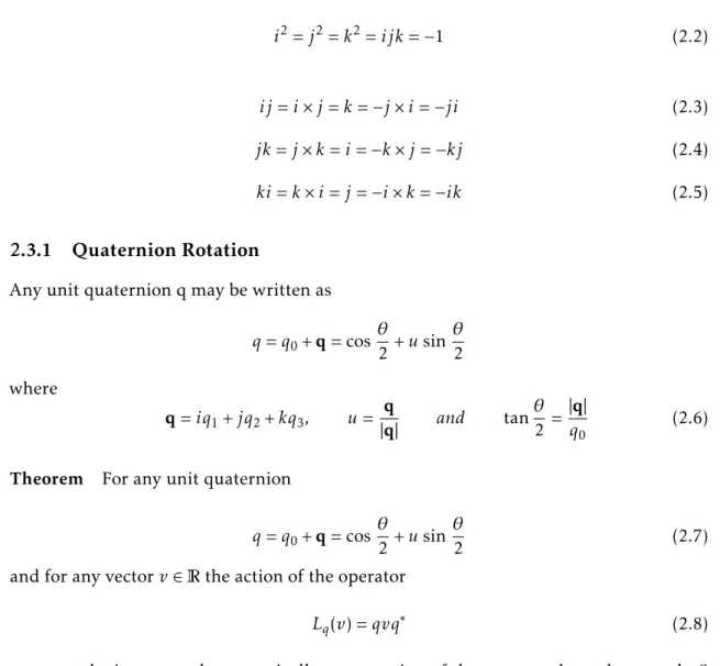
Any unit quaternion q may be written as
q = q0+ q = cos θ 2+ u sin θ 2 where q= iq1+ jq2+ kq3, u = q |q| and tan θ 2 = |q| q0 (2.6)
Theorem For any unit quaternion
q = q0+ q = cos
θ
2+ u sin
θ
2 (2.7)
and for any vector v ∈ R the action of the operator
Lq(v) = qvq
∗
(2.8) on v may be interpreted geometrically as a rotation of the vector v through an angle θ about q axis of rotation [31]. In Figure 2.3, we can see a representation of this rotation.
Figure 2.3: Quaternion rotation of vector v through an angle θ around the q axis of rotation, resulting in vector w. Adapted from [31].
2.4
Sensor Fusion
Sensor Fusion is the process of combining the information captured from multiple sensors in order to increase the accuracy of the measurement. In the case of the smartphone sensors, the information from the accelerometer, gyroscope and magnetometer is often used to rotate the reference frame of the measurements to one more adequate to the interpretation and processing of data, thus resulting in better data for analysis and use in many applications.
2.4.1 Complementary Filter
Complementary filters are applied to the smartphones IMU to compensate for the ac-celerometer’s high frequency noise and the gyroscopes low frequency drift in attitude estimation. They are also capable of dealing with artefacts resultant from magnetic inter-ferences. The complementary filter acts both as a low pass filter for the accelerometers data and a high pass filter for the gyroscopes data [32]. The filter can be formally repre-sented as
qt= α ∗ (qt−1+ qgyr) + (1 − α) ∗ qacc+mag (2.9)
q → quaternion representing the heading angle in degrees with respect to the
refer-ence frame
qgyr→quaternion representing the contibution of the gyroscope for the final heading angle
qacc+mag→quaternion representing the contribution of the accelerometer am magne-tometer to the final heading angle
α =τ+dtτ →time-related constant which defines the boundary between the contribu-tions of the accelerometer and the gyroscope signals. τ is time a constant which rep-resents how fast we want our filter to respond. dt is the period between acquisitions (samplingf requency1 )
In our situation, we want the filter to able to apply to all the possible step situations which can have a frequencies of up to 2Hz [19]. So a good value for α, with dt =100Hz1 and τ = 2Hz1 , will be
α = 0.5
0.5 +1001
≈0.98 (2.10)
The filter is also often used in the rotation of reference frames of the sensors in order to obtain more stable data.
2.4.2 Reference Frame
There are several reference frames applied to the analysis of the smartphones orientation and the acquisition of the sensors data. In some cases, a reference frame independent
2 . 4 . S E N S O R F U S I O N
of the smartphone position can provide an improvement in the stability of the collected data. This can be achieved through quaternion rotations and the data collected from the inertial sensors of the device.
2.4.2.1 Smartphone’s Reference Frame
The reference frame of the smartphone is the reference frame of the IMUs it contains. Usually, the reference frame of the smartphone is as the one represented in Figure 2.4 where the X axis points towards right of the smartphone, the Y axis towards top and the Z axis is pointing upwards, perpendicular to the smartphones screen.
Figure 2.4: Smartphone reference system. Retrieved from [11].
2.4.2.2 Earths Reference Frame
The Earth Reference frame is a reference frame where the z-axis is in the vertical direction, perpendicular to the earths surface and in an upwards direction, the y-axis is in the direction of the magnetic north pole and the x-axis is obtained through the outer product of the z and y axis vectors. This reference frame can be obtained using the accelerometer data to define the vertical direction,i. e. the Z-axis and the magnetometer data to define
Figure 2.5: Earth coordinates reference system.
2.4.2.3 User Reference Frame
The user Reference Frame is a reference frame where the the z-axis is in the vertical direction, pointing from the centre of the earth, the y-axis is in the direction the user is facing and the x-axis is obtained with the outer product of the z and y axis. The Z-axis can be estimated using the accelerometer data and the y-axis is obtained using a heading algorithm.
2 . 5 . M AC H I N E L E A R N I N G
2.5
Machine Learning
Machine learning (ML) can be described as a set of methods that can automatically detect patterns in data, and then use the uncovered patterns to predict future data, or to perform other kinds of decision making under uncertainty [33]. ML has seen vast application in
many fields of study and through time, a wide number of methods which have the ability to learn these patterns have emerged in many forms, varying in the type of action they perform and the way they learn. The learning process can occur in various manners and we can divide machine learning algorithms according to that.
2.5.1 Supervised Learning
In Supervised Learning we find algorithms which learn through the comparison of the output given by the ML algorithm and the target output,i. e. the algorithm is given a
set of input and target output (x, y) and it learns through an error estimate calculated with the difference between the estimated output ( ˆy) and the target output (y). Amongst Supervised Learning methods, we find Artificial Neural Networks, Decision Trees and Support Vector Machines.
2.5.2 Semi-supervised Learning
Semi-supervised learning (SSL) is a learning method between supervised and unsuper-vised methods. In some cases, the labelling of large data sets can be unfeasible due to the high amount of time and resources necessary. In these situations SSL can be of great use. In SSL algorithms a small amount of labeled data is mixed with the rest of the unlabeled data. This mixture assists the learning procedure greatly, which will result in higher accuracy results.
2.5.3 Unsupervised Learning
In Unsupervised Learning, the ML algorithms analyse the data and learn patterns ac-cording to the characteristics of data and not through reference values or targets. In Unsupervised Learning we find Hidden Markov Models, k-Means Clustering and Gaus-sian Mixture Models.
2.5.4 Reinforcement Learning
In Reinforcement Learning, an agent (e.g. a bot) tries to learn the sequence of actions
which will result in the highest cumulative reward. The concept of reward is similar to the reward given to dogs when trying to teach them a command, you give them a treat every time they respond correctly to the command and in time they will respond correctly more often, resulting in a higher cumulative reward.
2.5.5 Evaluation Metrics
The evaluation of the results can be made through several metrics. In the case of a binary classification problem, and using our case as an example, we classify each result, in comparison with the ground truth data, as:
• True Positive - a step is correctly identified where there is a step • False Positive - a step is incorrectly identified where there is no step • True Negative - a step is not identified where a step was not taken • False Negative - a step is not identified where one occurs
Accuracy It is a metric which measures the percentage of correct classifications (True Positives + True Negatives) that occurred. Accuracy, can be formally represented as
Accuracy =T rue P ositives + T rue N egatives
All T est Data (2.11)
Recall It’s a percentage of correct classification (T rue P ositives) which occured among all which should result in positive classifications (T rue P ositives + False N egatives) and is formally represented as
Recall = T rue P ositive
T rue P ositive + False N egative (2.12)
Specificity It’s the rate of correct negative classifications, i.e. the True Negative Rate,
and can be formally represented as
Specif icity = T rue N egative
T rue N egative + False P ositive (2.13)
Precision It’s the rate of True Positives among all positive results. Precision is formally represented as
P recision = T rue P ositive
T rue P ositive + False P ositive (2.14)
F-score In the evaluation of a classifiers performance, a score can be used. This F-score is the combination of precision and recall and can be formally represented as
F − score = 1 2
Recall +
1
P recision
2 . 6 . A R T I F I C I A L N E U R A L N E T WO R K S
2.5.6 Data Sets
In order to attain the best generalization from machine learning algorithms it is important to evaluate how the algorithm should learn from the data. Taking this into account, separation of the data into at least two different data sets, the training and testing data sets, is needed. This separation is important in order for the machine learning algorithm to learn properly from the provided information and to analyse how it deals with new information it has not seen before after the training procedure. It is important that these two data sets do not contain data in common in order to prevent issues such as overfitting. One further group of data can be employed, the validation data set, which is used in order to analyse the learning procedure into further detail.
Training Data Set The training data set is the group of data the model is going to use to learn from. This data set usually amounts for the highest percentage of the data in order to give the model to opportunity to learn as much as possible.
Validation Data Set The validation data set is used to analyse the training procedure of the model. This data set amounts for a small percentage of the training data, which is removed from the training data set. Through the analysis of the metrics from the validation data set throughout the training procedure, we can withdraw conclusions about the training of the model such as if it is overfitting, if some parameters need to be adjusted or even analyse what the best amount of training time for the model is.
Testing Data Set This data set is used to test the model after training. This data set has data that the machine learning model has not seen yet and through the testing data we can analyse if the resulting model can generalize well or if some adjustment is needed.
2.6
Artificial Neural Networks
Artificial Neural Networks (ANNs) are a type of machine learning algorithm based on the functioning of the biological neural networks. In the human brain, a neuron receives information from other neurons. That information is then processed and sent to next neuron, and this happens until the information reaches its target. ANNs are a simplified version of the biological neural networks.
ANNs use layers of neurons. Inside each neuron, the N inputs (xi) are processed and summed through linear combination with the neurons weight (w) and a bias (bias) parameters. Then, this value goes through an activation function (σ ) which gives us the output of the neuron. One common activation function is the sigmoid function [34].
a =
N X
i=0
σ (a) = 1
1 + e−a (2.17)
2.6.1 Activation Functions
Activation functions, as the name suggests, activate the neuron depending on the input values. These functions dictate the level of activity of the neuron through threshold values which, in term, will result in its output value. Several activation functions have been proposed through time in order to adapt neural networks to new challenges and applications and to improve its processing speed.
2.6.1.1 Linear
A linear activation function picks up the input multiplied by the weight and the added bias values and outputs a value proportional to it. This activation function allows for multiple output values which are linearly proportional to the input.
σ (a) = constant ∗ a (2.18)
Figure 2.7: Linear activation function
2.6.1.2 Sigmoid or Logistic function
The sigmoid or logistic function is mathematically described by
σ = 1
1 + e−a (2.19)
This function has output values in the interval [0, 1] and for that reason has seen multiple applications in fields of study where a probabilistic output of the neural network is needed [35].
2 . 6 . A R T I F I C I A L N E U R A L N E T WO R K S
Figure 2.8: Sigmoid activation function
2.6.1.3 Rectified Linear Unit (ReLU)
The Rectified Linear Unit or ReLU, is an activation function which only activates with positive input values and exhibits a linear behaviour. Its commonly used in convolutional neural networks due to allowing faster convergence speeds, helping to prevent exploding or vanishing gradients and for its computational efficiency [36].
σ (a) = a, if a ≥ 0 0, if a < 0 (2.20)
Figure 2.9: Rectified Linear Unit (ReLU)
2.6.1.4 Softmax
Softmax is an activation function used to give a probabilistic output in multiple class classification problems. This activation function is applied in the next to last layer of the network in order to transform the non-normalized output of the neurons into a probabil-ity value and the sum of the resulting probabilities assigned to each class are equal to 1. This activation function is applied in classification problems with 3 or more classes [34].
pi=
eai
PNk
k=0eak
ai→input label for the label used to calculate the loss
N → Number of input values pi→Predicted probability value
2.6.2 Loss/Cost Function
In this work we will define loss functions as a mathematical expression used to give a scalar value to the error between the desired output and the estimated one of the training data of the network in 1 epoch.
These functions play a very important role in the learning process of neural networks, since the gradients of the loss functions are used in backpropagation to adjust the param-eters of the network.
2.6.2.1 Mean Squared Error (MSE)
This loss function is frequently used in regression problems using neural networks.
Mean Squared Error = 1
N
N X
i=0
( ˆyi−ti)2 (2.22)
N → Size of training data ti→Target output
ˆ
yi→Predicted output 2.6.2.2 Cross-Entropy
Cross-entropy loss function is used in classification models where the output is expected to be binary.
Binary Classification In the cases where we have a binary classification problem,i. e.
we only have two classes as possible outputs,e. g. dog/not dog, the cross-entropy loss can
be calculated as
Loss = −(t · log( ˆy) + (1 − t) · log(1 − ˆy)) (2.23)
t → Target output
ˆ
y → Predicted output
Multiple Classes When we have 3 or more classes, loss in given by the sum of the loss values of each individual class
Loss = − N X i=0 t · log( ˆy) (2.24) N → Number of classes
2 . 6 . A R T I F I C I A L N E U R A L N E T WO R K S
t → Target output for the class
ˆ
y → Predicted output
2.6.3 Backpropagation
In order for the network to learn, an adjustment of the neurons parameters has to be made in an amount proportional to the loss. This is done through backpropagation of errors through the network. The calculation of the change needed to the parameters starts in last layer (output layer) and works backwards in order to compute how they should alter in order to improve the performance of the network,i.e. minimize the loss function.
We retrieve information about the changes the network needs to receive through the gradient of the loss function. We know that loss, assuming we are using equation 2.22, is
Loss = 1 N N X i=0 ( ˆyi−ti)2 (2.25)
and that the output value of our network are given by ˆ
yi= σ (aL−1i ∗wLi + biasLi) (2.26) with σ representing the activation function, aL−1i representing the output of the previous neuron, wiL representing the weight assigned, biasLi representing the bias value of the neuron and with the superscript L representing the number of the layer of the neuron. The gradient of the loss will be given by
Loss = 1 N N X i=0 ∇( ˆyi−ti)2= 1 N N X i=0 ∂Loss ∂ ˆyi (2.27) This gradient of the loss tells us the direction of highest increase of the loss function. We’re are looking to minimize it so we need the negative value of the gradient. This minimization of the loss function is called Gradient Descent.
To figure out how the parameters of the network affect the gradient, i.e. the partial derivatives of the Loss with respect to each weight and bias of the network, we start by analysing the output layer. In order to simplify the explanation, we will consider a ANN with only one neuron in each layer and we will represent the linear combination of the input of the neuron with the parameters (aL−1∗wL+ biasL) as zLresulting in
ˆ
y = σ (zL) (2.28)
We want to know the impact that changing the weights of the neuron will make to the loss function and in which direction. We know changing the weight will cause a change in the value of the function zL. That change can be represented by
∂zL ∂wL = a
This shift in zLwill then cause a shift in the value of our output ˆy which can be represented as ∂ ˆy ∂zL = σ 0 (zL) (2.30)
and as a consequence, this shift in the output ˆy will cause a change in the loss value which
can be expressed as
∂Loss
∂ ˆy = 2 ∗ ( ˆy − t) (2.31)
Through thechain rule, we can then express the derivative of the loss function with respect
to the weight as ∂Loss ∂wL = ∂zL ∂wL ∂ ˆy ∂zL ∂Loss ∂ ˆy (2.32)
The partial derivative of the Loss function in respect with the weight of the neuron will be
∂Loss
∂wL = a
L−1σ0
(zL)2 ∗ ( ˆy − t) (2.33)
The chain rule is applicable to the calculation of the partial derivatives of the loss of the rest of the network. In the case of a neuron in the second to last layer, the change in the weight of the neuron would change the value of zL−1 represented by
∂zL−1
∂wL−1 (2.34)
the change in zL−1would shift aL−1in the manner
∂ ˆaL−1
∂zL−1 (2.35)
the shift in the output of the neuron will change the value of z of the following neuron in the manner
∂ ˆzL
∂aL−1 (2.36)
and these changes will influence the loss value through the chain rule, resulting in
∂Loss ∂wL−1 = ∂zL−1 ∂wL−1 ∂ ˆaL−1 ∂zL−1 ∂ ˆzL ∂aL−1 ∂ ˆy ∂zL ∂Loss ∂ ˆy (2.37)
To study the influence of neurons in subsequent layers, we just need to follow the same procedure. This process allows us to obtain the partial derivatives we find in the gradient of the Loss function and as such, find the amount and direction of the adjustment the neurons need to improve performance.
For the realistic situation, where we have multiple neurons in each layer, lets use the network in figure 2.10 as an example. In this case, the neurons in the second to last layer
2 . 6 . A R T I F I C I A L N E U R A L N E T WO R K S
will influence loss through all the neurons in the subsequent layer, so we need to take this into account in the calculation of the derivative of the first weight of the neuron. This can be formally expressed by
Figure 2.10: The weight of the neuron will impact the loss value through all the neurons it is connected to. ∂Loss ∂wL−101 = ∂zL−11 ∂wL−101 ∂ ˆaL−11 ∂z1L−1 ∂ ˆzL0 ∂aL−11 ∂ ˆy0 ∂zL0 ∂Loss ∂ ˆy0 + ∂z L−1 1 ∂wL−101 ∂ ˆaL−11 ∂zL−11 ∂ ˆzL1 ∂aL−11 ∂ ˆy1 ∂zL1 ∂Loss ∂ ˆy1 (2.38) which can be simplified as
∂Loss ∂w01L−1 = ∂zL−11 ∂wL−101 ∂ ˆaL−11 ∂zL−11 NL X i=0 ∂ ˆzLi ∂aL−11 ∂ ˆyi ∂zLi ∂Loss ∂ ˆyi (2.39) and the expressing inside the sum is the various contributions of the output of the neurons to the loss through the neurons in the subsequent layer, resulting in
∂Loss ∂w01L−1 = ∂zL−11 ∂wL−101 ∂ ˆaL−11 ∂zL−11 NL X i=0 ∂Loss ∂aL−11 (2.40)
This process can be applied to all neurons in the network.
2.6.3.1 Learning Rate
Learning rate is a parameter used to adjust how fast we want the network to learn, i.e. how fast we want to lower the loss value and adjust the weights and biases of the network. The learning rate parameter is applied at the moment of update of the weights and biases in the following manner
wt+1= wt−α
∂Losst
Learning Rate Decay When we are nearing the convergence, it’s more useful to start reducing the amount of the changes performed through backpropagation. This is possible through a reduction of the learning rate through time/epoch and is called learning rate decay. Learning rate decay will reduce the learning rate each epoch and allow for smaller and smaller adjustments as training progresses. It can be formally represented as
α = 1
1 + DecayRate ∗ epoch·α (2.42)
2.6.4 Network Optimization
The optimization functions are used in order to bring the neural network to a minimum value of loss in the most efficient manner possible. They act in the moment of the update of the parameters of the network in an attempt to optimize the process. Many optimiza-tion algorithms have been proposed through time trying to improve several aspects of the learning process of ANNs and for many applications.
2.6.4.1 AdaGrad
Adaptive Gradient algorithm or AdaGrad is an optimization algorithm proposed byDuchi et al. [37] which incorporates knowledge from previous iterations to improve the
opti-mization process. It’s mathematically represented by
wt+1= wt−α ∗ 1 pεI + diag(Gt) ·∂Losst ∂wt (2.43) α → learning rate ε → constant I → Identity matrix
Gt→sum of the outer products of the gradient until t
Losst→Loss at time t 2.6.4.2 RMSProp
RMSProp is an adaptive learning rate optimization method. It uses the moving average of the squared gradient of the weight in order to adaptively modify the learning rate. This dampens the oscillations of the loss function during optimization and allows for faster convergence. It is formally represented by
wt+1= wt− α p E[g2] t ∂Loss ∂wt (2.44) E[g2]t+1= βE[g2]t+ (1 − β)( ∂Loss ∂wt ) 2 (2.45)
E[g2] → moving average of squared gradients
2 . 6 . A R T I F I C I A L N E U R A L N E T WO R K S
w → weight
β → moving average constant
2.6.4.3 Adam - Adaptive Moment Estimation
Adam is a optimizer proposed by [38] and combines the strong point of both AdaGrad, which works well with sparse gradients, and RMSProp which works well on online and non-stationary settings. The algorithm is formally represented by
wt+1= wt−α · ˆ mt+ 1 √ ˆ vt+ 1 + ε (2.46) α → learning rate w → weight mt+1= β1·mt+ (1 − β1) · gt→momentum estimation vt+1= β2·vt+ (1 − β2) · g2
t →RMSProp momentum estimation
gt→gradient ˆ
mt+1=(1−βmt+1t+1
1 )
→momentum bias correction ˆ
vt+1= vt+1
(1−βt+1
2 )
→RMSProp momentum bias correction
β1→momentum moving average constant
β2→RMSProp moving average constant
2.6.5 Network Regularization
In order to prevent overfitting problems, regularization techniques emerged and are a very important part of the development of neural networks.
2.6.5.1 L2 and L1 Regularization
These regularization techniques place a penalty value in the calculation of the loss and prevent the network from making strong assumptions,i.e. prevents the networks weights
from reaching high values.
L2 Regularization In the case of the L2 regularization, also called Ridge Regularization, we have Loss = Loss + λ 2N X ||w||2 (2.47) λ → regularization parameter
||w||2→euclidean norm of the weight squared
N → number of parameters
This method reduces some parameters making them smaller, helping reduce the attempt to learn specific information such as noise.
L1 Regularization In case of the L1 regularization, also called Lasso Regularization, we have Loss = Loss + λ 2N X ||w|| (2.48) λ → regularization parameter
||w|| → euclidean norm of the weight squared
N → number of parameters
This method reduces some parameters to zero, and because of this characteristic, it is used in implementations where we’re looking to compress the neural network and make it more simple.
2.6.5.2 Dropout
Dropout is a regularization technique which randomly deactivates neurons temporarily from the network layers and their respective connections. Each neuron has a probability to drop, which can be defined by the user, and it is the same for all neurons in the neural network [39].
Figure 2.11: (a) Normal neural network. (b) Dropout regularization technique. Some neurons and their connections are temporarily removed. Retrieved from [39].
2.6.5.3 Early Stopping
Early stopping is a regularization method which stops the training of the network based on a criteria set by the user. Early stopping is used to stop the training whenever the validation loss stops decreasing. This shift in the rate of change of validation loss can rep-resent the beginning of overfitting of the network. The user can also define a number of consecutive epochs where the criteria for early stopping needs to be met before stopping the training of the network in order to guarantee the networks stops when the training has reached its maximum.
2 . 6 . A R T I F I C I A L N E U R A L N E T WO R K S
2.6.6 Types of ANNs
The simplest artificial neural networks are composed of three layers, an input layer, one hidden layer and one output layer. An ANN can have a infinite number of hidden layers and there are many variations of neural networks where the behaviour of the neurons is modified, the connection between layers and neurons is different and these and other modifications change the overall function and application of the ANN. We will present some of the most relevant implementations.
2.6.6.1 Fully Connected Neural Network
As the name suggests, in this neural network all the neurons in one layer are connected to all the neurons in the next layers. The neurons do not connect with the preceding layers or with neurons from the same layer, keeping the information moving forward. In this implementation, all the neurons in one layer will have an impact in the final output of all the neurons in the next layer.
Figure 2.12: Fully connected neural network representation. Retrieved from [35].
2.6.6.2 Recurrent Neural Networks
"Recurrence is defined as the process of a neuron influencing itself by any means or by any connection"[35]. Traditional Recurrent Neural Networks are able to have this recurrence
by feeding the previous output back to the new input. This allows RNNs to better learn temporal features and patterns of the data.
Figure 2.13: Recurrent Neural Network representation. Retrieved from [35].
2.6.6.3 Long Short Term Memory(LSTM) Neural Networks
LSTM Neural Networks were proposed by S. Hochreiter and J. Schmidhuber. [40] in order to solve exploding and vanishing gradient problems which common RNN faced during backpropagation. This was achieved through the implementation of memory cells and gates. The memory cells allow a longer term internal storage of previous data when compared to RNNs and the gates give the ability to control the flow of information, and select the data features to retain or dismiss in the calculation of the output. This neural network is able to receive and process sequences of data and learn long term dependencies.
2.6.6.4 Convolutional Neural Networks
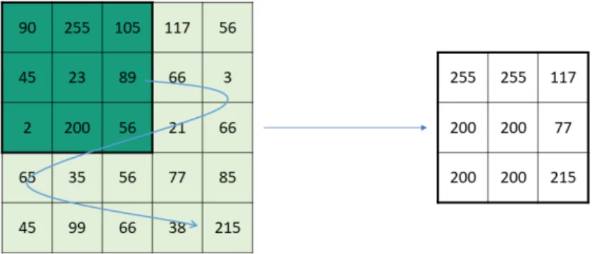
In applications of neural networks such as the recognition of handwritten digits and the analysis of images, there are spatial features which are important in order to achieve the desired output of the network. Convolutional neural networks (CNNs) are one of the best approaches for these application due to the way they analyse the image data. In the analysis of an image, the CNN applies convolution to the data through filter/kernels with dimension height per breath per number of channels and the input for the convolution are the values of the pixels captured by the kernel. These kernels move throughout the whole image.
Convolution Operation In the convolution operation, the filter "overlaps" the data and value of the data in each cell is multiplied by the value of filter in the same cell. This multiplication occurs in to all the value of the data to which the filter is being applied. The result of the individual multiplications are then summed to give the result of the convolution operation.
2 . 6 . A R T I F I C I A L N E U R A L N E T WO R K S
Figure 2.14: Convolution operation.
Both the size of the kernel and the steps/strides taken while moving through the image can be adjusted to improve results. This analysis of smaller parts of the image instead of the image as a whole allow for better analysis of important details and reduces the computational requirements. One important strength of CNNs is that in models with several CNNs, the first layers extract low levels features such as shapes and borders and subsequent layers extract higher level features such as faces or objects from an image.
Pooling Pooling operation is also a part of many convolutional neural network. This operation allows for the selection of the features of highest relevance resulting from the convolution operations and helps improve the computational efficiency of the network.
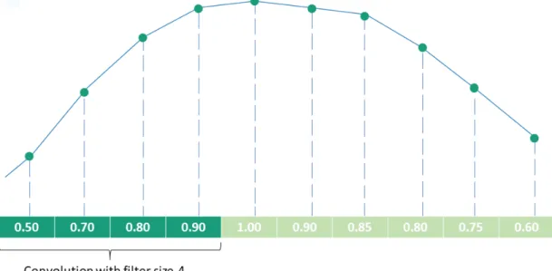
1 Dimensional Convolutional Neural Networks 1D Convolutional Neural Networks work in a similar fashion to traditional convolutional neural networks. Instead of apply-ing convolution to 2 or 3 dimensional data such as images, it applies 1 dimensional data which is the case of the smartphone’s accelerometer, gyroscope and magnetometer. The filter runs through the data, as exemplified in Figure 2.16, applying convolution. The filter can also run through the several axis of a sensor simultaneously.
Figure 2.16: 1D Convolution. The kernel with size 4 moves along the data and performs convolution.
C
h
a
p
t
e
r
3
Da ta Ac q u i s i t i o n
The goal of this thesis is to develop an algorithm capable of performing step detection with high accuracy in an unconstrained manner. For the training and testing of the algorithm, a data set which comprises of several of different situations and movements a normal individual encounters in day to day activities is essential, and that was taken into account in the development of the acquisition protocol. Two different data sets were recorded, an indoor data set with a predefined course and set of actions and a free living data set.
3.1
Sensors Acquired
For data collection for both training and testing of the algorithm, the accelerometer, gyroscope and magnetometer data where recorded using a set of two Pandlet Recorders and a Nexus 5 smartphone.
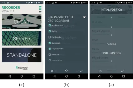
Fraunhofer AICOS Pandlets (Figure 3.1) are small sensing devices with several sensors incorporated, including a tri-axial IMU with an accelerometer, a gyroscope and a magne-tometer. Due to its small size, these devices are easily attached to and individual for data collection. The Pandlets also come with an embedded Bluetooth module, allowing the wireless connection with external devices. These devices allow the recording of inertial data at 100 Hz [41].
Figure 3.1: Fraunhofer AICOS Pandlet
Nexus 5 smartphone also comes with tri-axial accelerometer, gyroscope and magne-tometer sensors which record data with a 200 Hz sampling frequency[42].
The data was collected through a mobile application developed by Fraunhofer AICOS, the Recorder App. This app allows the collection of data from the smartphones many sensors and also from external sensors simultaneously, through a Bluetooth connection.
(a) (b) (c)
Figure 3.2: (3.2a) Fraunhofer AICOS Recorder App. (3.2b) Connection to Pandlets and sensor selection. (3.2c) Final acquisitions annotations screen.
3.2
Indoor Data Acquisition
Using the Pandlets and the Nexus 5 smartphone, several data acquisition sessions were conducted with multiple volunteers. For the Indoor Data Set a total of 7 volunteers and for the Free Living Data Set a total of 11 volunteers, with ages between 22 and 29 years old and without prior gait related disabilities, performed the acquisition protocols.
3 . 2 . I N D O O R DATA AC Q U I S I T I O N
3.2.1 Sensor Placement
The Pandlets were used to record data to obtain the Ground Truth of the steps while the smartphone recorded the users movement in several positions and movement speeds found in the day to day routine. The Pandlets were placed over the volunteer’s ankles in order to obtain the best signal possible for step detection. This Pandlet placement allows for the detection of clear peaks from the accelerometer signal and also for the clear detection of the cyclical nature of the swing and stance phases of gait through the gyroscope.
The smartphone placements were:
• Texting - smartphone held in front of the upper abdomen/lower chest area in a texting position
• Calling - smartphone held close to one of the ears of the user similarly to when answering a phone call
• Handheld - smartphone held in one of the hands with arm straight and beside the trunk
• Jacket Front Pocket - smartphone stored in one of the front pockets of the jacket • Front Pocket - smartphone placed in one of front pocket of jeans
• Back Pocket - smartphone placed in the back pocket of jeans
3.2.2 Recorded Activities
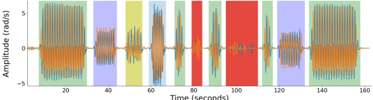
In the selection process of the movements to analyse using the inertial sensors of the smart-phone and Pandlets, both step related movements and false step/false positive related movements were taken into account for the protocol. The final list of user movements analysed were:
• Walking - walking in a natural pace
• Running - running in a natural/jogging pace
• Walking while dragging feet - walking while purposely dragging the feet on the floor to recreate the walking of people with some gait impairment or the walking of elderly individuals
• Walking downstairs - normal pace walking downstairs • Walking upstairs - normal pace walking upstairs
• Jumping - jumping without moving from the current position. The purpose of the movement is to prevent the detection as step. Jumps have high inertial signal amplitude and as a consequence can be easily misdetected as steps.
![Figure 2.1: Gait cycle temporal division. Retrieved from [29]](https://thumb-eu.123doks.com/thumbv2/123dok_br/15617361.1054484/30.892.164.767.913.1121/figure-gait-cycle-temporal-division-retrieved.webp)
![Figure 2.2: Gait cycle Rancho classification. Retrieved from [29]](https://thumb-eu.123doks.com/thumbv2/123dok_br/15617361.1054484/32.892.249.684.141.583/figure-gait-cycle-rancho-classification-retrieved.webp)
![Figure 2.12: Fully connected neural network representation. Retrieved from [35].](https://thumb-eu.123doks.com/thumbv2/123dok_br/15617361.1054484/49.892.262.598.532.792/figure-fully-connected-neural-network-representation-retrieved.webp)