water
ArticleMonthly Prediction of Drought Classes Using
Log-Linear Models under the Influence of NAO for
Early-Warning of Drought and Water Management
Elsa Moreira1,* ID, Ana Russo2 ID and Ricardo M. Trigo2
1 Center of Mathematics and Applications (CMA), Faculty of Sciences and Technology, New University of Lisbon, 2829-516 Caparica, Portugal
2 Instituto Dom Luiz (IDL), Faculty of Sciences, University of Lisbon, 1749-016 Lisboa, Portugal; acrusso@fc.ul.pt (A.R.); rmtrigo@fc.ul.pt (R.M.T.)
* Correspondence: efnm@fct.unl.pt
Received: 3 November 2017; Accepted: 10 January 2018; Published: 12 January 2018
Abstract:Drought class transitions over a sector of Eastern Europe were modeled using log-linear models. These drought class transitions were computed from time series of two widely used multiscale drought indices, the Standardized Preipitation Evapotranspiration Index (SPEI) and the Standardized Precipitation Index (SPI), with temporal scales of 6 and 12 months for 15 points selected from a grid over the Prut basin in Romania over a period of 112 years (1902–2014). The modeling also took into account the impact of North Atlantic Oscillation (NAO), exploring the potential influence of this large-scale atmospheric driver on the climate of the Prut region. To assess the probability of transition among different drought classes we computed their odds and the corresponding confidence intervals. To evaluate the predictive capabilities of the modeling, skill scores were computed and used for comparison against benchmark models, namely using persistence forecasts or modeling without the influence of the NAO index. The main results indicate that the log-linear modeling performs consistently better than the persistence forecast, and the highest improvements obtained in the skill scores with the introduction of the NAO predictor in the modeling are obtained when modeling the extended winter months of the SPEI6 and SPI12. The improvements are however not impressive, ranging between 4.7 and 6.8 for the SPEI6 and between 4.1 and 10.1 for the SPI12, in terms of the Heidke skill score.
Keywords: drought classes; Standardized Precipitation and Evapotranspiration Index (SPEI); Standardized Precipitation Index (SPI); North Atlantic Oscillation (NAO); log-linear modeling; persistence
1. Introduction
The social, environmental and economic impacts of drought, as well as its features, have been studied in numerous studies [1–7]. Since 1950, a positive tendency of drought patterns has been observed over some regions of the globe [8–10], in part due to global warming [11]. Within the European context, the positive drought trends seem to be particularly acute in the Mediterranean area [10,12,13], where increased dryness [14–16] and temperature is more notorious [6,17]. As shown in a recent study by Dumitrescu et al. [18] covering all of Romania over the period 1961–2013, the most striking results concern the number of summer days, which has increased by 95% in of the considered stations, while an increase in the duration of warm spells of 83% has been observed in the same stations. In a paper by Spinoni et al. [19], the drought events in the last five decades in the Carpathian region (ranging from the Czech Republic to Serbia, encompassing Slovakia, Poland, Hungary, Ukraine, and Romania) were analyzed. The most intense droughts took place in 1990, 2000, and 2003, followed
Water 2018, 10, 65 2 of 24
by other 10 notable events. In general, for that region, the drought frequency is slightly increasing, however, the rise has not been confirmed by significance tests [19].
Under the current global warming process [17], in the next decades an increase in the frequency, duration, and affected area of drought events in the drought-prone areas like the Mediterranean is expected [11,16,20–22]. The Carpathian region shows a dual behavior, as in the past it was reported as being generally affected by increasingly frequent and severe droughts [19] and, according to future drought projections, more extreme changes are expected in the Carpathian Mountains than in the surrounding regions. Besides the regional differences, seasonal differences are also expected, with more frequent droughts in spring and summer and a stronger decrease of winter droughts [23]. Changes in the agriculture forest sector in Romania have been shown to be directly affected by the weather and climatic conditions [24,25], as recognized within the Romanian National Climate Change Strategy (2013–2020), in its adaptation component [26]. In particular, drought is a major cause of unexpected crop failure [27–29]. Future changes of climatic conditions in Romania will drive additional changes in crop production in the region [24,25,30] and the sector is expected to continue to be affected in the future [30,31]. Therefore, for countries and stakeholders considering the implementation of appropriate preparedness and mitigation measures, it becomes increasingly important to develop robust early warning systems [3,32]. However, under the current state of the art, it is extremely challenging to forecast the early stages of a drought, as well as its expected conclusion, particularly in the middle latitudes [33]. Nevertheless, considering that droughts evolve slowly, it is increasingly feasible to release a timely prediction allowing for some measures to be adopted to mitigate the effects of the drought [32,34,35]. In this context, drought predictions at a monthly scale can be beneficial so that resource managers and water users can prepare for the occurrence of various stages of a drought, including onset, duration, or conclusion.
The assessment of drought severity can be achieved with a number of indices developed for that purpose, such as the Palmer Drought Severity Index (PDSI) [36], and the MedPDSI [37,38], etc. In recent years, it has been shown that the use of multi-scalar drought indices is quite useful, including the Standardized Precipitation Index (SPI) [39] and the Standardized Precipitation Evapotranspiration Index (SPEI) [40]. In this study, the SPI and SPEI were the chosen indices because of their multi-scalar nature that allows assessing drought impacts, for different time scales, on soil moisture, snowpack, reservoir storage, groundwater, and stream-flow [39,40]. Although droughts are mostly controlled by the temporal variability of precipitation, in a context of global warming, the temperature variable may play an increasing role in drought assessments, and therefore the SPEI was also considered. Thus, while the SPI is computed only based on precipitation, the SPEI is sensitive to changes in the evaporation demand (caused by temperature fluctuations and trends) because it considers the effect of potential evapotranspiration (PET) on drought severity [10,40].
On the other hand, atmospheric circulation plays a major role in terms of precipitation occurrence but also on its frequent inhibition of precipitation leading to drought on different time and spatial scales (e.g., [41,42]). The main features of the atmospheric circulation for the European region are captured by a set of large-scale patterns (and corresponding indices) that are usually computed at the monthly/seasonal temporal scales [43]: the North Atlantic Oscillation (NAO), the East-Atlantic (EA) pattern, the Scandinavian (SCAND) pattern, and the East-Atlantic Western Russia (EAWR) pattern. The temporal indices associated to these patterns are freely available at the National Centers for Environmental Prediction (NCEP) website. It is now well established that the main pattern controlling wet and dry rainfall regimes over Western Europe is the NAO mode [44–46]. However, this effect extends to the eastern part of the Mediterranean. In fact, when the NAO is in its positive phase (i.e., NAO+), winter storms coming from the Atlantic are deflected northward, resulting in wet winters over the northern part of Europe, dry winters over the southern and eastern part of Europe [47,48], and also lower-than-average temperatures [45]. Thus, the NAO+ regime is associated to below-average precipitation over most southern and central European regions and higher-than average values in Northern Europe [45–48]. In contrast, when the NAO is in its negative phase (i.e., NAO−) storm
tracks are shifted southwards, promoting wet and mild winters over the southern and eastern parts of Europe and dry winters over the northern part of Europe [45–48].
The region focused on this study is the Prut River basin in Eastern Europe (Figure1). The Prut River source is located in the Carpathian Mountains, Ukraine, and runs into the Danube River. It is circa 1000 km long, and its catchment area is 27,540 km2. The basin of the Prut River, being a transboundary basin, is located in the territory of three countries: 28% in Moldova; 33% in Ukraine; and 39% in Romania (Figure1). The Romanian territory is divided by the Carpathian Mountains into two groups of regions: the intra-Carpathian regions and extra-Carpathian regions. The extra-Carpathian regions cover the southern, eastern, and southeastern parts of Romania, while areas located inside the mountain chain and those located westward from the mountains are considered the intra-Carpathian regions (Figure1). The Carpathian Mountains form an orographic border which imposes a separation between the regions influenced by mild oceanic (south and west) and continental (north and east) climates. In the last 20 years, a shift from oceanic to continental climate can be seen, especially in the Romanian part of the Carpathians [19]. The extra-Carpathian regions (delimited area in Figure1), which include most of the Prut basin, are more often influenced by southern tropical or eastern continental air masses [49]. The maximum flow of the Prut River is recorded during the beginning of the warm season, often in early April due to the significant quantities of precipitation overlapping with snowmelt, and manifests itself as spring–summer floods [50]. Although the Prut watershed has a relatively low water stress under present climate, a more detailed assessment is needed of this basin since its watershed has been exposed to landscape changes that may increase the runoff and reduce reservoir capacity [51]. Corduneanu et al. [50] studied the Prut river flow recordings during the period 1978–2012 and noticed that two extremely severe droughts occurred, one spanning from 1982 to 1988 and more recently another that began in 2011 and continued until the end of 2012. In addition, Croitoru et al. [49] studied the spatiotemporal distribution of aridity indices based on temperature and precipitation in the extra-Carpathian region of Romania and found that the southeastern region, including the Prut basin, are most vulnerable to semi-aridity, especially during the warm period of the year.
1
Figure 1. Map of Romania indicating the 15 grid points (from the Climatic Research Unit (CRU) database) covering the study area (delimited by a red line) and showing the Carpathians Mountains as well as the extra-Carpathian region [45] delimited here by a yellow line.
Water 2018, 10, 65 4 of 24
In terms of the influence of climate variability, Tomozeiu et al. [52] found a significant association between Romania’s precipitation variability in the winter months and large-scale circulation patterns, such as the NAO and the blocking phenomenon in the Atlantic-European sector. Bojariu and Giorgi [5] observed fine-scale features of the NAO precipitation signal over the Iberian, Scandinavian, Alpine, Balkan, and Carpathian regions, demonstrating the important role played by the topographic forcing in modulating the large-scale NAO variability over Europe. Additionally, a decreasing trend in winter precipitation was discovered, especially in the extra-Carpathian region, during the last two decades of the 20th century, likely related with an intensification of the NAO+ and a decrease in the frequency of blocking especially after 1980. The winter NAO signal was found by other authors to be stronger in the extra-Carpathian regions, as result of the orographic force on the atmospheric flow in the Carpathian Mountains [53]. Moreover, regions in Central and Eastern Europe were identified as having a source of NAO-related predictability [53], which results from the positive correlation present in the month of November between the thermal anomalies and the NAO index. This source of predictability might be used to predict the onset of the NAO in the following winter [53].
Several approaches to the have been proposed for the forecasting of droughts on a monthly basis, namely statistical, physical-based techniques, or hybrid techniques. Examples of those hybrid approaches which conjugate statistics and physical-based techniques are the works by Mishra et al. [54] and Kim and Valdes [55], which use respectively a hybrid stochastic and neural network model and the later conjugates wavelet transforms and neural networks for a nonlinear model. However, other examples are the model combination of the wavelet and fuzzy logic models used in Ozger et al. [56] and the adaptive neuro-fuzzy inference used in Bacanli et al. [57]. Among the techniques used for drought forecasting, statistical models are chosen many times, since they are simple to implement, do not have a high computational burden, and produce useful predictions [58]. There are a variety of statistical methodologies available which can be applied for the intended purpose, namely autoregressive integrated moving average (ARIMA)-type approaches [59,60], artificial neural network (ANN) models [61,62] or even other types of stochastic and probability models, such as Markov chains [63], log-linear models [64,65], and others [66,67]. A thorough discussion on various methodologies used for drought modeling and prediction showing the limitations and advantages of each modeling/technique was done by Mishra and Singh [58].
One approach often used to include useful information related to climate dynamics in drought forecasting models considers (as covariates) atmospheric–oceanic monthly or seasonal anomaly indices. Some examples of this type of approach include the use of ANN models and time series of drought indices, including the NAO index as a covariate [68], or the use of probabilistic models resulting from evaluating conditional probabilities of future SPI classes based on current SPI and NAO classes [67].
The combined effects of the NAO index and SPI time series’ information have been well explored in the context of Portuguese drought predictability, specifically to predict drought class transitions some months in advance based on the SPI of the previous months [57,58,62]. These models, which are three-dimensional log-linear, rely exclusively on probabilities of transition between states and are fitted to drought class transitions counts separately for the NAO+ and NAO−phases. Taking into account the NAO state in the current month, the most probable drought class transition for the next month and their confidence intervals are computed. This approach has proved its usefulness in predicting the SPI drought class one or two months in advance [64,65,69].
Considering the challenges in climate change, and the reported NAO influence on precipitation and, consequently, on drought occurrence in Romania and the Prut basin, the aim of this work is to assess the predictability of drought at a monthly scale for the Prut basin, with the objective of providing drought warnings for agricultural management. For this purpose, the same log-linear models are used fitted to drought indicators, the SPI, and for the first time also to SPEI class transitions, under the influence of the NAO index.
Additionally, we aim to go a step further from previous studies using log-linear models [64,65,69], identifying the predictors that can better predict changes of drought classes one or two months in
advance, namely with the use of a four-month NAO average as a predictor instead of the single lagged NAO value as in a previous study [65]. An analysis of the extended winter months (November–May) and the complete annual period was performed, as well a study of the use of different SPI (SPEI) drought class intervals, aiming at a better assessment of the Prut basin climate. Finally, with the aim of improving the study, the frequency of severe and extreme droughts and also wet events in three periods with similar numbers of years were statistically compared using an analysis of variance technique. 2. Data and Methods
2.1. Standardized Drought Indicators and the NAO
The climatic data used in this study were retrieved from the 0.5×0.5 gridded resolution CRU (Climatic Research Unit) time-series (TS) 3.23 produced by the Climatic Research Unit (CRU) at the University of East Anglia. The CRU TS 3.23 variables used for SPI and SPEI computation were monthly precipitation and mean temperature, for the period January 1901–December 2014, located over the Prut basin (Romania, Ukraine and Moldavia) (Figure1). Details regarding this dataset are available at the CRU high-resolution gridded database (https://crudata.uea.ac.uk/cru/data/hrg/).
The choice of the baseline period relative to which standardized drought indicators are calculated is a key factor [23]. If a shorter period (e.g., 30 years) characterized by frequent and severe droughts is used as a baseline, this may impinge influence on the indicator’s trend over the entire period [23]. This study focuses on class transitions over a long-term period, so we decided to use the entire period (1901–2014) as the baseline, thus ensuring more robust comparisons. Moreover, drought is different from other natural disasters and takes place when a significant deviation from the normal hydrologic conditions of an area occurs [36]. Thus, using as a baseline the past decades for estimating droughts over the years 1901–2014 might be problematic, as the last decades have shown an intensification of drought events relative to the beginning of the century, which might be unrealistic.
Moreover, the long-term period range, from 1901 to 2014, is considered an important pre-requisite since the log-linear modeling approach benefits from using long and recent data to better parameterize the models. Six- and twelve-month time-scales of both SPI and SPEI (SPI6, SPEI6, SPI12 and SPEI12) were computed from precipitation and temperature time series correspondent to the 15 grid points shown in Figure 1. The use of these two time-scales relies on the fact that each one reflects the accumulated drought conditions of longer or shorter periods. Specifically, the 12-month time scale is able to identify long-term dry and wet periods, being more representative of the impacts of drought on the hydrologic regimes [70]. In contrast, shorter time scales are useful to detect agricultural droughts [25], reflecting a better change of class instead of its persistence [70]. We would, however, like to highlight that the terms “short-term accumulation periods” and “long-term accumulation periods” in SPI/SPEI drought indicators here refer to meteorological droughts, as they use meteorological inputs and not, for example, soil moisture (agricultural drought), or low flow data (hydrological droughts).
For the SPI computation, the gamma distribution was used to model precipitation and for the SPEI, Penman–Monteith’s PET was used, as well as the log-logistic distribution to model the water deficit (D) [40].
The categories usually used to classify drought, and wetness classes are presented in Table1. However, to avoid problems in the model fitting [64] caused by too many class transitions with value zero, several classes were grouped. We have considered a total of four classes in our modeling analysis as in recent studies [65] albeit not necessarily exactly defined in the same way. Thus, a new unique wetness class grouping all the wetness categories was included, since our main focus in this study was drought prediction. The normal and the near-normal drought classes are grouped together, since, being near-normal, the first category of drought has low impacts, and therefore we do not find necessary to distinguish a single class for it. Lastly, both the severe and extreme drought classes are grouped due to the number of transitions attributable to the extremely severe drought classes, since
Water 2018, 10, 65 6 of 24
they occur considerably less frequently than the other classes. It must be noted that the number of classes and their arrangement in different works reflect, to a certain extent, the different frequency of these classes. Therefore, we are confident that the classification presented herein is more balanced for modeling purposes and may respond better to the climate features of the Prut basin.
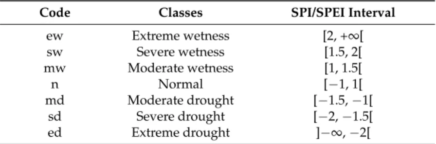
Table 1. Drought and wetness classes of the Standardized Precipitation Index/Standardized Precipitation Evapotranspiration Index (Adopted from Mckee et al. [39]).
Code Classes SPI/SPEI Interval
ew Extreme wetness [2, +∞[ sw Severe wetness [1.5, 2[ mw Moderate wetness [1, 1.5[ n Normal [−1, 1[ md Moderate drought [−1.5,−1[ sd Severe drought [−2,−1.5[ ed Extreme drought ]−∞,−2[
The monthly drought classes’ time series were categorized considering the limits defined in Table2reflecting the modifications described before, relative to both SPI and SPEI time series with 6-and 12-month time scales.
Table 2. Drought and wetness classes of SPI/SPEI for modeling purposes (modified from Mckee et al. [39]).
Code Classes SPI/SPEI Interval
1 Wet [1, +∞[
2 Normal/Near-Normal [−1, 1[
3 Moderate [−1.5,−1[
4 Severe/Extreme ]−∞,−1.5[
To cover the full period of available precipitation data (1901–2014), an extended historical record (starting in 1864) of a station-based NAO was computed for this study. This long NAO dataset relies upon the difference of normalized Sea Level Pressure (SLP) between Lisbon (Portugal) and Reykjavik (Iceland) and overcomes the problem of the available National Centers for Environmental Prediction (NCEP) Climate Prediction Center monthly NAO, which only dates back to 1950.
2.2. Correlations between SPEI/SPI and NAO
As a preliminary step, a simple correlation analysis was performed to evaluate the association between the SPEI (SPI) and the NAO index monthly time series for each time scale and grid point (Table3). The correlations with other large-scale indices like the EAWR and EA patterns influencing Central and Eastern Europe were also tested, and the highest correlations were always obtained with the NAO. Besides that, different NAO averages and lags with the SPI/SPEI were tested. For SPEI6/SPI6, the maximum inverse correlation was obtained with the NAO index average of the last four months, i.e., the NAO value at month t considered for the modeling is the simple four-month average ((NAO_(t−3) + NAO_(t−2) + NAO_(t−1) + NAO_t)/4). If that NAO > 0, then the NAO state is assigned positive (NAO+), otherwise it is considered negative (NAO−). For the SPEI12/SPI12, the maximum inverse correlation is obtained also with the last four-month average but with a lag of 1 month, i.e., with (NAO_ (t−4) + NAO_(t−3) + NAO_(t−2) + NAO_(t−1))/4. This correlation between the SPEI/SPI and the NAO was computed twice considering initially all the months of the year and afterward only the winter and spring months from November to May, commonly called the extended winter months. The analysis for the extended winter months was performed taking into account that the impact of the NAO pattern in Southern Europe is usually
better defined in this time of the year. The inverse correlation between the SPEI (SPI) and the NAO considering all the months of the year is, on average, lower by approximately 0.08.
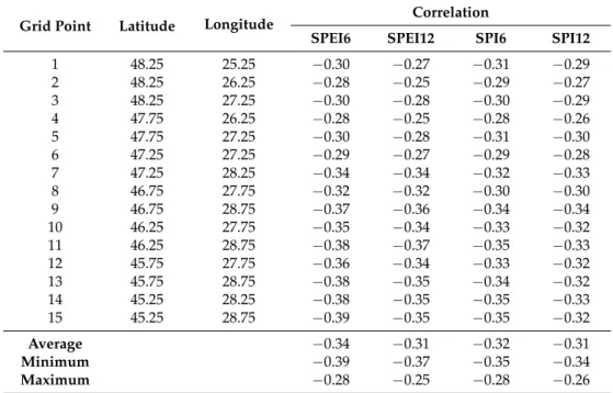
Table 3.Correlation between the SPEI (SPI) with 6- and 12-month time scales and the North Atlantic Oscillation (NAO) average of the last 4 months, considering only the extended winter months (November–May). The highest inverse correlation values are highlighted in bold.
Grid Point Latitude Longitude Correlation
SPEI6 SPEI12 SPI6 SPI12
1 48.25 25.25 −0.30 −0.27 −0.31 −0.29 2 48.25 26.25 −0.28 −0.25 −0.29 −0.27 3 48.25 27.25 −0.30 −0.28 −0.30 −0.29 4 47.75 26.25 −0.28 −0.25 −0.28 −0.26 5 47.75 27.25 −0.30 −0.28 −0.31 −0.30 6 47.25 27.25 −0.29 −0.27 −0.29 −0.28 7 47.25 28.25 −0.34 −0.34 −0.32 −0.33 8 46.75 27.75 −0.32 −0.32 −0.30 −0.30 9 46.75 28.75 −0.37 −0.36 −0.34 −0.34 10 46.25 27.75 −0.35 −0.34 −0.33 −0.32 11 46.25 28.75 −0.38 −0.37 −0.35 −0.33 12 45.75 27.75 −0.36 −0.34 −0.33 −0.32 13 45.75 28.75 −0.38 −0.35 −0.34 −0.32 14 45.25 28.25 −0.38 −0.35 −0.35 −0.33 15 45.25 28.75 −0.39 −0.35 −0.35 −0.32 Average −0.34 −0.31 −0.32 −0.31 Minimum −0.39 −0.37 −0.35 −0.34 Maximum −0.28 −0.25 −0.28 −0.26
As can be observed in Table3, the correlations values between NAO and SPEI (or SPI) in the Prut basin range in the interval [−0.39,−0.25], and the use of different drought indices does not provide added information, as no significant differences (for either time scale 6 or 12) can be observed between results attained with SPEI and SPI. Moreover, all the correlation values presented in Table3were found to be statistically different from zero at a 5% level.
2.3. Modeling
The number of two-step monthly transitions between drought classes was counted separately for NAO+ and NAO−, evaluated at the current month (t), to form two three-dimensional (4×4×4) contingency tables [65] with N = 64 cells each. The referred contingency NAO−and NAO+ tables present three categories and four levels each, respectively the drought class at months t−1, t, and t + 1, and drought classes 1, 2, 3, and 4, previously defined in Table2. Contingency tables for the SPEI6 and SPEI12 are presented in Tables4and5. On the other hand, SPI contingency tables, which are similar, are not shown for the sake of simplicity.
Log-linear modeling inputs correspond to the number of times that in each month the drought class i was followed by the drought class j in the following month and then by the drought class k in the month after that (two-step transitions) called the observed frequencies. The model computes the expected frequencies.
Modeling more than two step transitions with log-linear models is very difficult since we will get too many observed frequencies equal to zero, which brings fitting problems [71]. On the other hand, separately modeling the negative and positive phase of the NAO leads to simpler models, with fewer parameters and therefore easier adjustment.
Water 2018, 10, 65 8 of 24
Table 4.Counts of two consecutive transitions between drought classes of SPEI6 (t−1→t→t + 1) for NAO−and NAO+.
Water 2018, 10, 65 8 of 24
Table 4. Counts of two consecutive transitions between drought classes of SPEI6 (t − 1 → t → t + 1) for NAO− and NAO+.
NAO− Drought Class Month t + 1 Drought Class Month t + 1 Drought Class Month t + 1 Drought Class Month t + 1 1 2 3 4 Drought Class Month t – 1 Drought Class Month t Drought Class Month t Drought Class Month t Drought Class Month t 1 2 3 4 1 2 3 4 1 2 3 4 1 2 3 4 1 52 3 0 0 39 43 0 0 0 3 0 0 0 1 0 0 2 41 49 0 0 21 246 7 1 1 25 9 1 0 7 7 3 3 0 2 0 0 0 19 5 10 0 1 7 2 0 0 5 2 4 0 1 0 0 0 6 5 1 0 2 4 4 0 0 0 4 NAO+ Drought Class Month t + 1 Drought Class Month t + 1 Drought Class Month t + 1 Drought Class Month t + 1 1 2 3 4 Drought Class Month t – 1 Drought Class Month t Drought Class Month t Drought Class Month t Drought Class Month t 1 2 3 4 1 2 3 4 1 2 3 4 1 2 3 4 1 27 1 0 0 19 42 0 0 0 1 1 0 0 0 0 0 2 17 37 0 0 15 293 19 1 0 35 16 3 0 7 12 6 3 0 1 0 0 0 33 16 6 0 2 7 6 0 0 10 9 4 0 1 0 0 0 17 6 9 0 1 6 6 0 0 1 13
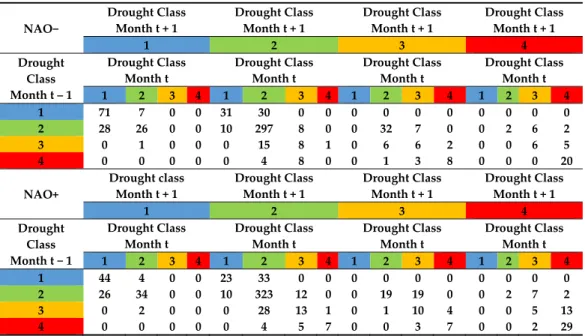
Table 5. Counts of two consecutive transitions between drought classes of SPEI12 (t − 1 → t → t + 1) for NAO− and NAO+.
NAO− Drought Class Month t + 1 Drought Class Month t + 1 Drought Class Month t + 1 Drought Class Month t + 1 1 2 3 4 Drought Class Month t – 1 Drought Class Month t Drought Class Month t Drought Class Month t Drought Class Month t 1 2 3 4 1 2 3 4 1 2 3 4 1 2 3 4 1 71 7 0 0 31 30 0 0 0 0 0 0 0 0 0 0 2 28 26 0 0 10 297 8 0 0 32 7 0 0 2 6 2 3 0 1 0 0 0 15 8 1 0 6 6 2 0 0 6 5 4 0 0 0 0 0 4 8 0 0 1 3 8 0 0 0 20 NAO+ Drought class Month t + 1 Drought Class Month t + 1 Drought Class Month t + 1 Drought Class Month t + 1 1 2 3 4 Drought Class Month t − 1 Drought Class Month t Drought Class Month t Drought Class Month t Drought Class Month t 1 2 3 4 1 2 3 4 1 2 3 4 1 2 3 4 1 44 4 0 0 23 33 0 0 0 0 0 0 0 0 0 0 2 26 34 0 0 10 323 12 0 0 19 19 0 0 2 7 2 3 0 2 0 0 0 28 13 1 0 1 10 4 0 0 5 13 4 0 0 0 0 0 4 5 7 0 0 3 7 0 0 2 29
Contingency Tables 4 and 5 show that the most frequent drought transitions correspond to a persistent condition which implies the maintenance of the previous drought classes, whereas the change of class is much less frequent. When comparing the SPEI6 with the SPEI12, we can see that the persistence increases and the transitions that imply the change of class decrease a bit for the SPEI12, which is related with the larger accumulation period implicit for 12 months that highlights the tendency for drought class maintenance. In addition, when comparing the negative and positive NAO tables, we can verify that the transitions involving drought class 1 (wet) are in general larger in number for the NAO− than for the NAO+. The opposite occurs with respect to drought classes 3 and 4 (moderate and severe/extreme), which is justified by the fact that NAO+ is associated with below-average precipitation over Southern and Central Europe and in Mediterranean regions, and the NAO− with above-average precipitation also in the same regions [45].
Quasi-association (QA) log-linear models [71] have been shown that they are the ones that better fit to similar three-dimensional contingency tables [64,65]. Thus, QA log-linear models were also
Table 5.Counts of two consecutive transitions between drought classes of SPEI12 (t−1→t→t + 1) for NAO−and NAO+.
Water 2018, 10, 65 8 of 24
Table 4. Counts of two consecutive transitions between drought classes of SPEI6 (t − 1 → t → t + 1) for NAO− and NAO+.
NAO− Drought Class Month t + 1 Drought Class Month t + 1 Drought Class Month t + 1 Drought Class Month t + 1 1 2 3 4 Drought Class Month t – 1 Drought Class Month t Drought Class Month t Drought Class Month t Drought Class Month t 1 2 3 4 1 2 3 4 1 2 3 4 1 2 3 4 1 52 3 0 0 39 43 0 0 0 3 0 0 0 1 0 0 2 41 49 0 0 21 246 7 1 1 25 9 1 0 7 7 3 3 0 2 0 0 0 19 5 10 0 1 7 2 0 0 5 2 4 0 1 0 0 0 6 5 1 0 2 4 4 0 0 0 4 NAO+ Drought Class Month t + 1 Drought Class Month t + 1 Drought Class Month t + 1 Drought Class Month t + 1 1 2 3 4 Drought Class Month t – 1 Drought Class Month t Drought Class Month t Drought Class Month t Drought Class Month t 1 2 3 4 1 2 3 4 1 2 3 4 1 2 3 4 1 27 1 0 0 19 42 0 0 0 1 1 0 0 0 0 0 2 17 37 0 0 15 293 19 1 0 35 16 3 0 7 12 6 3 0 1 0 0 0 33 16 6 0 2 7 6 0 0 10 9 4 0 1 0 0 0 17 6 9 0 1 6 6 0 0 1 13
Table 5. Counts of two consecutive transitions between drought classes of SPEI12 (t − 1 → t → t + 1) for NAO− and NAO+.
NAO− Drought Class Month t + 1 Drought Class Month t + 1 Drought Class Month t + 1 Drought Class Month t + 1 1 2 3 4 Drought Class Month t – 1 Drought Class Month t Drought Class Month t Drought Class Month t Drought Class Month t 1 2 3 4 1 2 3 4 1 2 3 4 1 2 3 4 1 71 7 0 0 31 30 0 0 0 0 0 0 0 0 0 0 2 28 26 0 0 10 297 8 0 0 32 7 0 0 2 6 2 3 0 1 0 0 0 15 8 1 0 6 6 2 0 0 6 5 4 0 0 0 0 0 4 8 0 0 1 3 8 0 0 0 20 NAO+ Drought class Month t + 1 Drought Class Month t + 1 Drought Class Month t + 1 Drought Class Month t + 1 1 2 3 4 Drought Class Month t − 1 Drought Class Month t Drought Class Month t Drought Class Month t Drought Class Month t 1 2 3 4 1 2 3 4 1 2 3 4 1 2 3 4 1 44 4 0 0 23 33 0 0 0 0 0 0 0 0 0 0 2 26 34 0 0 10 323 12 0 0 19 19 0 0 2 7 2 3 0 2 0 0 0 28 13 1 0 1 10 4 0 0 5 13 4 0 0 0 0 0 4 5 7 0 0 3 7 0 0 2 29
Contingency Tables 4 and 5 show that the most frequent drought transitions correspond to a persistent condition which implies the maintenance of the previous drought classes, whereas the change of class is much less frequent. When comparing the SPEI6 with the SPEI12, we can see that the persistence increases and the transitions that imply the change of class decrease a bit for the SPEI12, which is related with the larger accumulation period implicit for 12 months that highlights the tendency for drought class maintenance. In addition, when comparing the negative and positive NAO tables, we can verify that the transitions involving drought class 1 (wet) are in general larger in number for the NAO− than for the NAO+. The opposite occurs with respect to drought classes 3 and 4 (moderate and severe/extreme), which is justified by the fact that NAO+ is associated with below-average precipitation over Southern and Central Europe and in Mediterranean regions, and the NAO− with above-average precipitation also in the same regions [45].
Quasi-association (QA) log-linear models [71] have been shown that they are the ones that better fit to similar three-dimensional contingency tables [64,65]. Thus, QA log-linear models were also Contingency Tables4and5show that the most frequent drought transitions correspond to a persistent condition which implies the maintenance of the previous drought classes, whereas the change of class is much less frequent. When comparing the SPEI6 with the SPEI12, we can see that the persistence increases and the transitions that imply the change of class decrease a bit for the SPEI12, which is related with the larger accumulation period implicit for 12 months that highlights the tendency for drought class maintenance. In addition, when comparing the negative and positive NAO tables, we can verify that the transitions involving drought class 1 (wet) are in general larger in number for the NAO−than for the NAO+. The opposite occurs with respect to drought classes 3 and 4 (moderate and severe/extreme), which is justified by the fact that NAO+ is associated with
below-average precipitation over Southern and Central Europe and in Mediterranean regions, and the NAO−with above-average precipitation also in the same regions [45].
Quasi-association (QA) log-linear models [71] have been shown that they are the ones that better fit to similar three-dimensional contingency tables [64,65]. Thus, QA log-linear models were also herein used to fit the observed frequencies for NAO−and NAO+ and for each grid point. After the model fitting, ratios between expected transition frequencies (odds) are computed. Odds specify the proportion between the probabilities of transition to one state over another, and its values range between 0 and +∞ [71]. Here, odds represent the number of times that it is more, less, or equally probable that the occurrence of a drought class transition takes place over another. For these odds, confidence intervals associated with a probability 1 −α = 0.95 are computed. Odds confidence intervals, besides reflecting the sampling variability of the observed drought transitions internal to each time series, also indicate if given odds are significantly different from 1. For obtaining the most probable class transition for the following month (t + 1), the odds for the three closest class transitions are computed, as well as their confidence intervals. The most probable transition is chosen. Technical details on QA log-linear model fitting, odds, and its confidence intervals can be found in Moreira et al. [65].
The modeling described above was done considering initially all the months of the year and then only the extended winter months (November–May). This distinction was performed with the aim of evaluating if there is any improvement in the predictions when considering the extended winter months since the magnitude of their correlation coefficient is higher.
2.4. Model Performance
The model performance was assessed using two statistical measures which account for the total number of agreements within the total number of months, namely the proportion correct (PC) and the Heidke skill score (HSS) [72,73]. The HSS measures the percentage of improvement of the forecast over a random prediction and ranges in [−∞, 1]. Negative or null values indicate that the model prediction is at the most as good as a random forecast, while a perfect forecast obtains a HSS of 1.
The PC and HSS of the persistence were also calculated, i.e., considering that the predicted drought class for the following month (t + 1) equals the drought class that was in the preceding month (t). Then, the fractional improvement of the log-linear modeling forecast over the persistence forecast, (the latter considered as a reference), was computed. The persistence forecast is often used as a reference in measuring the degree of skill of forecasts produced by other methods, especially for short-term predictions, and reflects the tendency for the pre-existing weather conditions to be maintained, i.e., the occurrence of a specific event at a given time is more probable if that same event has occurred in the immediately preceding time period.
Moreover, the performance of the modeling divided in NAO−and NAO+ was compared to the modeling without the NAO influence.
3. Results and Discussion 3.1. Drought Class Analysis
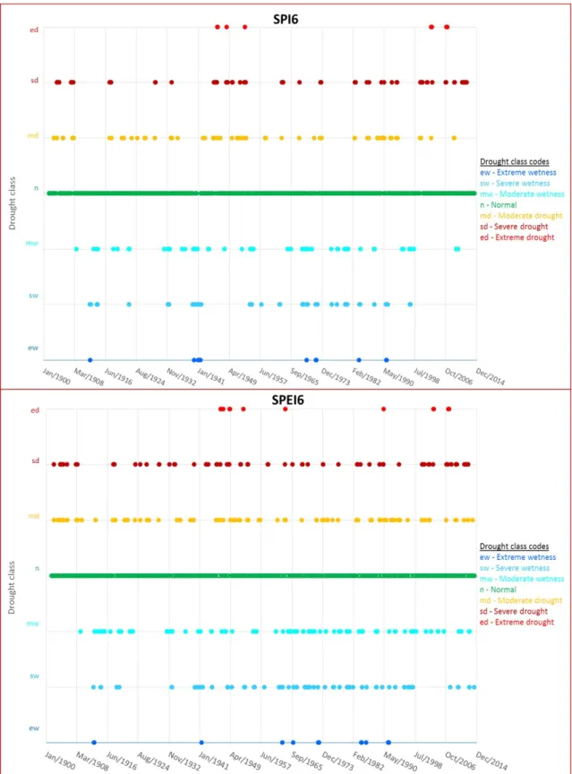
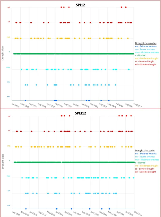
The temporal evolution of the original drought and wetness classes for the study period is shown in Figure2(SPEI6) and Figure3(SPEI12), considering the classification proposed by McKee et al. [39] with seven categories (Table1). In these graphs, the statistical mode is considered since we are working with categorical variables (the SPEI classes) and the mode retrieves the most frequent drought or wetness class in that month within the 15 grid points that constitute the Prut basin (Figure1). Consequently, the retrieval of the statistical mode results in a single class for each month and, as expected, most of the months were categorized as ‘normal’ as can be seen by the dense green line in Figures2and3.
Water 2018, 10, 65 10 of 24
Water 2018, 10, 65 10 of 24
Figure 2. Most frequent classes by month for SPI6 and SPEI6. Figure 2.Most frequent classes by month for SPI6 and SPEI6.
Water 2018, 10, 65 11 of 24
Figure 3. Most frequent classes by month for the SPI12 and SPEI12.
When comparing the SPI6 with the SPEI6 (Figure 2), it is evident that the SPEI6 identifies slightly more severe and extreme droughts than the SPI6. The same seems to happen for severe and extreme wetness conditions. Regarding the temporal 12-month time scale (Figure 3), the same is true but the difference between both is slighter.
The full period range 1901–2014 (114 years) of available data was divided into four similar length sub-periods of 28–29 years each: the first sub-period was from 1901 to 1930; the second sub-period was from 1931 to 1958; the third sub-period was from 1959 to 1986, and the fourth sub-period was from 1987 to 2014. For each of the 15 grid points and 4 sub-periods, the number of times each class
Figure 3.Most frequent classes by month for the SPI12 and SPEI12.
When comparing the SPI6 with the SPEI6 (Figure2), it is evident that the SPEI6 identifies slightly more severe and extreme droughts than the SPI6. The same seems to happen for severe and extreme wetness conditions. Regarding the temporal 12-month time scale (Figure3), the same is true but the difference between both is slighter.
Water 2018, 10, 65 12 of 24
The full period range 1901–2014 (114 years) of available data was divided into four similar length sub-periods of 28–29 years each: the first sub-period was from 1901 to 1930; the second sub-period was from 1931 to 1958; the third sub-period was from 1959 to 1986, and the fourth sub-period was from 1987 to 2014. For each of the 15 grid points and 4 sub-periods, the number of times each class occurred was computed and the mean values compared between sub-periods. This division into four equal/similar sub-periods is done in order to obtain a reliable comparison of the drought class occurrences between sub-periods and because four is the minimum number of points necessary to find a curvature and its counter-curve and so to find an eventual cyclicity in drought class frequency. The analysis focused only on the sum of severe and extreme drought (classes sd + ed) and the sum of severe and extreme wetness classes (classes sw + ew) as these extreme classes are the ones with higher socio-economic impacts. The choice of joining classes sw and ew (and also classes sd and ed) results from the fact that the most extreme classes have only a few cases for the analyzed period and joining both classes will allow for a more robust analysis. Figure4presents the mean values of the occurrences for these sums of classes by the sub-period obtained for the SPEI6 (left) and the SPEI12 (right).
Water 2018, 10, 65 12 of 24
occurred was computed and the mean values compared between sub-periods. This division into four equal/similar sub-periods is done in order to obtain a reliable comparison of the drought class occurrences between sub-periods and because four is the minimum number of points necessary to find a curvature and its counter-curve and so to find an eventual cyclicity in drought class frequency. The analysis focused only on the sum of severe and extreme drought (classes sd + ed) and the sum of severe and extreme wetness classes (classes sw + ew) as these extreme classes are the ones with higher socio-economic impacts. The choice of joining classes sw and ew (and also classes sd and ed) results from the fact that the most extreme classes have only a few cases for the analyzed period and joining both classes will allow for a more robust analysis. Figure 4 presents the mean values of the occurrences for these sums of classes by the sub-period obtained for the SPEI6 (left) and the SPEI12 (right).
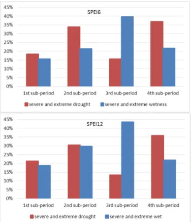
Figure 4. Mean frequencies of the 15 grid points for the occurrence of severe and extreme drought (red column) and severe and extreme wetness (blue column) in each sub-period for the SPEI6 and SPEI12.
Regarding the evolution of severe and extreme droughts (classes sd + ed), Figure 4 reveals an increase from the first to the second sub-period, followed by a decrease in the third sub-period and again an intense increase in the fourth sub-period. Concerning equivalent performance of severe and extreme wetness events (classes sw + ew) the behavior is different, showing an increase tendency from the first to the third sub-periods followed by a decrease in the fourth sub-period. Moreover, these distinct behaviors are similar for both the SPEI6 and SPEI12. To elucidate if the differences between the four sub-periods are statistically significant, a simple one-way analysis of variance (ANOVA) followed by a multiple comparison Turkey test [74] with a confidence level α = 0.05, was performed for each case (classes sd + ed and classes sw + ew, for both SPEI6 and SPE12).
Results for classes sd + ed of SPEI6 show that the increases in the number of severe and extreme drought occurrences from the first to second, first to fourth, and third to fourth sub-periods are statistically significant, as well as the decrease in number from the second to the third sub-periods. Between the first and the third and between the second and the fourth sub-periods, the differences are nonsignificant. With respect to the SPEI12, all changes between sub-periods are statistically significant, i.e., all the increases and decreases in the number of severe and extreme drought
Figure 4.Mean frequencies of the 15 grid points for the occurrence of severe and extreme drought (red column) and severe and extreme wetness (blue column) in each sub-period for the SPEI6 and SPEI12.
Regarding the evolution of severe and extreme droughts (classes sd + ed), Figure4reveals an increase from the first to the second sub-period, followed by a decrease in the third sub-period and again an intense increase in the fourth sub-period. Concerning equivalent performance of severe and extreme wetness events (classes sw + ew) the behavior is different, showing an increase tendency from the first to the third sub-periods followed by a decrease in the fourth sub-period. Moreover, these distinct behaviors are similar for both the SPEI6 and SPEI12. To elucidate if the differences between the four sub-periods are statistically significant, a simple one-way analysis of variance (ANOVA) followed by a multiple comparison Turkey test [74] with a confidence level α = 0.05, was performed for each case (classes sd + ed and classes sw + ew, for both SPEI6 and SPE12).
Results for classes sd + ed of SPEI6 show that the increases in the number of severe and extreme drought occurrences from the first to second, first to fourth, and third to fourth sub-periods are statistically significant, as well as the decrease in number from the second to the third sub-periods. Between the first and the third and between the second and the fourth sub-periods, the differences are nonsignificant. With respect to the SPEI12, all changes between sub-periods are statistically significant, i.e., all the increases and decreases in the number of severe and extreme drought occurrences are statistically significant. These results point to an overall increase from the first to the fourth sub-periods but also to a strong multi-decadal evolution with possible cyclicity of the severe and extreme drought frequency in the Prut basin. In particular, if we restrict ourselves to the last 50–60 years (corresponding to the third and fourth sub-periods) the notorious rise from the third to the fourth sub-period is corroborated by several studies that reveal significant positive trends in drought frequency, severity, and duration for the Mediterranean and Carpathian region [6,7,19]. However, when using a longer span period, a study regarding Portugal also agrees with the hypothesis that severe and extreme droughts may present a cyclic component with the duration ranging from 26 to 30 years [75].
Concerning the number of severe and extreme wetness events (classes sw + ew) for SPEI6, ANOVA results reveal a statistical significance between all the sub-periods except between the second and the fourth. For the SPEI12, the exceptions (nonsignificant differences) occur between the first and the fourth and the second and the fourth sub-periods. Therefore, these finds point to a significant increase in severe and extreme wetness events from the first period to the third and then a significant decrease in the last sub-period. Apart from some minor differences, the results obtained for the SPI are similar to those attained for SPEI and are not presented for the sake of simplicity.
3.2. Prediction Analysis
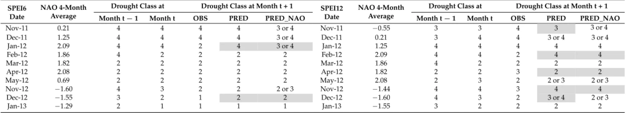
A comparison between the observed the SPEI6 (or SPEI12) drought class at month t + 1 (from now on denoted as OBS) and the prediction using the modeling with and without the NAO influence (from now on denoted respectively as PRED and PRED_NAO) was performed for each grid point (Figure1, Table3). In order illustrate the prediction made for each grid point, an example is presented in Tables6 and7for two distinct temporal periods. In those tables the comparison between the observed SPEI6 (or SPEI12) drought class at month t + 1 (OBS), and the prediction using the modeling with and without the NAO influence (PRED and PRED_NAO) for a chosen grid point is shown for two periods, respectively from January 2012 to June 2013 (Table6) and the extended winter months between 2011 and 2013 (Table7). The observed SPEI6 (SPEI12) drought class at months t−1 and t, as well as the average NAO value for the last four months considered in the modeling are also shown. It should be noted that the period selected for the comparison refers to a period with several class changes involving all four drought classes. When two drought classes are equally probable, then the predicted drought class is identified for instance as “1 or 2”, indicating that the transition probabilities into either class 1 or class 2 are similar. The cells in Tables6and7are highlighted in grey when the predictions do not match the observations.
Water 2018, 10, 65 14 of 24
Table 6.The SPEI6 and SPEI12: Comparison between observed (OBS) and predicted drought class transitions (with and without the NAO influence, “PRED” and “PRED_NAO”, respectively) for grid point 13 (Table3) during the period from January 2012 to June 2013.
SPEI6 Date
NAO 4-Month Average
Drought Class at Drought Class at Month t + 1 SPEI12 Date
NAO 4-Month Average
Drought Class at Drought Class at Month t + 1
Month t − 1 Month t OBS PRED PRED_NAO Month t − 1 Month t OBS PRED PRED_NAO
Jan-12 2.09 4 4 2 4 3 or 4 Jan-12 1.25 4 4 4 4 4 Feb-12 1.86 4 2 2 2 2 Feb-12 2.09 4 4 2 4 4 Mar-12 1.82 2 2 2 2 2 Mar-12 1.86 4 2 2 2 2 Apr-12 2.08 2 2 2 2 2 Apr-12 1.82 2 2 3 2 2 May-12 0.69 2 2 2 2 2 May-12 2.08 2 3 2 2 or 3 2 or 3 Jun-12 −0.03 2 2 4 2 2 Jun-12 0.69 3 2 4 2 2 Jul-12 −1.00 2 4 3 4 3 or 4 Jul-12 −0.03 2 4 3 3 or 4 3 or 4 Aug-12 −1.77 4 3 4 2 3 or 4 Aug-12 −1.00 4 3 4 2 or 3 3 or 4 Sep-12 −1.29 3 4 4 3 or 4 3 or 4 Sep-12 −1.77 3 4 4 3 or 4 3 or 4 Oct-12 −1.44 4 4 3 4 3 or 4 Oct-12 −1.29 4 4 4 4 4 Nov-12 −1.60 4 3 2 2 3 or 4 Nov-12 −1.44 4 4 3 4 4 Dec-12 −1.55 3 2 1 2 2 Dec-12 −1.60 4 3 2 2 or 3 3 or 4 Jan-13 −1.29 2 1 1 1 1 Jan-13 −1.55 3 2 2 2 2 Feb-13 −0.66 1 1 1 1 or 2 1 or 2 Feb-13 −1.29 2 2 2 2 2 Mar-13 0.08 1 1 2 1 or 2 1 or 2 Mar-13 −0.66 2 2 1 2 2 Abr-13 −0.58 1 2 2 2 2 Apr-13 0.08 2 1 2 1 1 or 2 May-13 −0.73 2 2 2 2 2 May-13 −0.58 1 2 2 2 2 Jun-13 −0.69 2 2 2 2 2 Jun-13 −0.73 2 2 2 2 2
Table 7.The SPEI6 and SPEI12: Comparison between observed (OBS) and predicted drought class transitions (“PRED” and “PRED_NAO”) for grid point 13 (Table3) during the periods November 2011 to May 2012, November 2012 to May 2013, and November 2013 to December 2013.
SPEI6 Date
NAO 4-Month Average
Drought Class at Drought Class at Month t + 1 SPEI12 Date
NAO 4-Month Average
Drought Class at Drought Class at Month t + 1
Month t − 1 Month t OBS PRED PRED_NAO Month t − 1 Month t OBS PRED PRED_NAO
Nov-11 0.21 4 4 4 4 3 or 4 Nov-11 −0.55 3 3 4 3 3 or 4 Dec-11 1.25 4 4 4 4 3 or 4 Dec-11 0.21 3 4 4 3 or 4 3 or 4 Jan-12 2.09 4 4 2 4 3 or 4 Jan-12 1.25 4 4 4 4 4 Feb-12 1.86 4 2 2 2 2 Feb-12 2.09 4 4 2 4 4 Mar-12 1.82 2 2 2 2 2 Mar-12 1.86 4 2 2 2 2 Apr-12 2.08 2 2 2 2 2 Apr-12 1.82 2 2 3 2 2 May-12 0.69 2 2 2 2 2 May-12 2.08 2 3 2 2 or 3 2 or 3 Nov-12 −1.60 4 3 2 2 2 or 3 Nov-12 −1.44 4 4 3 4 4 Dec-12 −1.55 3 2 1 2 2 Dec-12 −1.60 4 3 2 3 or 4 2 or 3 Jan-13 −1.29 2 1 1 1 1 Jan-13 −1.55 3 2 2 2 2
Table 7. Cont. SPEI6
Date
NAO 4-Month Average
Drought Class at Drought Class at Month t + 1 SPEI12 Date
NAO 4-Month Average
Drought Class at Drought Class at Month t + 1
Month t − 1 Month t OBS PRED PRED_NAO Month t − 1 Month t OBS PRED PRED_NAO
Feb-13 −0.66 1 1 1 1 or 2 1 or 2 Feb-13 −1.29 2 2 2 2 2 Mar-13 0.08 1 1 2 1 or 2 1 or 2 Mar-13 −0.66 2 2 1 2 2 Apr-13 −0.58 1 2 2 2 2 Apr-13 0.08 2 1 2 3 or 4 3 or 4 May-13 −0.73 2 2 2 2 2 May-13 −0.58 1 2 2 2 2 Nov-13 0.94 2 2 2 2 2 Nov-13 1.38 2 2 2 2 2 Dec-13 0.32 2 2 2 2 2 Dec-13 0.94 2 2 2 2 2
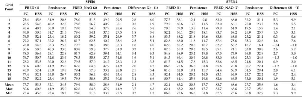
Table 8.Proportion correct (PC) and Heidke skill score (HSS) (%) for the SPEI6 and SPEI12 modeling in the extended winter months for PRED (1) and its fractional improvement over the persistence forecast; for PRED_NAO (2) and its fractional improvement over the persistence forecast; and for the difference between both modeling approaches.
Grid Point
SPEI6 SPEI12
PRED (1) Persistence PRED_NAO (2) Persistence Difference: (2)−(1) PRED (1) Persistence PRED_NAO (2) Persistence Difference: (2)−(1)
PC HSS PC HSS PC HSS PC HSS PC HSS PC HSS PC HSS PC HSS PC HSS PC HSS 1 75.4 45.6 31.9 20.8 78.0 51.5 39.2 29.5 2.6 6.0 77.7 58.1 12.1 9.8 83.0 68.0 32.2 31.1 5.3 9.9 2 78.5 54.8 40.2 32.3 78.8 56.7 40.9 35.1 0.3 1.9 79.2 60.6 13.3 11.5 82.0 66.1 25.0 23.7 2.8 5.5 3 76.4 48.2 30.0 19.3 79.0 54.0 37.9 28.4 2.6 5.8 78.5 59.8 13.8 11.4 79.9 61.9 19.5 15.9 1.4 2.1 4 76.8 50.5 31.7 21.5 78.6 54.1 37.5 27.5 1.8 3.6 82.2 66.1 20.6 18.1 83.7 69.2 26.9 25.7 1.5 3.1 5 76.5 52.4 23.4 18.2 80.2 59.2 35.1 29.9 3.7 6.8 83.5 68.2 21.8 19.6 83.8 68.8 23.2 21.1 0.3 0.6 6 79.2 57.1 32.2 26.2 81.7 62.5 40.2 35.4 2.5 5.4 82.8 68.0 11.8 11.7 87.4 75.6 35.3 32.6 4.6 7.6 7 78.0 54.3 33.3 25.5 79.7 58.3 38.8 32.3 1.8 4.0 82.6 67.2 20.5 18.7 82.2 66.2 18.7 16.4 −0.4 −1.0 8 80.6 58.5 40.3 33.0 80.8 59.8 37.9 31.9 0.2 1.3 82.5 65.9 20.3 18.5 85.1 71.1 32.0 30.8 2.6 5.2 9 78.3 56.6 28.1 22.8 81.7 62.9 39.4 34.1 3.4 6.3 84.8 68.9 23.2 19.8 87.5 73.9 36.8 32.9 2.7 5.0 10 76.7 50.7 32.8 23.9 78.3 55.8 37.5 31.8 1.6 5.1 84.3 69.4 30.9 26.8 83.0 68.4 25.3 24.6 −1.3 −1.0 11 78.2 53.5 30.0 22.6 79.5 57.0 34.2 28.3 1.3 3.5 81.7 64.5 17.8 15.3 82.6 66.5 21.8 20.1 0.9 2.0 12 80.6 60.6 41.9 35.0 82.6 64.8 47.9 41.9 2.0 4.2 86.8 72.6 36.8 31.8 85.6 70.8 30.7 27.4 −1.2 −1.8 13 76.9 52.4 25.0 19.8 79.4 57.8 33.2 28.8 2.5 5.4 81.6 62.8 19.1 15.7 84.4 68.9 31.5 29.4 2.8 6.1 14 77.4 52.1 35.8 26.7 80.2 56.4 43.6 33.4 2.8 4.3 82.4 64.5 20.2 16.5 83.1 66.9 23.7 22.2 0.7 2.4 15 76.7 52.2 25.4 19.5 79.8 58.8 35.2 30.8 3.1 6.6 80.7 61.4 25.6 19.8 82.6 66.5 33.0 30.4 1.9 5.1 Mean 77.7 53.3 32.1 24.5 79.9 58.0 38.6 31.9 2.1 4.7 82.1 65.2 20.5 17.7 83.7 68.6 27.7 25.6 1.6 3.4 Max 80.6 60.6 41.9 35.0 82.6 64.8 47.9 41.9 3.7 6.8 82.1 65.2 20.5 17.7 83.7 68.6 27.7 25.6 1.6 3.4 Min 75.4 45.6 23.4 18.2 78.0 51.5 33.2 27.5 0.2 1.3 86.8 72.6 36.8 31.8 87.5 75.6 36.8 32.9 5.3 9.9
Water 2018, 10, 65 16 of 24
From the analysis of these tables, it may be observed that the modeling performs very well in predicting the maintenance of the drought classes, but not particularly well when a change of class occurs (decrease or increase of the drought class category) breaking with the drought class established in the preceding two months. Furthermore, for the example shown in Tables6and7, we can see that it seems more difficult to predict a class decrease or increase when using the SPEI12 than the SPEI6, likely due to the SPEI6 having quicker response to the variability of precipitation in periods with frequent changes of drought classes. Besides that, when comparing Tables6and7, some decrease in the number of disagreements is perceived for the case that considers the modeling restricted to the extended winter months: this probably due to the slightly higher magnitude of the correlations between NAO and SPEI for the wetter months. Finally, the agreements between the predictions and observations are a little higher when the “PRED_NAO” modeling is used instead of just “PRED”, for both the SPEI6 and SPEI12, indicating that some cases of class change could be better predicted with the “PRED_NAO”, namely those with negative NAO. Results for the other grid points can present some variability, but the overall behavior will not show significant differences. This analysis was repeated for all the grid points in Figure1and the results were aggregated.
To assess the performance of the log-linear modeling influenced by the NAO comparative to modeling without that influence and the percentage of improvement of both modeling over the persistence forecast, the proportion correct (PC) and Heidke skill score (HSS) were computed for the entire period of the time series as explained in Section2.3. The results corresponding to the SPEI6 and the SPEI12 modeling of the extended winter months are shown in Table8, respectively. For the SPI6 and SPI12, as well as for the modeling of all the months of the year, only the mean, maximum, and minimum values are presented instead of the results per grid point (Tables9–11) for the sake of simplicity.
To better visualize the performance of the log-linear modeling without and with the NAO influence, graphical representations of the PC and HSS skill score results are presented in Figures5–8. In those figures, it is shown for the SPEI6 (SPI6) (above) and SPEI12 (SPI12) (bellow) the PC (left) and HSS (right) the improvement of the “PRED_NAO” over the “PRED” forecast, corresponding to the difference between both. In some cases, there is no improvement in certain grid points, indeed there is a decrease.
The information given in Tables8–11allows us to conclude that the log-linear modeling performs consistently better than the persistence forecast, indicating that the model can predict more accurately than the simple maintenance of the drought class of the preceding month, that is, a considerable number of class changes are well predicted.
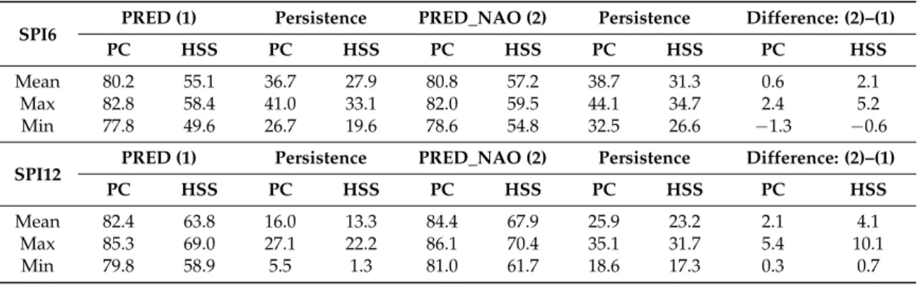
Table 9.Mean, maximum and minimum of the PC and HSS skill scores (%) for the SPI6 (above) and SPI12 (below) for the extended winter months.
SPI6 PRED (1) Persistence PRED_NAO (2) Persistence Difference: (2)–(1)
PC HSS PC HSS PC HSS PC HSS PC HSS
Mean 80.2 55.1 36.7 27.9 80.8 57.2 38.7 31.3 0.6 2.1 Max 82.8 58.4 41.0 33.1 82.0 59.5 44.1 34.7 2.4 5.2 Min 77.8 49.6 26.7 19.6 78.6 54.8 32.5 26.6 −1.3 −0.6
SPI12 PRED (1) Persistence PRED_NAO (2) Persistence Difference: (2)–(1)
PC HSS PC HSS PC HSS PC HSS PC HSS
Mean 82.4 63.8 16.0 13.3 84.4 67.9 25.9 23.2 2.1 4.1 Max 85.3 69.0 27.1 22.2 86.1 70.4 35.1 31.7 5.4 10.1 Min 79.8 58.9 5.5 1.3 81.0 61.7 18.6 17.3 0.3 0.7
Table 10.As in Table9but relative to all months and SPEI6 (above) and SPEI12 (below).
SPEI6 PRED (1) Persistence PRED_NAO (2) Persistence Difference: (2)–(1)
PC HSS PC HSS PC HSS PC HSS PC HSS
Mean 78.7 54.8 33.5 25.7 79.1 56.0 34.2 27.2 0.3 1.2 Max 82.5 62.7 41.3 33.9 81.1 60.6 41.9 34.5 2.5 6.4 Min 75.4 44.8 24.9 17.1 76.4 51.2 24.7 18.9 −2.5 −4.9
SPEI12 PRED (1) Persistence PRED_NAO (2) Persistence Difference: (2)–(1)
PC HSS PC HSS PC HSS PC HSS PC HSS
Mean 81.6 64.0 18.2 15.5 82.6 65.9 22.5 20.0 1.0 1.9 Max 83.8 68.2 29.2 25.6 84.3 69.6 26.5 23.0 2.5 5.2 Min 79.5 60.6 7.6 6.1 80.9 62.8 16.9 15.7 −0.6 −1.2
Table 11.As in Table9but relative to all months and SPI6 (above) and SPI12 (below).
SPI6 PRED (1) Persistence PRED_NAO (2) Persistence Difference: (2)–(1)
PC HSS PC HSS PC HSS PC HSS PC HSS
Mean 79.0 52.0 34.0 24.3 80.2 54.5 37.8 28.3 1.2 2.5 Max 81.6 57.1 41.2 32.2 82.8 60.0 45.0 37.0 5.0 9.2 Min 75.3 44.0 23.4 13.6 78.5 48.5 32.0 20.8 −0.6 −2.0
SPI12 PRED (1) Persistence PRED_NAO (2) Persistence Difference: (2)–(1)
PC HSS PC HSS PC HSS PC HSS PC HSS
Mean 81.8 62.3 19.0 15.6 82.4 63.4 21.6 18.8 0.6 1.1 Max 84.6 66.8 25.8 21.2 85.2 69.1 34.1 29.4 4.0 6.1 Min 79.4 57.7 7.3 6.2 80.4 59.6 15.7 14.7 −1.6 −1.9
Water 2018, 10, 65 18 of 24
Figure 5. PC and HSS improvement (%) considering the influence of NAO on the SPEI6 and SPEI12
modeling for the extended winter months for each of the 15 grid points.
Figure 6. PC and HSS improvement (%) considering the influence of NAO on the SPI6 and SPI12
modeling for the extended winter months for each of the 15 grid points.
Figure 5.PC and HSS improvement (%) considering the influence of NAO on the SPEI6 and SPEI12 modeling for the extended winter months for each of the 15 grid points.
Water 2018, 10, 65 18 of 24
Water 2018, 10, 65 18 of 24
Figure 5. PC and HSS improvement (%) considering the influence of NAO on the SPEI6 and SPEI12
modeling for the extended winter months for each of the 15 grid points.
Figure 6. PC and HSS improvement (%) considering the influence of NAO on the SPI6 and SPI12
modeling for the extended winter months for each of the 15 grid points.
Figure 6. PC and HSS improvement (%) considering the influence of NAO on the SPI6 and SPI12 modeling for the extended winter months for each of the 15 grid points.
Water 2018, 10, 65 19 of 24
Figure 7. PC and HSS improvement (%) considering the influence of NAO on the SPEI6 and SPEI12
modeling for all months for each of the 15 grid points.
Figure 8. PC and HSS improvement (%) considering the influence of NAO on the SPI6 and SPI12
modeling for all months for each of the 15 grid points.
Figure 7.PC and HSS improvement (%) considering the influence of NAO on the SPEI6 and SPEI12 modeling for all months for each of the 15 grid points.
Water 2018, 10, 65Figure 7. PC and HSS improvement (%) considering the influence of NAO on the SPEI6 and SPEI12 19 of 24
modeling for all months for each of the 15 grid points.
Figure 8. PC and HSS improvement (%) considering the influence of NAO on the SPI6 and SPI12
modeling for all months for each of the 15 grid points.
Figure 8. PC and HSS improvement (%) considering the influence of NAO on the SPI6 and SPI12 modeling for all months for each of the 15 grid points.
Furthermore, better overall performances are obtained when the modeling is applied to the 12-month time scale (average range PC: 82–84; HSS: 62–69), in contrast with the 6-month time scale (average range PC: 77–80; HSS: 52–58) (Tables8–11, Figures5–8). This is likely to be related to the less frequent change of classes within the 12-month time scale and favors the ability of easily identifying capturing the behavior of changes in drought classes in the preceding months.
When the modeling is restricted only to the extended winter months instead of all months of the year, higher skill scores are obtained in most of the cases (Figure5vs. Figure7, Figure6vs. Figure8), the increase being however not very expressive (Table8vs. Table10, Table9vs. Table11). The relatively small increase of the correlation coefficient between the SPEI (SPI) and the NAO when considering only the extended winter months over all the months of the year may justify these small gains in the skill scores.
Concerning the introduction of the NAO predictor in the modeling, the highest improvements obtained in the skill scores with the “PRED_NAO” are obtained when modeling the extended winter months of the SPEI6 and SPI12 (Figures5and6). Those improvements are however not impressive, which may be due to the low correlations between the SPEI (SPEI) and the NAO index (Table3). They range between 0.2 and 3.7 (PC) and between 4.7 and 6.8 (HSS) for the SPEI6, and between 0.3 and 5.4 (PC) and between 4.1 and 10.1 (HSS) for the SPI12 (Tables8and9, Figures5and6). For the other cases, there are several grid points for which there is no improvement, i.e., the inclusion of the NAO influence does not bring any benefit. This situation may be justified by the fact that when modeling the drought classes transitions separately (NAO+ and NAO−), the accuracy of the prediction is somewhat diminished in comparison with modeling without the NAO because the data is divided into two groups with about half of the observations each. This accuracy reduction is not strongly compensated by the relatively low correlations, resulting in minor improvements of the predictions with the model “PRED_NAO” and occurs mainly for the transitions that imply a jump of 2 or 3 in the drought category,
Water 2018, 10, 65 20 of 24
Regarding the SPEI versus SPI comparison, no significant differences in terms of performance are found, since sometimes better performances are obtained for the SPEI, but the opposite also occurs (Figure5vs. Figure6, Figure7vs. Figure8).
The same modeling was applied to data from Portugal [63], however, there are several differences between both studies that do not allow a true comparison. First, just the SPI6 and SPI12 for all months of the year were modeled. Then, the NAO value considered in the PRED_NAO was not the mean of the four months before, but the value at the month t−l, where l is the lag that maximizes the correlation between the SPI and NAO. The skill scores obtained in that study are a little higher than the ones obtained herein, and the improvements in the predictions brought by the NAO introduction are also a bit larger, which is in agreement with the higher correlations between the SPI and the NAO for Portugal.
4. Conclusions
Monthly predictability of the SPEI and SPI drought classes under the influence of NAO was studied for the Prut basin using three-dimensional log-linear models, which are probabilistic models that learn from the preceding two months with the aim of predicting the drought class in the following month. These models have the ability to predict the persistence of the drought classes and some class changes that may be captured in the preceding two months. However, when a sudden change of class occurs (decrease or increase), it becomes particularly difficult to predict it, even when the NAO phase influencing the transition is known. Some reasons for that may be related to the not sufficiently high correlations between the SPEI (SPEI) and the NAO, for the Prut basin. However, some improvements in the predictions are obtained by the NAO introduction in the modeling, mainly when applied to the SPEI6 and the SPI12 and only to the extended winter months. Nevertheless, the overall performances of the log-linear modeling are good. Consequently, it can be concluded that the log-linear modeling has good performance skills when predicting the drought class one month ahead based on the information of drought classes of the two previous months. Nevertheless, this method presents the fragility of failing to predict many class transitions, which are different than the classes in the previous two months.
With respect to the drought class analysis the full study period was divided into four sub-periods of similar lengths. The findings, corroborated by other studies for the Mediterranean region, point to an overall increase in drought frequency from the first to the fourth sub-period but also to a strong multi-decadal evolution, with possible cyclicity of severe and extreme drought frequency in the Prut basin. In particular, for the last 50–60 years, the increment is very pronounced. Concerning the number of severe and extreme wetness events, the findings point to a significant increase from the first period to the third, and then a significant decrease in the last sub-period.
We believe that a methodology which can predict drought classes a few months in advance will beneficiate stakeholders, farmers, and also insurance companies so they are able to react accordingly and take proper action plans. In this sense, even with the mentioned limitations, we think the presented methodology can be part of an early warning system aiming to inform water users (especially farmers) in their water management decisions.
Acknowledgments:This work was partially supported by the projects IMDROFLOOD—Improving Drought and Flood Early Warning, Forecasting and Mitigation using real-time hydroclimatic indicators (WaterJPI/0004/2014) and project UID/MAT/00297/2013 (Centro de Matemática e Aplicações), both funded by funded by Fundação para a Ciência e a Tecnologia, Portugal (FCT). Ana Russo thanks also FCT by the Post-Doc research grant SFRH/BPD/99757/2014.
Author Contributions:E.M. conceived the work, performed the drought class calculations, analyzed the data, and wrote the paper; A.R. calculated the drought indicators, contributed to the materials and wrote the paper; and R.M.T. conceived the work, contributed to the materials, analyzed the data and wrote the paper.
Conflicts of Interest:The authors declare no conflict of interest. The founding sponsors had no role in the design of the study; in the collection, analyses, or interpretation of data; in the writing of the manuscript, and in the decision to publish the results.
![Figure 1. Map of Romania indicating the 15 grid points (from the Climatic Research Unit (CRU) database) covering the study area (delimited by a red line) and showing the Carpathians Mountains as well as the extra-Carpathian region [45] delimited here by a](https://thumb-eu.123doks.com/thumbv2/123dok_br/15460016.1030624/3.892.256.635.698.1046/indicating-climatic-research-delimited-carpathians-mountains-carpathian-delimited.webp)