RBRH, Porto Alegre, v. 23, e3, 2018 Scientiic/Technical Article
http://dx.doi.org/10.1590/2318-0331.0318170038
Performance of bioretention experimental devices: contrasting laboratory
and ield scales through controlled experiments
Performance de dispositivos experimentais de bioretenção: comparação entre escala de laboratório e de campo a partir de experimentos controlados
Marina Batalini de Macedo1, César Ambrogi Ferreira do Lago1, Eduardo Mario Mendiondo1 and
Vladimir Caramori Borges de Souza2
1Universidade de São Paulo, São Carlos, SP, Brazil 2Universidade Federal do Alagoas, Maceió, AL, Brazil
E-mails: marina_batalini@hotmail.com (MBM), cesar-lago@hotmail.com (CAFL), e.mario.mendiondo@gmail.com (EMM), vcaramori@yahoo.com (VCBS)
Received: March 20, 2017 - Revised: September 19, 2017 - Accepted: November 15, 2017
ABSTRACT
Studying the performance of LID devices on a laboratory scale has the advantage of lexible layouts, so that more factors can be tested.
However, they do not always correspond to what happens on a real scale of application. This paper focuses on a comparative analysis
between two bioretention experimental devices considering ield and laboratory scales. Based on this comparison, our understanding can be enhanced to extrapolate the results. Flow rate and duration were used as the main equivalence parameters. However, these parameters were insuficient to ensure similarity in the results. We proposed to include control volume, an application rate and an equivalent net depth as new parameters. Further research should test the variation of these parameters.
Keywords: SUDS; Stormwater control; Water retention; Pollutant removal.
RESUMO
Estudos da performance em laboratório possuem a vantagem de layouts lexíveis, podendo testar mais fatores. No entanto, nem sempre correspondem ao que acontece na escala real de aplicação. Este estudo foca em uma análise comparativa entre dispositivos experimentais de bioretenção em escala de campo e em escala de laboratório. A partir dessa comparação, é possível avançar na compreensão para extrapolação dos resultados. Como principais parâmetros de equivalência, foram utilizados a taxa de luxo e a duração. No entanto, observou-se que estes parâmetros foram insuicientes para garantia de similaridade nos resultados. Indicamos como novos parâmetros a serem incorporados o volume de controle, taxa de aplicação e altura equivalente útil. Novos estudos com a variação destes parâmetros devem ser feitos.
VARIABLES LIST
Aield = Surface area of bioretention device in ield [m];
Alab = Surface area of bioretention box in laboratory [m];
Aw = Surface receiving precipitation for the catchment
related to the bioretention in the ield [m2];
C(t) = Concentration, at time t [mg/L];
Fm = Average low rate [cm/h]; Hequivalent = Equivalent net depth [m];
Hgravel = Depth of the gravel layer [m];
Hsand = Depth of the sand layer [m];
Hsoil = Depth of the soil layer [m];
I(t) = Percolated low into the ground [L/min];
MI(t) = Iniltrated/treated pollutant mass by the LID
practice [g];
Min(t) = Pollutant mass in the inlow runoff [g];
Mout(t) = Pollutant mass in the outlow [g];
MP(t) = Pollutant mass in the precipitation, directly over
the bioretention basin [g];
Ms(t) = Stored pollutant mass, including positive or negative reactions due to internal processes, i.e. sorption,
degradation, etc., in the bioretention basin [g];
n = Total number of campaigns; P(t) = Precipitation [mm];
Q(t) = Water low at time t [L/min];
Qin(t) = Inlow discharge [L/min];
Qmed ield = Average inlow, in ield [L/h];
Qout(t) = Outlow discharge [L/min];
S(t) = Storage volume in the bioretention basin [L];
t = Analyzed time interval [min];
tield = Duration of the event in ield [h];
ti = Duration of campaign i [h];
Vcontrol = Control volume, equivalent with total inlet volume
[L];
Vi,total = Total inlet volume, considering campaign i [L];
∆t = Considered time interval [min].
INTRODUCTION
The rapid growth of cities and the lack of urban and territorial planning are causing an increase in soil sealing and,
consequently, an increase in runoff. As a result, traditional urban drainage systems are frequently overloaded, often leading to urban
loods. The extreme precipitation events are already a major cause
of natural disasters in Brazil (SANTOS, 2007; YOUNG; AGUIAR; SOUZA, 2015), causing loods, landslides, etc. In addition, according to the predictions of climate change, this scenario is likely to become worse (VALVERDE; MARENGO, 2010; MARENGO et al., 2010). Therefore, low impact development (LID) practices have appeared as alternative and sustainable systems for urban drainage, capable of reducing runoff at the
source, reestablishing the iniltration of water into the soil and
reducing social and environmental impacts.
LID practices include different approaches, ranging from participatory planning, environmental education and runoff reducing devices (FLETCHER; ANDRIEU; HAMEL, 2013). These devices can be used on many scales, such as source control, micro and macro drainage (MARSALEK; SCHREIER, 2009).
Examples could be green roofs, iniltration trenches, permeable
pavements, wetponds and bioretention cells (URBONAS; STAHRE, 1993; BAPTISTA; NASCIMENTO; BARRAUD, 2005; ERICKSON; WEISS; GULLIVER, 2013). In Brazil, recent studies have addressed the use of these devices, focusing mainly
on iniltration trenches and wells (LUCAS, 2011; LUCAS et al., 2015; GUTIERREZ, 2011). However, to broaden the knowledge of a greater number of devices, this paper outlines the operation of a bioretention system.
Bioretention systems have the dual function of qualitative and quantitative treatment, as they retain/detain the runoff while
removing pollutant loads. According to Erickson, Weiss and Gulliver (2013) and Laurenson et al. (2013), qualitative treatment occurs
through the physical-chemical process of iltration, sedimentation
and sorption, as well as the biological process of microbiological degradation and phytoremediation.
Considerable research efforts have been made to evaluate the bioretention system performance, prevailing studies on a laboratory scale. Wang et al. (2015, 2016) investigated metal removal
(Cd, Cu, Pb), testing different iltering media with experiments
conducted in bioretention columns. They found a removal rate above 90% in the percolation outlet. Rycewicz-Borecki, McLean and Dupont (2017) also evaluated the removal of metals Cu, Pb, and Zn,
carrying out experiments on a laboratory scale. Their results reported
metal removal above 92% and demonstrated accumulation in the macrophytes used to help the treatment. Nevertheless, studies conducted in the laboratory are not limited to metals. Chahal, Shi and Flury (2016), Liu et al. (2014) and Bratieres et al. (2008) evaluated the nutrient removal in a bioretention system and
reported removal eficiency ranging from 80 to 99%.
Field scale studies have also started to increase. Some examples
are listed here. In their paper, Mangangka et al. (2015) focused on how hydraulic and hydrologic factors affect the pollutant removal
in ield conditions in dry and rainy seasons. As a main result, they observed that the antecedent dry period has a great inluence on the nitriication and export process of nitrate. Petterson et al. (2016) and Lucke and Nichols (2015) investigated the removal of pathogens, nutrients and metals. For the pathogen removal, Petterson et al. (2016) observed that the removal performance
for microbial (viral, bacterial and protozoan) varied signiicantly
removal rates for total phosphorus, the only pollutant effectively removed from all basins investigated, and acceptable limits for metals in all basins, even after 10 years of operation. Davis (2007), Hatt, Fletcher and Deletic (2009), Winston, Luell and Hunt (2011) and Brown and Hunt (2012) found nutrient removal rates varying
from 3.2 to 64% and even nitrogen export – and removal rates
from 57 to 83% for metals.
Laboratory scale studies have some advantages: environmental conditions can be controlled to conduct a more in-depth investigation
of the treatment processes; and different factors that inluence the
treatment mechanisms can be used so as to identify the key-factor. In addition, there is no temporal dependence on the occurrence of storms and a greater amount of analyses can be made in a shorter time. However, what takes place in the laboratory will not
necessarily occur in the ield. In many cases, the results cannot be extrapolated without further analyses. When comparing the laboratory and ield studies mentioned here, it can be observed that laboratory experiments reported higher pollutant removal than ield experiments (around 90% and 60%, respectively).
Despite the importance of these studies developed in the
laboratory and in the ield, only a few have addressed the two scales of analysis in an integrated way. One example is a study
conducted by Hsieh and Davis (2005), which investigated the
removal rates in column experiments and bioretentions operating in the ield, evaluating the iltering media characteristics in their behavior. Their results demonstrate higher eficiencies for ield
systems when analyzing parameters of mineral contamination
(Pb and TSS) and higher eficiencies for the columns for parameters
that indicate nutrient contamination (TP, NH4, and NO2,3). Other studies have also made comparisons between column studies
in the laboratory with bioretention cells in the ield to evaluate speciic characteristics: Li and Davis (2008) evaluated the removal,
penetration and clogging of solid particles, using variable low
rates. Zhang et al. (2012) analyzed the effect of temperature on
the bacterial removal, irstly studying the behavior in the ield and
secondly varying the conditions in the column studies. They realized
that the results on a laboratory scale could not be extrapolated to the ield, because they presented different hydraulic dynamics.
Davis et al. (2006) tested another coniguration for a laboratory
experiment, in addition to the column test already widely used. In this study, the laboratory scale was made from bioretention box experiments with small and large dimensions. The irst one has closer dimensions to ield bioretention facilities, while the second one has more lexible characteristics for experimental variations, but with less similarity with the ield. The study was conducted in the laboratory and in the ield to evaluate the nutrient removal under controlled conditions, applying the same low rate (4.1 cm/h) and
the same duration. Despite the fact that they obtained variations between the results in the two scales, it could be concluded that
nitrate removal is small due to nitriication.
From the literature, it can be observed that even studies with integrated evaluation have a great variation in the results obtained
for the two scales, making it dificult to extrapolate and compare them. Moreover, these studies did not explain the reasons for the
differences and how to approach the comparison more assertively. Therefore, this paper focused on the development of
bioretention experimental devices in the laboratory and in the
ield, addressing the problems and limitations when comparing the
results for different scales. This can provide a better understanding and a step forward in raising the elements to make a better
extrapolation of the results obtained in the laboratory and future
integrated studies. In addition, considering that there are still few studies developed on bioretention in Brazil, this paper intends to
broaden the knowledge of this technique in a subtropical climate. Based on the controlled experiments, the hydraulic and qualitative treatment mechanisms can be identiied, as well as suggestions
for better sizing and design.
METHODOLOGY
Two experimental scales – laboratory and ield – were studied
in order to compare their performance results. The water and
pollutant mass balance quantiication, the study area characterization and how we determine the adequate low rate to ensure a similarity between the two scales are presented in the next sections.
Quali-quantitative data collection
To determine the system performance and eficiency,
the variables of the water and pollutant mass balance have to be determined numerically. In this study, the relevant variables
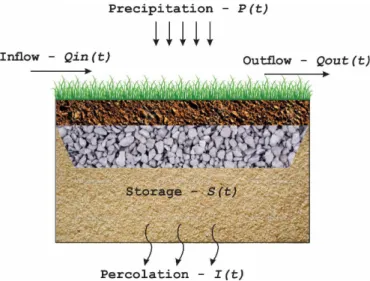
to determine the balances were inlow, outlow, stored volume, precipitated volume and percolation low, as shown in the diagram
(Figure 1). Equations 1 and 2 (adapted from ERICKSON; WEISS; GULLIVER, 2013) were used to quantify the water balance and mass balance, respectively.
( )=( in( ) + ( ) w)−
(
out( ) + ( ))
S t Q t t P t A Q t t I t t (1)
( )=( + )−
(
( )+ ( ))
s in P out I
M t M M M t M t (2)
where: Aw = Surface receiving precipitation for the catchment
related to the bioretention in the ield [m2]; I(t) = Percolated low
into the ground [L/min]; MI(t) = Iniltrated/treated pollutant
mass by the LID practice [g]; Min(t) = Pollutant mass in the
Figure 1. Bioretention diagram representing the laboratory and
inlow runoff [g]; Mout(t) = Pollutant mass in the outlow [g]; Ms(t) = Stored pollutant mass, including positive or negative reactions due to internal processes, i.e. sorption, degradation, etc., in the
bioretention basin [g]; MP(t) = Pollutant mass in the precipitation,
directly over the bioretention basin [g]; P(t) = Precipitation [mm]; Qin(t) = Inlow discharge [L/min]; Qout(t) = Outlow discharge
[L/min]; S(t) = Storage volume in the bioretention basin [L]; t = Analyzed time interval [min].
On a laboratory scale, quantitative and qualitative data were sampled manually every 5 min for inlow, outlow and percolation
(until there was no more percolation), and automatically for storage, using the humidity sensor TDR CS616 (Table 1).
The moisture sensor provides volume data of water fraction
for each corresponding sensor range. In this case, six sensors were
used, two related to the vegetated soil layer and four corresponding
to the iltering media (sand + gravel). The sensor ranges were
delimited according to their signal pickup radius, determined as 0.5 m and the boundaries of the layers. For each range, the moisture was converted to the volume of stored water by multiplying the fraction by the respective total volume of voids. Finally, the total stored volume was calculated as the sum of the value obtained for each range.
On the other hand, on the ield scale, the quantitative data was automatically collected, using a level sensor HOBO-WATER
U20L-02 (Table 1). For the inlow and outlow, the level sensor was associated with a weir (composite section and triangular
section), so that the low could be quantiied. For storage, the
level sensors were installed inside the piezometers presently found along the bioretention device. This method can calculate the
stored volume converted to a liquid level within the bioretention
cell, but may underestimate the total amount, as it disregards the water retention in the pores (in the form of moisture). As for the
qualitative sample collection, for the inlow, an automatic sampler
with a time interval of 5 min was used and for the storage and
outlow, the samples were collected manually with a time interval of 10 min, until there was no more outlow.
The difference between the two acquisition methods
adopted for the storage calculation on the laboratory and in the
ield scale will be analyzed in the Results and Discussion section.
To simulate the diffuse pollution in the runoff, a synthetic
low was made from the collection of solid particles found in the
pavements relative to each catchment, according to the methodology proposed by Maglionico (1998). The contaminants were collected by sweeping the pavement which had a greater accumulation of
sediment, predetermined and ixed for all the collections (red lines
in Figure 2). The antecedent dry period for each collection was determined, in order to relate the accumulation of sediments with
the period without rain. Subsequently, the collected contaminant particles were mixed with well water (without additional chlorine)
in tanks containing the total input volume to prepare the synthetic
low. The tanks were kept at a constant mixture throughout the
duration of the experiment. For this study, this efluent preparation
method was chosen because it is cheaper than preparing it by reagents, it has a simpler application and it resembles the real conditions of the catchment area, although there is no need for ensuring complete representativeness.
The water quality parameters analyzed were selected
to represent organic matter contamination - chemical organic
demand (COD) and total organic carbon (TOC) – nutrient
contamination - nitrite (NO2), nitrate (NO3), ammonia (NH3) e
phosphate (PO4) – solid contamination - sedimentable solids (SS) – and metals contamination - iron (Fe), zinc (Zn) and cadmium
(Cd). The analysis follows the methods proposed in the Standard
Methods for Examination of Water and Wastewater (APHA, 1992). For each variable of the pollutant mass balance, the total
load was quantiied according to Equation 3, integrating the total
time of the analyzed hydrographs.
( ) ( ) ( ) ( )
= ∫ = ∑ ∆
Load C t Q t dt C t Q t t (3)
where: C(t) = Concentration, at time t [mg/L]; Q(t) = Water low
at time t [L/min]; ∆t = Considered time interval [min].
Study area and experimental scales.
The two devices are situated in São Carlos, SP, Brazil at the University of Sao Paulo campus (USP campus 1 and 2) (Figure 2). For each one of the scales, the catchment was delimitated and,
consequently, the contribution area for the diffuse pollution. Table 1
presents the speciic characteristics for both scales.
In this characterization stage, we also established the parameter equivalent net depth (Hequivalent), deined as a height value
equivalent to the actual zone of the bioretention responsible for the qualitative treatment. This value is calculated from the ratio
of the net storage volume through the bioretention surface area. That is, this parameter represents a proportion between the net
retention capacity of the device inside the iltering media and its
application surface area, which will receive the runoff, resulting in
a value representing the real treatment zone within the technique. Therefore, higher values represent larger zones and, consequently,
greater treatment capacity. The Hequivalent was deined as a way to
standardize and parameterize the measurement of the qualitative treatment zone of a bioretention, regardless of its coniguration, scale and type of iltering material.
For the laboratory scale, a bioretention box experiment with small dimensions (1 m x 1 m x 1.45 m), according to those proposed
by Davis et al. (2006), was constructed to better evaluate the
key-factors that play an important role in the eficiency of a bioretention
practice. In this scale, the Hequivalent calculated is 0.32 m, as observed in Table 1. The laboratory device consists of three layers, the irst of which is a natural soil - predominantly sandy -, serving as a
medium for vegetation ixation (garden grass, Axonopus compressus),
Table 1. Speciications of the experimental scales analyzed.
Surface
area (m2)
H soil
(m)
H gravel
(m)
H sand
(m)
Hequivalent = Storage/Surface area
(m3/m2)
followed by gravel and sand, according to the arrangement shown in Figure 1. This iltering media was chosen to achieve the dual
function of water retention and water qualitative treatment. For this
scale, the catchment area corresponding to the contribution in diffuse pollution is completed urbanized, with a high level of surface paving. The runoff was simulated using a tank-pump-dispenser
low system, mixed with the diffuse pollution collected, operating at constant low and adjusted to simulate selected rainfall intensity. The water balance variables monitored were: inlow Qin(t), outlow
Qout(t) and percolation I(t).
Regarding the ield scale, the bioretention device is situated
at USP campus 2. On this scale, the device receives a runoff of a catchment with a total area of 2.3 ha. For this dimension, a micro drainage scale is considered (Figure 2b). The area is still mostly characterized as crawling vegetation, having only a few pathways. Therefore, the main contributions to the runoff are the automobile and pedestrian ways and a waterproof area relative to the campus building. The bioretention device has a surface area of 60.63 m2 and 3.2 m depth (Table 1). From the ratio of net volume and surface area, a Hequivalent of 1.02 m was determined. This device
has the same iltering media composition as the laboratory scale
(gravel followed by sand, as shown in Figure 1) covered by local
natural soil, with a sandy-loamy feature. The supericial layer was
vegetated with Brachiaria sp., selected to maintain the landscape integration and soil stabilization. On this scale, the water balance
variables monitored were: precipitation P(t), inlow Qin(t), outlow Qout(t) and storage S(t).
The diffuse pollution was collected manually along a contribution area of 1.6 ha at USP campus 1 (Figure 2a – red line) for the laboratory scale and along the catchment area of 2.3 ha
for the bioretention in the ield (Figure 2b – red line), after a dry period, as proposed by Maglionico (1998) and described in the previous section.
Comparing the scales of analysis
Comparing the two experimental scales requires establishing an equivalence relation between them. For this study, we proposed this equivalence relation based on three main parameters: Precipitation equivalent to real events, Flow rate and Duration. In this section, each
one of these parameters will be explained. Figure 3 shows a scheme with the relations established between these three parameters
(precipitation equivalent to real events, low rate and duration)
and the two scales.
In order for the controlled experiments in the bioretention box to correlate with the real events occurring in the ield, calculations
were made to establish the values of precipitation equivalent to real events. Based on a computational simulation (BIRENICE method, ROSA, 2016) and ield data acquisition during rainfall events (3 events during 2015), values of the total depth precipitated
Figure 2. Study areas for laboratory scale (a) and ield scale (b). The diffuse pollution was collected in the pathways represented by
and total drained volume were determined, corresponding to
a small and strong event. These equivalent values were used as upper and lower limits to regulate the low rate in the laboratory controlled experiments, maintaining the proper correspondence to the surface area of the bioretention box (Alab).
After ensuring the relationship between the controlled events in the laboratory with the non-controlled events in the
ield (or real) for the variable drained volume, it was necessary to establish a correspondence with the controlled experiments in the ield. To accomplish this purpose, we set a ixed low rate as a comparison parameter, which was calculated by averaging the
low rate used on the laboratory scale, according to Equation 4.
( )
, / =
=∑ni 1 i total lab i
m
10 xV A xt
F
n
(4)
where: Fm = Average low rate [cm/h]; Alab = Surface area of
bioretention box in the laboratory [m]; n = Total number of campaigns; Vi,total = Total inlet volume, considering campaign i [L]; ti = Duration of campaign i [h].
Finally, after setting the low rate value to be used for the controlled event in the ield, it was necessary to establish the required
duration of the event. Equation 5 presents the calculations for this parameter, based on the maximum capacity water tank (used as
the control volume) and the surface area for the bioretention
device in the ield (Aield). The low rate was transformed into an average inlow relative to the duration determined (Equation 6) in order to facilitate the operation throughout the experiment.
= control
field
field m
10 xV
t
A x F (5)
= control
med field field V Q
t (6)
where: Fm = Average low rate [cm/h]; Qmed ield = Average inlow,
in ield [L/h]; Aield = Surface area of bioretention device in ield
[m]; Vcontrol = Control volume, equivalent with total inlet volume
[L]; tield = Duration of the event in ield [h].
Other studies addressing the laboratory and ield experiments
in an integrated way (HSIEH; DAVIS, 2005; DAVIS et al., 2006; LI; DAVIS, 2008; ZHANG et al., 2012) did not establish a correspondence relationship between the two scales of analysis.
We propose here a comparison based on the relationships between the equivalent precipitation, low rate and duration. Therefore, the
results for the two scales were evaluated and compared, showing the problems and variations found for this proposed method. Finally, suggestions for future comparative studies were presented.
Campaigns
Regarding the laboratory scale, six campaigns were made to evaluate the bioretention quali-quantitative eficiency. The inlow ranged from 691 L/h to 2667 L/h (equivalent to a low rate ranging from 47.5 cm/h to 183.9 cm/h, based on the bioretention box surface area) as presented in Table 2. For the irst four campaigns, only the water balance variables were monitored,
resulting in samples for the qualitative analysis only for campaigns
5 and 6. The samples were collected manually from the weir outlet
(outlow) and the tank that receives the percolation low. The total number of samples collected per campaign is speciied in Table 2.
Figure 3. Representative scheme of the equivalence relation between the laboratory and ield scale.
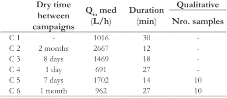
Table 2. Summary of campaigns on the laboratory scale.
Dry time between campaigns
Qin med
(L/h)
Duration
(min)
Qualitative Nro. samples
C 1 - 1016 30
-C 2 2 months 2667 12
-C 3 8 days 1469 18
-C 4 1 day 691 27
-C 5 7 days 1702 14 10
Different conditions of initial humidity in the iltering
media were also tested, varying the time interval between the campaigns from one day to two months (Table 2). During the
experiments, the room temperature was 25 °C ± 2.
For the ield scale study, the inlow was simulated in order to correspond with the average low rate, previously determined.
Then, a controlled event was conducted using a water tank truck serving as a reservoir. The total control volume was 10.12 m3, corresponding to a water depth of 0.43 mm and an average
inlow of 3157.8 L/h, or a low rate from 52.0 cm/h (based on
the bioretention device surface area).
Nine samples were collected to analyze the qualitative parameters on this scale: six samples were collected from the inlet,
representing the Min(t), and three samples were collected inside the storage, representing the MS(t). As the inlow simulation is done
with a control volume relative to P(t) and Qin(t) in a conjugated way, the incoming water quality represents the diffuse pollution
found in the runoff and in the direct incident rainfall, even if the latter has a small contribution. In this system, the percolation into
the ground is not collected, and consequently, it is not quantiied.
RESULTS AND DISCUSSION
Laboratory scale
Table 3 shows the water balance results for the bioretention
box on a laboratory scale. Except for campaign 2, the low rate and total volume applied were not suficient to completely saturate the iltering media and generate outlow in the weir. Only for campaign 2, there was a small outlow, which did not even
represent 1% of the total inlet volume. Therefore, considering all
the surveys, the mean water retention eficiency was 99.9% ± 0.2.
High percolation rates were also found, generally higher than 60%, achieving values of 73.7%. However, for campaigns 1 and 6,
this rate was less signiicant, achieving only 31.2% and 39.8%,
respectively. These two lower values occurred for the campaigns
that took place after a long dry period (≥ 1 month), so that the iltering media was completely dry and, therefore, with a higher
retention capability. Regarding campaign 2, even if it also occurred
after a long dry period (2 months), the mean low rate (Table 2) and total inlet volume (Table 3) were the greatest of all campaigns,
even leading to outlow. Therefore, it is possible that the iltering
media saturated faster, promoting percolation.
To complement the water balance analysis, Figure 4 shows the variation in time for each of the variables in all campaigns.
Considering the bioretention dimensions and a iltering media
porosity of 37%, the total net storage volume of the bioretention
box is around 500 L. However, the highest peak was found for
campaign 2, with a value close to 400 L, which means that the
storage peak did not reach the maximum value in any of the experiments. Nevertheless, the percolation hydrographs presented considerable peaks (25 L/min) and mean percolation rates for all the experiments. This result indicates that the water retention
capability of the system is affected not only by the net volume, but also by the hydraulic conductivity of the ground. Therefore, to calculate the system’s amortization capacity, these two factors
must be considered in the projects.
Still for campaign 2, in Figure 4 an outlow can be observed,
even though the inlet volume did not reach the maximum storage capacity. This can occur because the inlow exceeds the iniltration velocity into the bioretetion box, leading to a runoff in the box itself.
The percolation hydrographs and the temporal variation of storage (Figure 4) indicate a similar behavior between them, with the percolation peak occurring right after the storage peak.
From these results, it was also observed that the iltering media maintains the water storage even after the most signiicant
percolation has stopped, remaining almost constant after 120 min. Overall the results show that bioretention can help reestablish the water balance prior to urbanization (increasing water percolation rates in the ground). Additionally, this conclusion concerning the retention and detention process is important to
help sizing and design projects. If we consider the net volume
to be sized only as the difference of effective rainfall, or by
methods that consider differences between maximum volumes
(such as the rain-envelope method), an oversized value is found
and, consequently, higher costs.
To better evaluate the water storage process, Figure 5 was made showing the storage areas divided between the soil and sand layers, where the humidity sensors were installed. The soil layer
responds more quickly (storage peaks slightly before the sand layer) as it is the irst contact of the incoming low. The sand
layer, however, has a greater storage capacity in total volume and with a longer retention time.
In campaigns 5 and 6, in addition to the water balance analysis of the system, samples were collected to analyze the water
quality, increasing the system mass balance and the eficiency in
removing pollutants, for the percolation (Table 4).
Campaign 5 shows lower eficiency in removing TOC and higher eficiency for SS, followed by Zn. Regarding all the pollutants, an average range of removal eficiency can be observed,
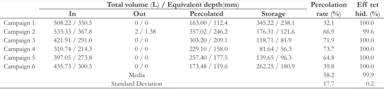
Table 3. Concentrated water balance. percolation rate and water retention eficiency for laboratory-scale campaigns.
Total volume (L) / Equivalent depth(mm) Percolation
rate (%)
Eff ret
hid. (%)
In Out Percolated Storage
Campaign 1 508.22 / 350.5 0 / 0 163.00 / 112.4 345.22 / 238.1 32.1 100.0 Campaign 2 533.33 / 367.8 2 / 1.38 357.02 / 246.2 176.31 / 121.6 66.9 99.6 Campaign 3 421.91 / 291.0 0 / 0 303.20 / 209.1 118.71 / 81.9 71.9 100.0 Campaign 4 310.74 / 214.3 0 / 0 229.10 / 158.0 81.64 / 56.3 73.7 100.0 Campaign 5 397.05 / 273.8 0 / 0 257.40 / 177.5 139.65 / 96.3 64.8 100.0 Campaign 6 435.73 / 300.5 0 / 0 173.48 / 119.6 262.25 / 180.9 39.8 100.0
Media 58.2 99.9
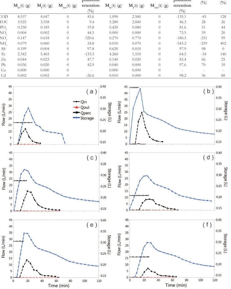
Figure 4. Temporal behavior of the variables’ inlow, outlow, storage and percolation in the bioretention box experiment, for:
(a) campaign 1; (b) campaign 2; (c) campaign 3; (d) campaign 4; (e) campaign 5 and (f) campaign 6.
Table 4. Mass balance and pollutant removal eficiency for the laboratory scale.
Campaign 5 Campaign 6
Average
(%)
SD
(%)
Total load Eff
pollution
retention
(%)
Total load Eff
pollution
retention
(%)
Min(t)(g) MI(t)(g) Mout(t)(g) Min(t)(g) MI(t)(g) Mout(t)(g)
COD 8.537 4.647 0 45.6 1.090 2.560 0 -135.1 -45 128
TOC 3.925 3.558 0 9.4 5.280 2.840 0 46.3 28 26
PO4 0.230 0.185 0 19.8 0.420 0.080 0 81.6 51 44
NO2 0.004 0.002 0 44.5 0.000 0.000 0 73.5 59 20
NO3 0.147 0.618 0 -320.6 0.270 0.770 0 -180.5 -251 99
NH3 0.079 0.060 0 24.8 0.010 0.070 0 -543.2 -259 402
SS 0.199 0.004 0 97.8 0.620 0.010 0 97.9 98 0
Fe 2.342 5.465 0 -133.3 4.260 1.510 0 64.5 -34 140
Zn 0.044 0.023 0 47.7 0.140 0.020 0 83.4 66 25
Pb 0.036 0.020 0 42.9 0.040 0.000 0 97.6 70 39
Cu 0.000 0.000 0 - 0.000 0.000 0 - -
varying from 20% to almost 50%. This range is low when compared to other studies which also evaluated the laboratory performance and obtained removal rates in the order of 90% (RYCEWICZ-BORECKI; MCLEAN; DUPONT, 2017; CHAHAL; SHI; FLURY, 2016; WANG et al., 2015, 2016; LIU et al., 2014; BRATIERES et al., 2008). Finally, an export of pollutants was found for NO3, Fe, and Cd. Fe export probably occurred due to
the local soil characteristics, which belong to the oxisol group
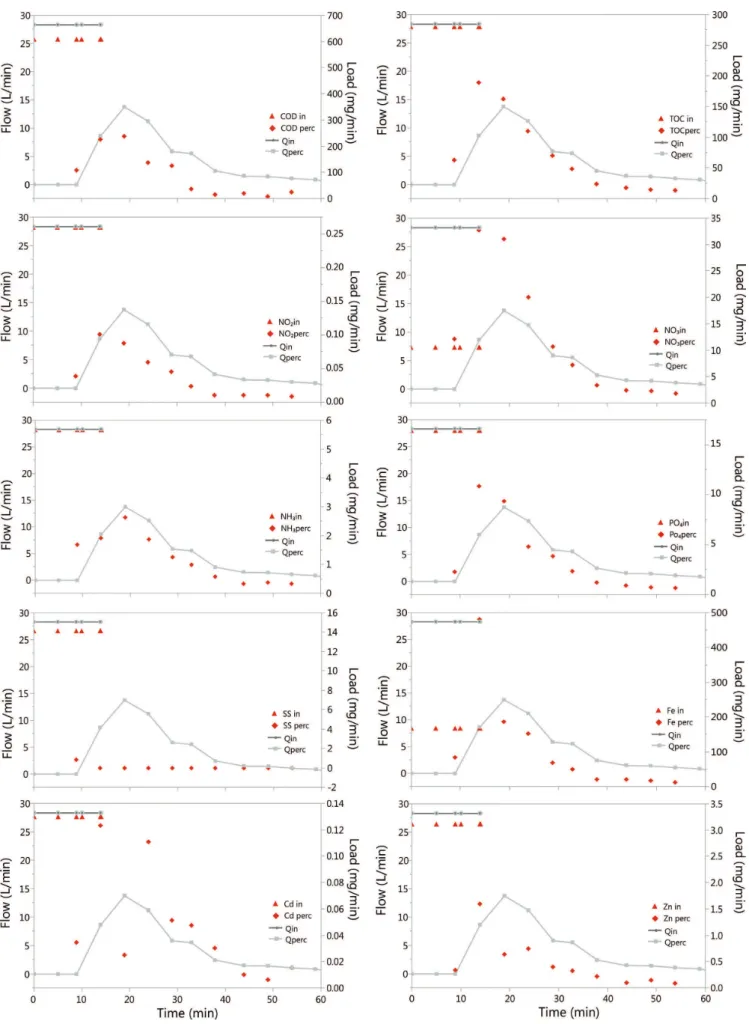
(characterized by high Fe content). The pollutograph of each pollutant is shown in Figure 6.
When analyzing the results for campaign 6, the lowest removal eficiency was also for TOC, with 46.3%. However, this
value was about 5x greater than for campaign 5. A similar behavior occurred for the other pollutants, except for those where we observed export. Despite the increase in removal eficiency when
compared to campaign 5, when compared to other laboratory scale studies (already cited) the value of the nutrient removal was still
low, not exceeding 82%. For the metals, the eficiency reached
values of 98.2%, close to the results observed in other studies. The pollutograph of each pollutant is shown in Figure 7. Still
regarding campaign 6, export was found for parameters COD,
NO3 and NH3.
NO3 export in both campaigns was observed. This behavior was also noted in other studies analyzing nutrients. Mangangka et al. (2015)
Figure 5. Storage capacity by layers of the bioretention box for: (a) campaign 1; (b) campaign 2; (c) campaign 3; (d) campaign 4;
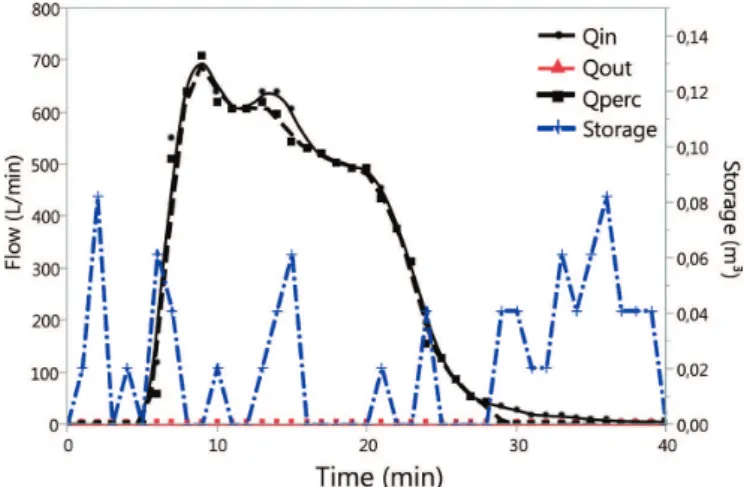
Figure 8. Temporal behavior of the variables’ inlow, outlow, storage and percolation, on a ield scale event.
analyzed the nitrogen series and they observed that the previously dry period had a primordial role in the treatment, especially for the nitrogen compounds. Long periods of drought contributed to reducing nitrite and ammonia at the device outlet, while it increased
the nitrate load, conirming the occurrence of the nitriication
process inside the bioretention. Moreover, Davis et al. (2006) and Hsieh, Davis and Needelman (2007) evaluated the nitrogen
removal in bioretention cells and observed nitrate export due to biotransformation and nitriication reactions.
For the other pollutants, the difference between the results
obtained from the two campaigns can also be explained by the different dry periods prior to the experiment. Campaign 5 took
place after 7 days of drought, while for campaign 6, this period was one month. Therefore, pollutant storage with no degradation in the small period between campaigns 4 and 5 may have occurred, which was then washed away by the percolation during campaign 5. Due to the greater drought time, this behavior did not happen
for campaign 6, justifying the greater removal eficiencies.
Field scale
Table 5 and Figure 8 present the water balance results for
the bioretention application on a ield scale. The results show no outlow, representing a water retention eficiency of 100%.
The bioretention device in the ield has a surface area of
60.63 m2, a total depth of 3.2 m, an average porosity of 37% and a storage capacity of 62 m3. Considering the control volume
used in the experiment (only 16% of the total net volume), the
storage data shows a negligible volume, not reaching even 0.12% of the total capacity. On the basis of this result, most of the inlet volume appears to percolate into the ground (percolation rate of
95.3%), with almost the same velocity and low. Figure 8 shows this behavior clearly since curves Qin and Qperc overlap almost entirely.
However, the storage data were collected by level sensors inside piezometers distributed all along the bioretention basin,
dividing them into four equal parts. This form of data collection
considers only the net level as volume stored within the bioretention basin. Nonetheless, for low inlet volumes, as in this case, a part of the volume is possibly stored as moisture in the sand layer, which does not generate a net level. Based on this observation, we put
forward the hypothesis that the irst portion of the bioretention basin retains almost all of this volume, failing to reach the irst
visit pipe.
Moreover, the expected behavior for the storage was a
smooth and increasing curve while there was an increment of water in the device, reaching a peak when there was no further increase (as what occurred for the laboratory scale). Contrary to this, Figure 8 shows a storage behavior with high peak variations
in a few minutes. This erratic behavior throughout the experiment
is probably due to the representative time scale of each sampled value, which has an intrinsic measurement error.
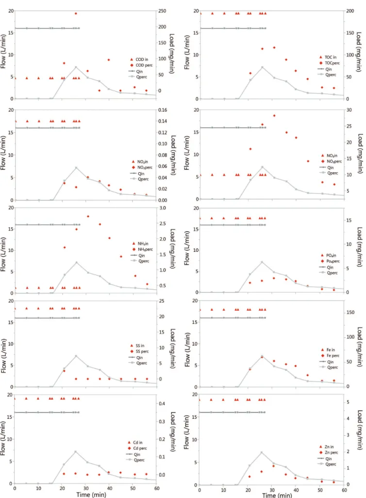
The study in the ield also assessed the pollutant retention eficiency. Water quality samples were collected and analyzed for
the inlet (Min(t)), which represents the pollution in runoff and for the storage (MS(t)). There was no outlow during the experiment
and, consequently, samples of Mout(t) were not collected. Table 6 presents a summary of the pollutant mass balance
results, including pollutant removal eficiency for the stored water.
Despite the higher concentration values for the pollutants in the storage, the total load was low due to the low stored volume.
Therefore, we found good results in the removal eficiency, with
the lowest value of 87% for Cd. Regarding the stored water (MS(t)), most of the treatment process had already occurred, such
as absorption by plant tissues, soil sorption, iltration through the
sand and gravel layers and degradation. Therefore, the removal of some pollutants at this stage is common. In addition, water stored
over time will percolate with equal or better quality, as it will still
increase soil contact and longer reaction time (DAVIS et al., 2006). However, there was no data monitored for MI(t).
Macedo (2017) also carried out a different study monitoring real rainfall events in this same bioretention device applied
in the ield. For this study, the results indicated lower values of water retention eficiency (average of 68%) and pollutant removal eficiency (around 70% for all pollutants and exporting for nitrate). The difference in the eficiency values obtained can be explained by the variation in the rainfall intensity and total volume precipitated of the real events monitored, with the low
rate and control volume of the controlled event. The real event
ranged from an equivalent depth of 2.6 mm to 38 mm, while the
controlled event was only 0.43 mm. Therefore, the total volume
and load to be treated in this experiment were much lower than
for what occurred in real events.
Despite the limitations observed when comparing with real events, the results obtained by the controlled event enabled us to advance in some interpretations. Due to the low storage measured,
Table 5. Concentrated water balance. percolation rate and water retention eficiency for ield-scale event.
Total volume (m3) / Equivalent depth(mm) Percolation
rate (%)
Eff ret
hid. (%)
In Out Percolated Storage
Table 7. Comparison between the inlet volumes, net volumes and application rate on the laboratory and ield scales.
Scale Net storage
volume (m3) Inlet volume (m
3) Application rate
(in % of net volume)
Eff quanti
med (%)
Eff quali
med (%)
Laboratory 0.5 0.31 - 0.53 62.1 - 106.6 99.9 -17.0
Field 62.0 10.12 16.3 100.0 95.1
the importance of the percolation in the retention/detention process could be noted. Moreover, problems could be identiied in
the monitoring method for small volumes of the storage variable as the level sensor can measure only the volume converted in the
liquid depth in the piezometers.
Comparing the scales of analysis
After evaluating the water balance and mass balance results for the two analysis scales separately, it was important to make a comparative study by raising the limiting factors for a proper
comparison. In this study, the condition of equivalence between
the scales was made based on the parameters’ precipitation
equivalent to real events, low rate and duration, as described in the
methodology section. The two scales presented the same design
and coniguration, but without ensuring geometric, kinematic
and dynamic similarity.
At irst, the results obtained for the two scales, with the pre-established equivalence parameters, are presented discussing
the similarities and differences in the performance results of the
systems, listing the possible causes for the differences. Subsequently, care to be taken when extrapolating the results from different
scales, and recommendations for future comparative studies are presented.
Table 7 presents a comparison between the retention
capacities, input conditions, qualitative and quantitative eficiencies
obtained in both evaluation scales. The results indicate that the
total control volume and the low rate range in the scales were insuficient to completely saturate the iltering media, leading to
no outlow and, consequently, water retention eficiency of almost
100% in both cases.
For the bioretention box, a control volume greater than
the total storage capacity was applied, reaching a value of 106.6% for the application rate (ratio between the inlet volume and total
storage capacity), i.e. a volume exceeding up to 7%. However, storage in the iltering media achieved values around only 80% of
the total capacity. The other portion of volume was converted into percolation, even before the complete saturation of the media.
As for the ield scale, the results indicate negligible storage
and total percolated volume achieving almost the same value for the inlet volume. However, it was hypothesized that the water was
stored as moisture, not generating a liquid level, but still retaining the volume. Regarding the qualitative aspects of the runoff, before
and after treatment, the sampling points in the two scales were different. For the laboratory scale, the samples were collected from
the percolation outlet, while for the ield scale, the samples were
collected from the visit pipes. Despite this difference in sampling,
both scales can be compared for treatment eficiency as the stored water will percolate at some point, with an equal or high quality
since it will still increase soil contact and with a longer reaction time (DAVIS et al., 2006).
Higher removal rates were found for the device in the ield,
indicating better treatment than the laboratory scale. However, in the literature review, the studies found lower rates of pollutant removal in real-scale applications. The application rate and Hequivalent
explain the difference in the results found in this paper and in the literature. Although the low rate was the same for the two scales to ensure equivalence, the application rate for the ield scale was at least 3x less than for the laboratory scale. Proportionally, for the bioretention device in the ield, the volume to be treated in the same unit of iltering media is lower, leading to a greater treatment.
Moreover, we also compared parameter Hequivalent for both
scales. This parameter represents the height value equivalent to the real bioretention zone responsible for the qualitative treatment, so
that the treatment capacities for devices with different scales and
conigurations could be compared. Its calculation is made by the
ratio between the net volume and surface area (shown in Table 1). For this study, Hequivalent is higher for the ield scale than for the laboratory scale, with values of 1.02 m and 0.32 m, respectively.
This means, even at equal application rates in both scenarios, the ield scale will still have greater Hequivalent due to its dimensions, corroborating a better treatment.
The bottom permeability also differs between the two
scales, which also inluences the performances. The laboratory
scale bioretention presents a hollow bottom for the percolated
volume collection, not presenting the same dificulty to the low as the soil generates in the ield.
Comparing the results for the two scales, we noticed that
even with a hydraulic equivalence through an average low rate is insuficient to ensure a similarity in the results. For a proper
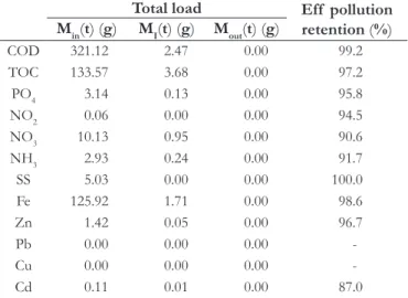
Table 6. Mass balance and pollutant removal eficiency for ield
scale. These are the results for the controlled event with Fm of
52 cm/h, six samples for Min(t) and three for MS(t).
Total load Eff pollution retention (%)
Min(t)(g) MI(t)(g) Mout(t)(g)
COD 321.12 2.47 0.00 99.2
TOC 133.57 3.68 0.00 97.2
PO4 3.14 0.13 0.00 95.8
NO2 0.06 0.00 0.00 94.5
NO3 10.13 0.95 0.00 90.6
NH3 2.93 0.24 0.00 91.7
SS 5.03 0.00 0.00 100.0
Fe 125.92 1.71 0.00 98.6
Zn 1.42 0.05 0.00 96.7
Pb 0.00 0.00 0.00
-Cu 0.00 0.00 0.00
extrapolation of the experiment’s results and data in different
scales, a study of the dimensional analysis should be carried out, ensuring physical similarity between them. Thus, the geometric
similarity should be ensured – with a constant scale factor and equal roughness; kinematic similarity - so that the time intervals
used are the same; and dynamic similarity - ensuring dimensionless
groups with equal value. Given the physical similarity, it is known
that the hydraulic and treatment processes occurring within the devices in the two different scales will be the same.
However, it is known that it is not always possible to ensure a physical similarity between the scales, since the great advantage of
the laboratory application is the reduced size, lexibility of layouts
and testing new conditions to identify key-factors. Therefore, we present the essential parameters that should be similar for the comparisons and that should be taken into account in the discussion
of the results for different scales, mainly in the laboratory and ield:
(1) Equivalent low rate – Even though it is an important parameter, it can be observed that it does not ensure similarity in the results by itself. (2) Control volume: the control volume should be established in such a way that the same application rate is applied in both scales. (3) Equivalent net depth (Hequivalent): For analysis of the qualitative results, the Hequivalents of the experimental devices should be close to each other in order to present similar treatment capabilities.
In addition, variations in data acquisition methods can
generate undesirable differences in the results, not necessarily related to differences in the scales. In this study, we observed that the
different methods for storage acquisition led to misinterpretations regarding the dynamics of bioretention in the ield.
CONCLUSION
From the monitoring of the controlled events, it was
possible to obtain eficiency values for the qualitative treatment per pollutant and an average value of water retention eficiency.
It is important to remember that these results were obtained for
low rates ranging from 47.5 cm / h to 183.9 cm / h, in relation to the surface area of the two experimental devices:
• For the laboratory scale, we found a water retention
eficiency of 99.9% and percolation rates ranging from
32% to 76%. Even if the sand layer was not completely saturated, the percolation process occurred. This result indicates the importance of considering the percolation in the retention and detention capacity of bioretention
practices. The qualitative analysis demonstrates low pollutant removal eficiency and export for NO3 and NH3. These results are also observed in other studies;
• For the ield scale, when comparing with other
non-controlled experiments in the same bioretention, the values for water retention and pollutant removal are signiicantly higher, indicating a low rate that corresponds only to
small precipitation events. However, these results help to identify the importance of the percolation process in the
retention/detention process and problems in quantifying
the storage only by the piezometers.
Comparing the two scales of analysis, we identiied the main
parameters that affect the results for the different scales, which are: the flow rate, the control volume/application rate and the equivalent net depth. For a suitable comparison, these values should be as close as
possible between the laboratory-scale and ield-scale experimental
devices. However, aware of the limitation of laboratory devices
and also that the lexibility of layouts is one of its advantages,
if these parameters are not similar, they should be observed and taken into account when analyzing the results.
For the experimental devices analyzed in this study, further trials will be required to test a wider range of control volumes and low rates, which will be able to completely ill the device net volume. On a ield scale, methods to measure the sand humidity
should be included in order to better analyze the storage, even for small volumes.
ACKNOWLEDGEMENTS
CAPES 88887.091743/2014-01 (ProAlertas CEPED/USP), CNPq 465501/2014-1 and FAPESP 2014/50848-9 INCT-II (Climate Change, Water Security), CNPq PQ 312056/2016-8 (EESC-USPCEMADEN/MCTIC) and CAPES PROEX (PPGSHS EESC USP), FAPESP 2015/20979-7 Optimization of operation
and maintenance of LID practices in subtropical climate.
REFERENCES
AMERICAN PUBLIC HEALTH ASSOCIATION – APHA.
Standard method for water and wastewater examination. 17th ed.
Washington: APHA, 1992.
BAPTISTA, M. B.; NASCIMENTO, N. O.; BARRAUD, S. Técnicas compensatórias em drenagem urbana. Porto Alegre: ABRH, 2005. 266 p.
BRATIERES, K.; FLETCHER, T. D.; DELETIC, A.; ZINGER, Y. Nutrient and sediment removal by stormwater biofilters: a large-scale design optimisation study. Water Research, v. 42, n. 14, p. 3930-3940, 2008. PMid:18710778. http://dx.doi.org/10.1016/j. watres.2008.06.009.
BROWN, R. A.; HUNT, W. F. Improving bioretention/biofiltration performance with restorative maintenance. Water Science and Technology, v. 65, n. 2, p. 361-367, 2012. PMid:22233916. http://
dx.doi.org/10.2166/wst.2012.860.
CHAHAL, M. K.; SHI, Z.; FLURY, M. Nutrient leaching and copper speciation in compost-amended bioretention systems. The Science of the Total Environment, v. 556, p. 302-309, 2016. PMid:26977536.
http://dx.doi.org/10.1016/j.scitotenv.2016.02.125.
DAVIS, A. P. Field performance of bioretention: water quality. Environmental Engineering Science, v. 24, n. 8, p. 1048-1064, 2007.
http://dx.doi.org/10.1089/ees.2006.0190.
DAVIS, A. P.; SHOKOUHIAN, M.; SHARMA, H.; MINAMI,
C. Water quality improvement through bioretention media:
v. 78, n. 3, p. 284-293, 2006. PMid:16629269. http://dx.doi.
org/10.2175/106143005X94376.
ERICKSON, A. J.; WEISS, P. T.; GULLIVER, J. S. Optimizing stormwater treatment practices: a handbook of assessment and maintenance. New York; Springer, 2013. http://dx.doi.org/10.1007/978-1-4614-4624-8.
FLETCHER, T. D.; ANDRIEU, H.; HAMEL, P. Understanding, management and modelling of urban hydrology and its
consequences for receiving waters: a state of the art. Advances in Water Resources, v. 51, p. 261-279, 2013. http://dx.doi.org/10.1016/j. advwatres.2012.09.001.
GUTIERREZ, L. A. R. Avaliação da qualidade da água de chuva e de um sistema iltro-vala-trincheira de iniltração no tratamento do escoamento supericial direto predial em escala real em São Carlos - SP. 2011. 198 f.
Dissertação (Mestrado em Engenharia Urbana) – Universidade
Federal de São Carlos, São Carlos, 2011.
HATT, B.; FLETCHER, T.; DELETIC, A. Hydrologic and pollutant removal performance of stormwater biofiltration systems at the field scale. Journal of Hydrology, v. 365, n. 3-4, p. 310-321, 2009.
http://dx.doi.org/10.1016/j.jhydrol.2008.12.001.
HSIEH, C. H.; DAVIS, A. P. Evaluation and optimization of bioretention media for treatment of urban storm water runoff. Journal of Environmental Engineering, v. 131, n. 11, p. 1521-1531, 2005.
http://dx.doi.org/10.1061/(ASCE)0733-9372(2005)131:11(1521).
HSIEH, C. H.; DAVIS, A. P.; NEEDELMAN, B. A. Nitrogen removal from urban stormwater runoff through layered bioretention columns. Water Environment Research, v. 79, n. 12, p. 2404-2411, 2007. PMid:18044357. http://dx.doi.org/10.2175/106143007X183844.
LAURENSON, G.; LAURENSON, S.; BOLAN, N.; BEECHAN, S.; CLARK, I. The role of bioretention systems in the treatment of stormwater. In: SPARK, D. L. (Ed.). Advances in agrononmy. Philadelphia: Elsevier, 2013.
LI, H.; DAVIS, A. P. Urban particle capture in bioretention media. I: Laboratory and field studies. Journal of Environmental Engineering, v. 134, n. 6, p. 409-418, 2008. http://dx.doi.org/10.1061/ (ASCE)0733-9372(2008)134:6(409).
LIU, J.; SAMPLE, D. J.; OWEN, J. S.; LI, J.; EVANYLO, G. Assessment of selected bioretention blends for nutrient retention
using mesocosm experiments. Journal of Environmental Quality, v. 43, n. 5, p. 1754-1763, 2014. PMid:25603260. http://dx.doi.
org/10.2134/jeq2014.01.0017.
LUCAS, A. H. Monitoramento e modelagem de um sistema iltro-vala-trincheira de iniltração em escala real. 2011. 159 f. Tese (Doutorado) - Universidade Federal de São Carlos, São Carlos, 2011.
LUCAS, A. H.; SOBRINHA, L. A.; MORUZZI, R. B.; BARBASSA,
A. P. Avaliação da construção e operação de técnicas compensatórias
de drenagem urbana: o transporte de finos, a capacidade de
infiltração, a taxa de infiltração real do solo e a permeabilidade da manta geotêxtil. Engenharia Sanitaria e Ambiental, v. 20, n. 1, p. 17-28, 2015. http://dx.doi.org/10.1590/S1413-41522015020000079923.
LUCKE, T.; NICHOLS, P. W. B. The pollution removal and stormwater reduction performance of street-side bioretention basins after ten years in operation. The Science of the Total Environment, v. 536, p. 784-792, 2015. PMid:26254078. http://dx.doi.org/10.1016/j. scitotenv.2015.07.142.
MACEDO, M. B. Optimizing low impact development (LID) practices in subtropical climate. 2017. 89 f. Dissertação (Mestrado em Hidráulica e Saneamento) – Escola de Engenharia de São Carlos, Universidade
de São Paulo, São Carlos, 2017.
MAGLIONICO, M. Indagine sperimentale e simulazione numerica degli aspetti qualitativi dei delussi nelle reti di drenaggio urbano. 1998. 217 f. Tese (Doutorado) - Università di Bologna, Bologna, 1998.
MANGANGKA, I. R.; LIU, A.; EGODAWATTA, O.; GOONETILLEKE, A. Performance characterisation of a stormwater treatment bioretention basin. Journal of Environmental Management, v. 150, p. 173-178, 2015. PMid:25490107. http://
dx.doi.org/10.1016/j.jenvman.2014.11.007.
MARENGO, J. A.; SCHAEFFER, R.; ZEE, D.; PINTO, H. S. Mudanças climáticas e eventos extremos no Brasil. Rio de Janeiro:
FBDS, 2010. Available from: <http://www.fbds.org.br/cop15/
FBDS_MudancasClimaticas.pdf >. Access on: 1 oct. 2010.
MARSALEK, J.; SCHREIER, H. Innovation in stormwater management in canada: the way forward. Water Quality Resources, v. 44, n. 1, p. 5-10, 2009.
PETTERSON, S. R.; MITCHELL, V. G.; DAVIES, C. M.; O’CONNOR, J.; KAUCNER, C.; ROSER, D.; ASHBOLT, N. Evaluation of three full-scale stormwater treatment systems with respect to water yield, pathogen removal efficacy and human health risk from faecal pathogens. The Science of the Total Environment, v. 543, n. Pt A, p. 691-702, 2016. PMid:26615487. http://dx.doi.
org/10.1016/j.scitotenv.2015.11.056.
ROSA, A. Bioretention for diffuse pollution control in SUDS using experimental-adaptative approaches of ecohydrology. 2016. 109 f. Tese
(Doutorado em Hidráulica e Saneamento) - Escola de Engenharia
de São Carlos, Universidade de São Paulo, São Carlos, 2016.
RYCEWICZ-BORECKI, M.; MCLEAN, J. E.; DUPONT, R. R. Nitrogen and phosphorus mass balance, retention and uptake in
six plant species grown in stormwater bioretention microcosms.
Ecological Engineering, v. 99, p. 409-416, 2017. http://dx.doi.
org/10.1016/j.ecoleng.2016.11.020.
URBONAS, B.; STAHRE, P. Stormwater: best management practices and detention for water quality, drainage, and CSO management. New Jersey: PTR PH, 1993.
VALVERDE, M. C.; MARENGO, J. A. Mudanças na circulação
atmosférica sobre a América do Sul para cenários futuros de clima projetados pelos modelos globais do IPCC AR4. Revista Brasileira de Meteorologia, v. 25, n. 1, p. 125-145, 2010. http://dx.doi.
org/10.1590/S0102-77862010000100011.
WANG, J.; ZHANG, P.; YANG, L.; HUANG, T. Adsorption characteristics of construction waste for heavy metals from urban stormwater runoff. Chinese Journal of Chemical Engineering, v. 23, n. 9, p. 1542-1550, 2015. http://dx.doi.org/10.1016/j.cjche.2015.06.009.
WANG, J.; ZHANG, P.; YANG, L.; HUANG, T. Cadmium removal from urban stormwater runoff via bioretention technology and effluent risk assessment for discharge to surface water. Journal of Contaminant Hydrology, v. 185-186, p. 42-50, 2016. PMid:26826541.
http://dx.doi.org/10.1016/j.jconhyd.2016.01.002.
WINSTON, R. J.; LUELL, S. K.; HUNT, W. F. Evaluation of undersized bioretention for treatment of highway bridge deck runoff. In: INTERNATIONAL CONFERENCE ON URBAN DRAINAGE, 12., 2011, Porto Alegre, Brazil. Proceedings... Porto
Alegre: IWA, 2011.
YOUNG, C. E. F.; AGUIAR, C.; SOUZA, E. Valorando Tempestades:
custo econômico dos eventos climáticos extremos no Brasil nos
anos de 2002-2012. São Paulo: Observatório do Clima, 2015.
ZHANG, L.; SEAGREN, E. A.; DAVIS, A. P.; KARNS, J. S. Effects of temperature on bacterial transport and destruction in bioretention media: field and laboratory evaluations. Water Environment Research, v. 84, n. 6, p. 485-496, 2012. PMid:22866389.
http://dx.doi.org/10.2175/106143012X13280358613589.
Authors contributions
Marina Batalini de Macedo: Contributed to the collection and
laboratory analysis of quantity and quality samples in the laboratory and in the ield, in the data analysis and treatment of water and
pollutant load balances, in the discussion and interpretation of the results and writing of the article.
César Ambrogi Ferreira do Lago: Contributed to the collection and laboratory analysis of quantity and quality samples in the laboratory and in the ield, in the data analysis and treatment of water and
pollutant load balances, in the discussion and interpretation of the results and writing of the article.
Eduardo Mario Mendiondo: Contributed to the construction of
the laboratory and ield models, in the discussion and interpretation
of the results and writing of the article.
Vladimir Caramori Borges de Souza: Contributed to the construction
of laboratory and ield models, in the data analysis and treatment