Abstract
In this manuscript, we solve an asymmetric 2D problem for a long cylinder. The surface is assumed to be traction free and subjected to an asymmetric temperature distribution. A direct approach is used to solve the problem in the Laplace transformed domain. A numerical method is used to invert the Laplace transforms. Graphically results are given and discussed.
Keywords
Fractional Calculus; Infinitely Long Cylinder; Thermoelasticity
2D Problem for a Long Cylinder in the Fractional
Theory of Thermoelasticity
NOMENCLATURE
t time
T absolute temperature
ij Stress tensor components
density
, Lamé's constants
= (3+2) t
αt coefficient of linear thermal expansion k thermal conductivity
0
T
reference temperature assumed to be such that (T T0) /T0 1,
0 constants such that
0> 0, 0 ≤≤ 1cE
specific heat per unit mass in the absence of deformationHany H. Sherief a W. E. Raslan b
aDepartment of Mathematics,
Alexan-dria University, AlexanAlexan-dria, Egypt . [email protected]
bDepartment of Mathematics and
engi-neering physics, Mansoura University, Mansoura, Egypt . [email protected]
http://dx.doi.org/10.1590/1679-78252431
1 INTRODUCTION
In 1967 Lord and Shulman (Lord & Shulman, 1967) were the first to generalize Biot’s theory of coupled thermoelasticity. This theory ensures finite speeds of propagation for waves. Sharma and Pathania studied wave propagation (Sharma & Pathania, 2006), Sherief and Anwer solved a two dimensional problem for an infinitly long cylinder (Sherief & Anwar, 1994) , Sherief and Ezzat obtained the fundemental solution in the form of series of functions (Sherief & Ezzat, 1994) and Sherief and Saleh solved a generilized thermoelastic problem for an infinite body with a spherical cavity using complex countor integration (Sherief & Saleh, 1998).
An ingoing process is the use of fractional calculus to create a replacement for many physical models (Hilfer et al., 2000; Machado, Galhano, & Trujillo, 2013). Sherief et al used fractional deriva-tive to generalized Hodgkin and Huxley model (Sherief, El-Sayed, Behiry, & Raslan, 2012). Povstenko used fractional derivatives to derive new models for the conduction of heat (Povstenko, 2009).
The fractional theory of thermoelasticity was introduced in 2010 (H. H. Sherief, El-Sayed, & Abd El-Latief, 2010). The main reason behind the introduction of this theory is that it predicts retarded response to physical effects, as is found in nature, as opposed to instantaneous response predicted by the generalized theory of thermoelasticity. This retarded response stems from the fact that fractional derivatives are in fact integrals over time. Physically this results from the weak van der Walles forces. In the following, some applications of the fractional order theory of thermoelasticity are intro-duced. Raslan has solved a problem for a cylindrical cavity (Raslan, 2014). El-Karamany and Ezzat applied fractional order theory to perfect conducting thermoelastic medium (El-Karamany & Ezzat, 2011; Ezzat & El-Karamany, 2011), Sherief and Abd El-Latief studied the effect of variable thermal conductivity on a half-space under the fractional order theory of thermoelasticity (Sherief & Abd El-Latief, 2013) , also they applied the theory to a 1D problem for a half‐space (Sherief & Abd El‐ Latief, 2014) , Tiwari and Mukhopadhyay introduced Boundary Integral Equations Formulation for Fractional Order Thermoelasticity ( Tiwari & Mukhopadhyay, 2014).
2 FORMULATION OF THE PROBLEM
In this manuscript, we consider a homogeneous isotropic cylinder of radius “
a
” and infinite length. We shall use the cylindrical coordinates (r,,z). The initial conditions are taken to be homogeneous.The surface of the cylinder is assumed to be traction free and subjected to an asymmetric temperature distribution.
The physics of the medium under discussion ensures that all quantities are independent of z. all functions depend on r and . The displacement vector has the non-zero components u and v in r and directions, respectively. The governing equations are
22
2
graddiv gradT t
u
u u (1)
1 2
0 1 E 0
k T c T T e
t t
where 2 2 2 2 1 1 r
r r r r
Applying the divergence operator to both sides of equation (1), we obtain
2 2 22
2 e T e
t
(3)
where e is the cubical dilatation given by
1 1
div v
e ru
r r r
u (4)
The constitutive equations can be written as
0
2rr
u
e T T
r
(5a)
0
2 v
u e T T
r
(5b)
0
zz
e
T
T
(5c)1
r
v v u
r r r
(5d)
0
rz z
(5e)We shall use the following non-dimensional quantities
2 0 2 0 0 , , , , , , 2 ij ijr c r u c u t c t v c v
T T
τ c τ
where c 2 , ρcE
ρ k
.
These non-dimensional variables were first introduced by Sherief (1980) in his PhD thesis. They were obtained by trial and error. They are useful because the solution obtained using these variables does not depend on the units used.
Using the above non-dimensional quantities, (dropping the asterisk for convenience), the govern-ing equations take the form
22 2 2 2
2
1 grade grad
where 2 2
. Equation (6) gives the following two equations
2 2 2
2 2 2
2 2 2 2
1 rv 1
e u u
r r r r r t
(7)
22 2 2
2
1 rv 1
e u v
r r r
r r r r r t
(8)
2 2 2 2 e e t
(9)
1 20 1 e
t t
(10)
2
22 2 rr u e r
(11a)
2
22 v 2
u e r
(11b)
22
2zz
e
(11c)1
r
v v u
r r r
(11d)
0
rz z
(11e)where T0 2 / (2 ) k.
We note that in the above transformed equations, all the variables and constants (
, , 0
) are non dimensional.The fractional derivative used in equation (10) is the Caputo derivative. The boundary conditions can be expressed as:
, ,
0
rr
a
t
(12a)
, ,
0r a t
(12b)
a
, ,
t
f
,
t
(12c)affecting the boundary so the normal component of stress that act to neutralize these forces are also zero. The stress component
is the resultant of internal forces and not necessarily zero.3 SOLUTION IN THE TRANSFORM DOMAIN
Applying the Laplace transform with parameter s (denoted by an over bar) to both sides of equations
(7), (9-11), we get the following equations
2 2 2
2 2 2
2 2 2 2
1 rv 1
e u u
r r r r r t
(13)
2
2s
2e
(14)
2 1
1
0 0
s
s
s
s
e
(15)
2
22 2
rr u e
r
(16a)
2
22 v 2
u e
r
(16b)
22
2zz
e
(16c)1
r v v u
r r r
(16d)
Equations (12) transform to:
, ,
0rr a s
(17a)
, ,
0r a s
(17b)
a, ,s
f
,s
(17c)Applying the operator ( 2 s2)to both sides of equation (15) and multiplying both sides of equation (14) by
s0s1
and subtracting, we obtain
2 1 3
0 0
(1 )( ) (1 ) 0
4 s
s τ s 2 s τ s
(18)
Equation (18) can be written in the form:
0
)
(
)
where k12andk22 are the complex roots which have positive real parts of the following characteristic equation
4 2 2 1 3
0 0
(1 )(
)
(1
) 0
k
k
s
s
τ
s
s
τ
s
(20)The solution of equation (19) can be written in the form
2 1 i i
(21)where iis the solution of
2 2
0i i k
, i = 1, 2. (22a)
or 1 r i 12 2 2i ki2 i 0
r r r r
(22b)
The solution of equation (19), bounded at the origin, may be written as
2
2 2
0 1
( ) cos
in i n i
n i
A s k s I k r n
(23)where Ainare some parameters depends on s only and In(k ri ) is the modified Bessel function of
first kind of order n. In a similar manner, the solution for e compatible with equation (14) can be
written as
2
2
0 1
( ) cos
in i n i
n i
e A s k I k r n
(24)The Laplace transforms of equations (4) and (7) can be combined to give
2 2 2s
ru r 2
2 1
e 2er
(25)
Substituting from (23) and (24) into (25), we obtain
2 2 2
2 1
2 2 2
2 2 2
0 1 2 1 cos
i n i i
in
n i i n i
k s rk I k r
s ru A s n
n k n s I k r
(26)( ) ( ) ( ) and 1( ) ( ) 1 ( )
1 1
dIm x m dIm x m
Im x Im x Im x Im x
dx x dx x
(27)
After some manipulations, the solution of equation (26) takes the form
2 1 0 1 1 cos cos n iin i n i
n i
n n
n
nI k r
u A s k I k r n
r
B s I sr n r
(28)where Bn
s are some parameters depending on s only. We note that we have set B0 = 0 because0 0
( )
lim
r
I s r r
is not bounded.
Substituting from equations (24) and (28) into (3), and integrating with respect to
, we obtain
2
1
0 1
1 sin
in n i n n n
n i
n s
v A s I k r B s I sr I sr n
r r n
(29)We expand the function f
,s in a Fourier cosine series in
as
0
, n( )cos( )
n
f
s F s n
where
F
n
s
are the Fourier coefficient given by
0
0
1 ,
F s f s d
02 , cos
n
F s f s n d
We have chosen to expand the function in a cosine series to facilitate the computations. This means that we take the temperature as an even function of
. A full expansion in terms of sine and cosine will add nothing to the physical meaning of the problem considered.Substituting from equations (23), (24), and (28) into Equation (16a), and applying the boundary condition (17a), we get for n = 0
2
2 2
0 1 0
1
2 i 0
i i i
i
k
s I k a I k a A s
a
(30)
2
2 2 2
1 1 1 1 1 2 1 0
n i i n i in
i
n n n
s a n n I k a k aI k a A s
n I sa saI sa B s
(31)Similarly, boundary equation (17b) yields for n = 1,2,3,…
2 1 12 2 2
1 1
1 0
2
n i i n i in i
n n n
n I k a k aI k a nA s
s a sa
n I sa I sa B s
n n
(32)Finally the boundary condition (17c) leads to for n = 0
2
2 2
0 0 0
1
( )
i i i
i
A s k s I k a F s
(33)and for n = 1,2,3,…
2
2 2
1
( )
in i n i n
i
A s k s I k a F s
(34)Equations (30) and (33) can be solved to obtainA10andA20,
2 2
0 0 2 1 2 2
10 F a( I k a s - 2I k a k )
A
2
20 1 1 1 0 1
20 F (2I k a k -a I k a s )
A
where
2 2 2 2 2 2
0 1 0 2 1 2 0 1 1 2 2 1
2 2
0 2 1 1 1 2
( ( - )- 2( ( - )
( - )))
a I k a I k a s k k I k a I k a k k s
I k a I k a k s k
Equations (31), (32) and (34), can be written as:
11 1n 12 2n 13 n 0
a A a A a B
21 1n 22 2n 23 n 0
a A a A a B
31 1n 32 2n n
a A a A F
2 2 211 12 1 n 1 1 n 1 1
a
s a n n I k a k aI k a
2 2 2
12 12 1 n 2 2 n 1 2
a
s a n n I k a k aI k a
13
1
n n 1a
n
I
sa
saI
sa
21
1
n 1 1 n 1 1a
n n
I
k a
nk aI
k a
22
1
n 2 2 n 1 2a
n n
I
k a
nk aI
k a
2 2 2
23 1 2 n n 1
s a sa
a n I sa I sa
n n
2 2
31 1 n
(
1)
a
k
s
I
k a
2 2
32 2 n
(
2)
a
k
s
I
k a
Solving the above equations, we obtain
12 23 13 22
1n n
a a a a F
A
13 21 11 23
2n n
a a a a F
A
13 21 11 23
n
a a a a
B
where
a
23 12 31 11 32
a a
a a
a
13 21 32
a a
a a
22 31
4 NUMERICAL RESULTS AND DISCUSSION
We shall apply our results to a medium composed of the copper material. The parameters of the problem are k = 386 W/(m K), t = 1.78 (10)-5 K-1, cE = 381 J/(kg K), = 8886.73, = 3.86 (10)10
kg/(m s2), = 7.76 (10)10 kg/(m s2), = 8954 kg/m3, T0 = 293 K,
0
/12
, a = 1 m, 0 = 0.025s and = 0.0168.
The above values were obtained from ((Thomas, 1980) except for 0 which was assumed.
We shall consider two cases of the applies heating
Case 1
, 0 00 otherwise
t or
f
t
,
Fn are thus given by
00 2 and n 2 sin 0 1 1n
F F n
n
Case 2
, 0 ,0 otherwise t
f
t
The Fourier coefficients Fn are thus given by
2
0 0 0
0
0 2 , n 2 sin cos 2 12
n n
F F
n n n
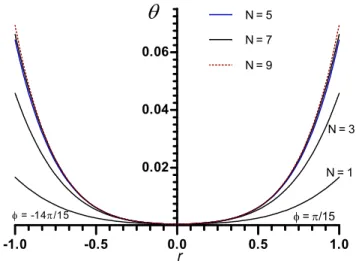
Two methods were tried to solve the problem. Firstly, the Laplace transform of the terms of the series were inverted term by term and then summed up as a series of real numbers. Secondly, the series was summed up as a complex-term series and then the inverse Laplace transform was applied. It was found that the first method is better. It achieves higher order of convergence. Figure (1) shows the solution for different values of N (maximum number of terms taken in the series). It was found
that the solution stabilized after N = 9.The programming was done using the Fortran language on
an I7 core computer. The numerical inversion of the Laplace transform was done using a method outlined in (Honig & Hirdes, 1984).
Figure 1: Convergente graph for temperatura at = 0.5 (case 1) for t = 0.1
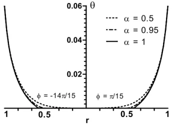
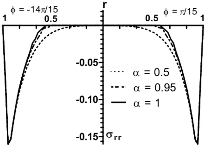
Figs 2 to 5 represent case 1 while figures 6 to 9 represent case 2. We did the evaluations using 3 values of , which are: = 0.5, 0.95 and 1 for t = 0.06.
The results are shown in Fig. 2, 6 for the temperature distribution, Fig. 3, 7 for the radial dis-placement distribution, Fig. 4, 8 for the tangential disdis-placement distribution and Fig. 5, 9 For stress distribution.
-1.0 -0.5 0.0 0.5 1.0
0.02 0.04 0.06
=/15
= -14/15
N = 1 N = 3 N = 9
N = 5 N = 7
Figure 2: Temperature distribution for different (case 1) for t = 0.06
Figure 3: Radial displacement distribution for different (case 1) for t = 0.06
Figure 4: Tangential displacement distribution for different (case 1) for t = 0.06
0.02 0.04 0.06
= 0.5
= 0.95
= 1
=/15
= -14/15
1
1
0.5
r
0.5
= 0.5
= 0.95
= 1
u
*(10)
-3 = /15
= -14/1 5
1 0.5 0.5 1
0.5 1.5
1
r
= 0.5
= 0.95
= 1 v*(10)-4
=/15
= -14/15
1 0.5 0.5 1
0.5 1.5
1 2
Figure 5: Radial stress distribution for different (case 1) for t = 0.06
Figure 6: Temperature distribution for different (case 2) for t = 0.06
Figure 7: Radial displacement distribution for different (case 2) for t = 0.06 -0.15
-0.10 -0.05
= 0.5
= 0.95
= 1
rr =/15
= -14/15
1
1 0.5
r
0.50.005 0.010
= .5
= .95
= 1
=/1 5
= -1 4/15
1
1 0.5 0.5
r
= .5
= .95
= 1 u*(10)-4
= /15
= -14/15
1 0.5 0.5 1
1 3
2
Figure 8: Tangential displacement for different (case 2) for t = 0.06
Figure 9: Radial stress distribution for different (case 2) for t = 0.06
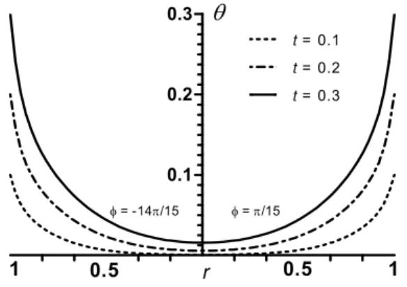
Figs 10 to 17 represent the time evolution of the different functions when t = 0.1, 0.2 and 0.3 for
= 0.5. Case 1 is shown in figures 10 to 13 while figures 14 to 17 represent case 2.
Figure 10: Temperature distribution for different t (case 1) for = 0.5
= .5
= .95
= 1 v*(10)-5
=/15
= -14/15
1 0.5 0.5 1
1.5
0.5 1 2
r
-0.020 -0.015 -0.010 -0.005
= .5
= .95
= 1
rr =/15
= -14/15
1
1 0.5 r 0.5
0.1 0.2 0.3
t = 0.1 t= 0.2 t = 0.3
=/15
= -14/15
1
Figure 11: Radial displacement distribution for different t (case 1) for = 0.5
Figure 12: Tangential distribution for different t (case 1) for = 0.5
Figure 13: Radial stress distribution for different t (case 1) for = 0.5
t = 0.1 t = 0.2 t = 0.3
u*(10)-2
=/15
= -14/15
1 0.5 0.5 1
1 2
r
t = 0.1 t = 0.2 t = 0.3
v*(10)-4
=/15
= -14/15
1 0.5 0.5 1
0.5 1.5
1 2
r
-0.4 -0.2
t = 0.1 t = 0.2 t = 0.3
rr
=/15
= -14/15
1
1 0.5 0.5
Figure 14: Temperature distribution for different t (case 2) for = 0.5
Figure 15: Radial displacement distribution for different t (case 2) for = 0.5
Figure 16: Tangential distribution for different t (case 2) for = 0.5
0.02 0.04
0.06 t = 0.1
t = 0.2 t = 0.3
=/15
= -14/15 1
1 0.5 0.5
r
t = 0.1 t = 0.2 t = 0.3
u*(10)-3
=/15
= -14/15
1 0.5 0.5 1
1 2
-1 3 4
t = 0.1 t = 0.2 t = 0.3
v*(10)-4
=/15
= -14/15
1 0.5 0.5 1
6
2 4
Figure 17: Radial stress distribution for different t (case 2) for = 0.5
Figures 18 and 19 represent temperature versus for case 1 and 2 respectively at t = 0.1 and r
= 0.4.
All these figures represent the functions as functions of r on the diagonal
/15
and14 / 15
.
Figure 18: Temperature vs
for different (case 1) for t = 0.1, r = 0.4-0.06 -0.04 -0.02 t = 0.1
t = 0.2 t = 0.3
rr =/15 = -14/15 1
1 0.5 r 0.5
-2 0 2
= 0.5 = 0.95
= 1
*(10)-3
2
1 4
Figure 19: Temperature vs
for different (case 2) at t = 0.1, r = 0.4The computations show that:
1. For α = 0.5, we can see from the graphs that the waves in the medium propagate with infinite speeds like the coupled theory of thermoelasticity. The program was run with α = 0 (correspond-ing to the coupled theory of thermoelaciticity), the results were almost identical to those when α = 0.5. For α = 1, the solution exhibits finite speeds since it is that of the generalized theory. The heat Equation associated with the couple theory of thermoelasticity ( = 0) is of parabolic type and predicts infinite speed of propagation for heat waves. The solution is nonzero (though it may be very small) at points far removed from the source of heating. The heat equation of the generalized theory of thermoelasticity ( = 1) is of hyperbolic type and predicts finite speed for heat waves. This means that heat propagates from the source of heating with a finite velocity. The solution is identically zero at points farther than the wave front. The location of the wave fronts and the value of the velocities for heat and elastic waves were discussed in (Sherief, H., & Hamza,1994).
2. For α
1, the situation is somewhat difficult to determine. The solution seems to travel with finite speeds. Of course, this is based on numerical evaluations only. This aspect would be very important when proved theoretically. The same conjecture was expressed in (Povstenko, 2011).References
Bell, W. Special Functions for Scientists and Engineers. 1968: D. Van Nostrand Company Ltd, London.
El-Karamany, A. S., & Ezzat, M. A. (2011). On fractional thermoelasticity. Mathematics and Mechanics of Solids, 16(3), 334-346.
Ezzat, M. A., & El-Karamany, A. S. (2011). Fractional order theory of a perfect conducting thermoelastic medium. Canadian Journal of Physics, 89(3), 311-318.
Hilfer, R., et al. (2000). Applications of fractional calculus in physics (Vol. 5): World Scientific.
-2 0 2
= .5
= .95
= 1
*(10)
-42 4 6
3
Honig, G., & Hirdes, U. (1984). A method for the numerical inversion of Laplace transforms. Journal of Computational and Applied Mathematics, 10(1), 113-132.
Lord, H. W., & Shulman, Y. (1967). A genergeeralized dynamical theory of thermoelasticity. Journal of the Mechanics and Physics of Solids, 15(5), 299-309.
Machado, J. T., Galhano, A. M., & Trujillo, J. J. (2013). Science metrics on fractional calculus development since 1966. Fractional Calculus and Applied Analysis, 16(2), 479-500.
Povstenko, Y. (2009). Thermoelasticity that uses fractional heat conduction equation. Journal of Mathematical Sci-ences, 162(2), 296-305.
Povstenko, Y. (2011). Fractional Cattaneo-type equations and generalized thermoelasticity. Journal of Thermal Stresses, 34(2), 97-114.
Raslan, W. (2014). Application of fractional order theory of thermoelasticity to a 1D problem for a cylindrical cavity. Archives of Mechanics, 66(4), 257-267.
Sharma, J., & Pathania, V. (2006). Thermoelastic waves in coated homogeneous anisotropic materials. International journal of mechanical sciences, 48(5), 526-535.
Sherief, H., & Abd El-Latief, A. (2013). Effect of variable thermal conductivity on a half-space under the fractional order theory of thermoelasticity. International Journal of Mechanical Sciences, 74, 185-189.
Sherief, H. H., & Abd El‐Latief, A. (2014). Application of fractional order theory of thermoelasticity to a 1D problem for a half‐space. ZAMM‐Journal of Applied Mathematics and Mechanics/Zeitschrift für Angewandte Mathematik und Mechanik, 94(6), 509-515.
Sherief, H. H., & Anwar, M. N. (1994). Two-dimensional generalized thermoelasticity problem for an infinitely long cylinder. Journal of thermal stresses, 17(2), 213-227.
Sherief, H. H., El-Sayed, A., & Abd El-Latief, A. (2010). Fractional order theory of thermoelasticity. International Journal of Solids and structures, 47(2), 269-275.
Sherief, H. H., El-Sayed, A., Behiry, S., & Raslan, W. (2012). Using Fractional Derivatives to Generalize the Hodgkin– Huxley Model Fractional Dynamics and Control (pp. 275-282): Springer.
Sherief, H. H., & Ezzat, M. A. (1994). Solution of the generalized problem of thermoelasticity in the form of series of functions. Journal of thermal stresses, 17(1), 75-95.
Sherief, H. H., & Hamza, F. A. (1994). Generalized thermoelastic problem of a thick plate under axisymmetric tem-perature distribution. Journal of thermal stresses, 17(3), 435-452
Sherief, H. H., & Saleh, H. A. (1998). A problem for an infinite thermoelastic body with a spherical cavity. International journal of engineering science, 36(4), 473-487.
Tiwari, R., & Mukhopadhyay, S. (2014). Boundary Integral Equations Formulation for Fractional Order Thermoelas-ticity. Computational Methods in Science and Technology, 20.