DAILY COUNTING OF MANUFACTURED UNITS SENT FOR QUALITY CONTROL: A BAYESIAN APPROACH
Jorge Alberto Achcar
1, Claudio Luis Piratelli
2*and Renata Regina Sandrim
3Received December 7, 2011 / Accepted December 15, 2012
ABSTRACT.This paper presents the statistical modeling for daily counting statistics of units that arrive for quality inspection at a food company. Different Poisson regression models were considered in order to analyze the data collected, with a Bayesian focus. The main objective was to forecast the daily average count based on co-variables such as days of the week. The analysis of co-variables is very often neglected by statistical packages that come with Discrete Event Simulation software. The discovery of the factors that influence these variations was essential to a more accurate modeling (the definition of simulation calendars) and enables industrial managers to make better decisions about the reallocation of people in the department, resulting in better planning of production capacity.
Keywords: poisson regression, Bayesian analysis, Markov Chain Monte Carlo methods.
1 INTRODUCTION
It is common to find a lot of variability in the daily counting of manufactured units in a produc-tion line. The statistical modeling of these data is useful as a diagnostic tool for the producproduc-tion systems (for example, for measuring the performance indicators by queue models), inference (forecasting) or simulation, especially for decisions on investment, production programming, allocation of the production capacity, and many other factors). Discovering these factors that affect variability may be of great interest to industrial engineers and industrial managers. In Queuing Theory (QT), counting analysis is essential in the choosing of the model appropriate to the queue object that is to be diagnosed – see, for example, Gross & Harris (1975), Kleinrock
*Corresponding author
1Professional Master Program in Production Engineering, University Center of Araraquara – UNIARA, Department of Social Medicine, FMRP, University of S˜ao Paulo, Brazil. E-mail: [email protected]
2Professional Master Program in Production Engineering, University Center of Araraquara – UNIARA, Brazil. E-mail: [email protected]
(1975), Larson & Odoni (1981). However, analytical queuing models have certain limitations to address complex problems (for example, the variability in counting due to the presence of covariates).
Discrete Event Simulation (DES) is used for either analyzing complex performance models or obtaining more detailed knowledge of a system – Kariet al.(1994). In DES, one of the analyst’s main objectives is to perform experiments on models that represent real systems, in order to predict future behavior – Kelton (2007). To this end, the identification of probability distributions for counting is crucial in order to have a reliable model of the reality that is to be shaped. DES approaches widely utilize random number generation in the analysis. Usually, the applied random distributions are quite simple but more complex distributions are required to get better accuracy in the model. Non-standard random distributions are required when the system cannot be modelled accurately using conventional probabilistic distributions. Efforts to deal with these situations are reported by Kariet al. (1994), Andrad´ottir & Bier (2000), Zhanget al. (2005), Leemis (2006), Yang & Liu (2012).
In industrial applications, Poisson distribution is common without considering co-variates. This modeling approach is commonly used by statistics packages which come with Discrete Event Simulation software. In general, these packages return a bad fit of data to the Poisson distribution, due to the high degree of variability in the counts (our case).
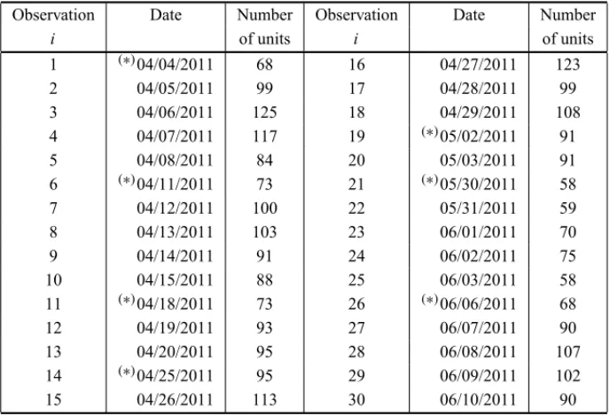
This paper considers the daily counting data for manufactured units sent for quality control at a food company in S˜ao Paulo State, Brazil, over a period of 30 non-consecutive days. This data set is presented in Table 1. Figure 1 shows the plot of the observed number of units (daily counting) against days, showing the high degree of variability for the daily counting.
Table 1– Daily counting data of manufactured units send to quality control.
Observation Date Number Observation Date Number
i of units i of units
1 (∗)04/04/2011 68 16 04/27/2011 123
2 04/05/2011 99 17 04/28/2011 99
3 04/06/2011 125 18 04/29/2011 108
4 04/07/2011 117 19 (∗)05/02/2011 91
5 04/08/2011 84 20 05/03/2011 91
6 (∗)04/11/2011 73 21 (∗)05/30/2011 58
7 04/12/2011 100 22 05/31/2011 59
8 04/13/2011 103 23 06/01/2011 70
9 04/14/2011 91 24 06/02/2011 75
10 04/15/2011 88 25 06/03/2011 58
11 (∗)04/18/2011 73 26 (∗)06/06/2011 68
12 04/19/2011 93 27 06/07/2011 90
13 04/20/2011 95 28 06/08/2011 107
14 (∗)04/25/2011 95 29 06/09/2011 102
15 04/26/2011 113 30 06/10/2011 90
30 25
20 15
10 5
0 130
120
110
100
90
80
70
60
50
Figure 1 – Daily counting (arrivals) versus days
Figure 1– Daily counting (arrivals) versus days.
This paper’s main objective is to analyze the daily counting data (arrivals at quality control) in Table 1 using Poisson regression models that assume certain co-variates, such as: days when the data was collected, and seasonality factors (specific days of the week). The focus is specifically on inference in the daily counting averageλ, depending on the co-variates, so that the schedules for the software simulation can reflect reality for the company. The inferences of interest were obtained using Bayesian methods. The posterior summaries of interest were obtained via Markov Chain Monte Carlo (MCMC) simulation methods, such as the popular Gibbs sampling algorithm (Gelfand & Smith, 1990) or the Metropolis-Hastings algorithm, when the conditional posterior distributions required for the Gibbs sampling algorithm do not have standard parametrical forms (see, for example, Chib & Greenberg, 1995).
Regression analysis of counting data has been studied by Hausmanet al. (1984), Zeger (1988), Blundellet al.(1995), Martz & Piccard (1995), Cameron & Trivedi (1998), Gurmuet al.(1999), Freeland & McCabe (2004a and b). Bayesian estimation has been proposed in count regression models by Harvey & Fernandes (1989), Albert (1992), Chibet al. (1998), Settimi & Smith (2000), Martz & Hamada (2003), McCabe & Martin (2005) and Zheng (2008).
According to Hsu & Wang (2007), modeling industry data sets is a challenge because: (1) a large sample of data is not always available; (2) there are some data items missing; (3) outliers interference; (4) the predictor variables are not correlated, among other reasons.
of standard existing Markov Chain Monte Carlo (MCMC) simulation methods. In this way, we do not need to use asymptotical results based on the asymptotical normality of the maximum likelihood estimators or standard asymptotical likelihood ratio tests which depend on large sam-ple sizes. These results could be a good justification for the use of Bayesian inference, espe-cially when the sample sizes are small or moderate, as is common in engineering applications (our case).
Bayesian methods have been used extensively in many applied areas, such as Business Admin-istration, Economy and Industrial Engineering. Some examples take from the Scielo scientific basis: Quinino & Bueno Neto (1997) used Bayesian methods to evaluate the accuracy of the qual-ity inspector; Pongo & Bueno Neto (1997) and Droguett & Mosleh (2006) proposed Bayesian inference to evaluate the reliability of products in development projects; Cavalcante & Almeida (2006) used multi-criteria method and Bayesian analysis to determine preventive maintenance in-tervals; Mouraet al.(2007) used the Bayesian methods to evaluate the efficiency of maintenance; Ferreiraet al.(2009) used the Bayesian approach in a portfolio selection problem; Barossi-Filho et al.(2010) used Bayesian analysis to estimate the volatility of financial time series, and Freitas et al.(2010) used the Bayesian approach to estimate the wearing out of train wheels.
The literature contains a rapidly growing number of published papers using the Bayesian para-digm in almost every applied area, such as medicine, economics, environmental sciences or engineering, since there has been a huge advance in computer hardware and software in the last twenty years. According to Fildes (2006), Bayesian methods have been gaining in prominence in the number of their citations in important journals in recent years and chief editors see them as a hot topic in forecasting (comprising counting problems). Armstrong & Fildes (2006) argue that many forecasting areas have developed methods, but few of them have been adopted in organizations in practice. Andrad ´ottir & Bier (2000) suggested the usage of Bayesian inference to estimate probability distributions parameters for input in simulation models. In this way, this paper gives a contribution for parameters estimation in a real count data from a food company (this approach can be used by Simulation analysts).
The paper is organized as follows: in Section 2 we present some Poisson regression models; in Section 3, we present a statistical analysis of the data presented in Table1; in Section 4, we present a discussion on the results obtained, and in Section 5 we present some concluding remarks.
2 STATISTICAL MODELING
LetYi be a random variable with a Poisson distribution given by,
P(Yi =yi)=
e−λiλyi
i
yi!
, (1)
Whereyi =0,1,2, . . .denotes the daily number of units (arrivals) for quality control in thei-th
In industrial applications it is common to use a Poisson distribution without considering co-variates. So, different Poisson regression models can be considered in analyzing the data set presented in Table 1, given as follows:
Model 1: Considerλigiven in (1), by
λi =exp(β0+β1Xi), (2)
where Xi denotes thei-th day(Xi =1,2, . . . ,30). In this case, it is assumed that days could
influence the daily counting of units sent to quality control. The formulation (2) guaranteesλito be positive, fori =1,2, . . . ,30.
Model 2: In this case, there is the addition of the quadratic termXi2in model (2), that is,
λi =exp(β0+β1Xi+β2Xi2), (3)
whereXi is defined in (2),i=1,2, . . . ,30.
Model 3: In this model, there is also anautoregressive effect of the daily counting yi−1in the modeling forλi, that is, a first order autoregressive model given by
λ1=exp(β0+β1X1), λi =exp(β0+β1Xi+β2yi−1),
(4)
where Xi is given in (2), and yi−1is the number of units (arrivals for quality control) on the (i−1)-th day,i =2,3, . . . ,30.
Model 4: Consider the introduction of another autoregressive term inλi, given by λ1=exp(β0+β1X1),
λ2=exp(β0+β1X2+β2y1), λi =exp(β0+β1Xi+β2yi−1+β3yi−2),
(5)
whereXi andyiare defined, respectively in (2) and (4), fori =3,4, . . . ,30.
Model 5 : Considerλi, in (1), given by
λ1=exp(β0+β1X1), λ2=exp(β0+β1X2+β2y1), λ3=exp(β0+β1X3+β2y2+β3y1), λi =exp(β0+β1Xi +β2yi−1+β3yi−2+β4yi−3)
(6)
wherei =4,5, . . . ,30.
our case, Mondays, where there seems to be a lower number of units sent to quality control as compared with other week days.
So, let us define the indicator variablezi =1 when thei-th day is a Monday andzi =0 when
thei-th day is not a Monday, fori=1,2, . . . ,30.
Assuming the models defined above, the likelihood function for the vector of parametersθ asso-ciated to each model is given by
L(θ )= 30
Y
i=1 e−λiλyi
i
yi!
(7)
whereθ =(β0, β1)for model 1;θ =(β0, β1, β2)for models 2 and 3;θ =(β0, β1, β2, β3)for model 4 andθ=(β0, β1, β2, β3, β4)for model 5.
For a Bayesian analysis, let us assume the following prior distributions for the regression param-etersβj of the models:
βj ∼N(aj;b2j) (8)
where N(aj;b2j)denotes a normal distribution with meanaj and varianceb2j, j =0,1,2,3,4.
Also prior independence is assumed among the models’ parameters.
Combining the joint prior distribution (a product of normal distributions) with the likelihood functionL(θ )given in (7), we obtain from the Bayes formula the joint posterior distribution for
θ(see for example, Box & Tiao, 1973).
The posterior summaries of interest are obtained using MCMC methods. Markov Chain Monte Carlo (MCMC) methods are a class of algorithms for sampling from probability distributions based on the construction of a Markov Chain that has the desired distribution as its equilibrium distribution (see for example, Paulinoet al., 2003). The state of the chain after a large number of steps is used as a sample of the desired distribution. The quality of the sample improves with the number of steps. Typical use of MCMC sampling can only approximate the target distribution, as there is always some residual effect from the starting position. The most common application of these algorithms is to numerically calculate multi-dimensional integrals. A special case is given by the Gibbs sampling algorithm, which is a special case of the Metropolis-Hastings algorithm (see Chib & Greenberg, 1995). Gibbs sampling uses the fact that given a multi-variate distri-bution it is simpler to sample from a conditional distridistri-bution than to marginalize by integrating over a joint distribution. Suppose we want to obtain samples ofX = {x1, . . . ,xn}from a joint
distribution p(x1, . . . ,xn). Denote thei-th sample byX(s) = {x(Is), . . . ,xss(s)}. We proceed as follows:
1. We begin with some initial valueX(0)for each variable.
2. For each samplei = {1. . .k}, sample each variablex(ji)from the conditional distribution p(x(ji)|x1(i), . . . ,x(j−i)1,x(j+i−11), . . . ,xn(i−1)). That is, sample each variable from the
The samples then approximate the joint distribution of all variables. Furthermore, the marginal distribution of any subset of variables can be approximated by simply examining the samples for that subset of variables, ignoring the rest. In addition, the expected value of any variable can be approximated by averaging over all the samples.
A great simplification in the simulation of samples for the joint posterior distribution for θ is given using the WinBugs software (Spiegelhalteret al., 2003) which only requires the specifica-tion of the distribuspecifica-tion for the data and the prior distribuspecifica-tions for the parameters. More details of MCMC and WinBugs can be found in Che & Xu (2010).
3 ANALYSIS OF THE DAILY COUNTING DATA OF UNITS SENT TO QUALITY
CONTROL
To analyze the quality control counting data (data set presented in Table 1), we initially consider the model 1, defined respectively by (1) and (2), with the following priors forβ0andβ1: β0∼ N(a0,10)andβ1∼N(0,10), for fixed values ofa0. In this analysis, considering different values ofa0we obtained similar results. With a fixed value for the variance of the normal distribution equal to 10, that is, a large value, we have approximately non-informative priors.
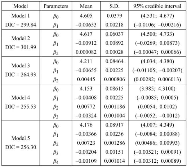
Using the WinBugs software, we first simulated a “burn-in-sample” size of 10,000, discarded to eliminate the effect of the initial values used in the Gibbs sampling algorithm. After this “burn-in-sample period”, we simulated another 20,000 Gibbs “burn-in-samples forβ0andβ1. From this sample, we selected a final sample size of 1,000, taking a sample chosen from every 20 simulated samples to have an approximately uncorrelated sample to be used to find the posterior summaries of interest. The obtained posterior summaries of interest (posterior mean, posterior standard deviation, and 0.95% credible intervals) are given in Table 2. Convergence of the algorithm was monitored using standard trace plots from the simulated samples (see, for example, Paulinoet al., 2003, or Gamerman, 1997).
In Table 2, we also have the posterior summaries of interest considering the models 2, 3, 4 and 5 assuming the same normal prior distributions N(0,10)for the regression parametersβj,
j =1,2,3,4.
In the simulation of Gibbs samples for the parameters of these models we used the same steps in the WinBugs software used for model 1.
For selection of the best model to be fitted by the data, three discrimination criteria were consid-ered:
(a) Graphical verification of the fit: in this case, plots of the observed values yi were consid-ered (counting of units sent to quality control on thei-th day) against days and plots of the fitted means (posterior mean ofλiin (1)) considering the five proposed models.
Table 2– Posterior summaries.
Model Parameters Mean S.D. 95% credible interval
Model 1 β0 4.605 0.0379 (4.531; 4.677)
DIC = 299.84 β1 –0.00653 0.00218 (–0.0106; –0.00216)
Model 2 β0 4.617 0.06037 (4.500; 4.733)
DIC = 301.99 β1 –0.00912 0.00892 (–0.0269; 0.00873)
β2 0.000082 0.00028 (–0.00047; 0.00066)
Model 3 β0 4.211 0.08464 (4.034; 4.380)
DIC = 264.93 β1 –0.00655 0.00225 (–0.01105; –0.00207)
β2 0.00445 0.000806 (0.00282; 0.006013)
β0 4.153 0.08615 (3.985; 4.3100)
Model 4 β1 –0.00408 0.00225 (–0.0085; 0.0005)
DIC = 255.53 β2 0.00772 0.001186 (0.0054; 0.0102)
β3 –0.00324 0.001004 (–0.0052; –0.0012)
β0 4.176 0.08917 (4.007; 4.349)
Model 5 β1 –0.00366 0.00236 (–0.0084; 0.00088)
DIC = 256.30 β2 0.00723 0.001286 (0.00486; 0.00993)
β3 –0.00204 0.00151 (–0.00521; 0.00091) β4 –0.00109 0.001014 (–0.00312; 0.00089)
Source: Author’s own.
(c) Determination of the sums of the absolute values of the differences between the observed valuesyiwith the fitted values (posterior means ofYi),i =1,2, . . . ,30, that is
Sj = 30
X
i=1
|yi− ˇλi| (9)
where yi is the daily counting of units sent to quality control and λiˇ is the Monte Carlo
estimate of the posterior mean forλibased on the 1,000 simulated Gibbs samples.
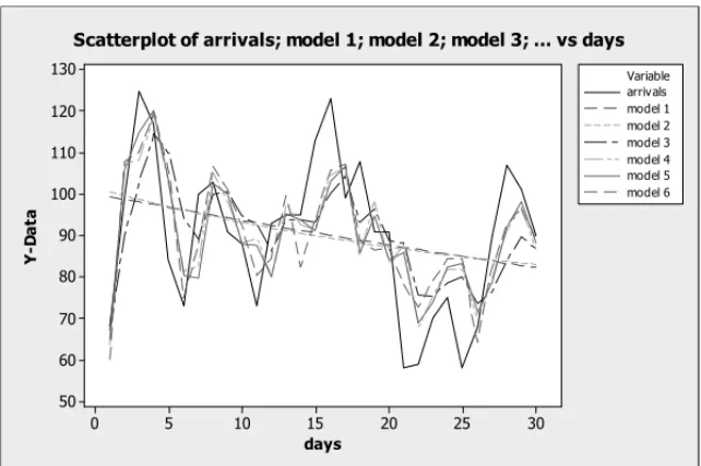
In Figure 2, we have the graphs of the observed values yi against days and the graphs of the
estimated values (λiˇ ) against days, fori =1,2, . . . ,30. We observe that models 4 and 5 have a good fit for the counting data presented in Table 1. We also observe smaller values for DIC (see Table 2) assuming models 4 and 5, an indication of better models.
Considering the sums of the absolute values of the differences between the observed values yi
30 25 20 15 10 5 0 130
120
110
100
90
80
70
60
50
Variable
model 4 model 5 model 6 arriv als model 1 model 2 model 3
Figure 2 – Graphs of observed and fitted values against days
Figure 2– Graphs of observed and fitted values against days.
Assuming model 4 (a model with fewer parameters), the presence of an indicator or “dummy” variable for weekday was considered; that is, Zi = 1 for Mondays and Zi = 0 for the other
weekdays and the regression Poisson model (“model 6”) given by
λ1=exp(β0+β1X1+β4Z1) λ2=exp(β0+β1X2+β2y1+β4Z2) λi =exp(β0+β1Xi+β2yi−1+β3yi−2+β4Zi)
(10)
wherei =3,4, . . . ,30.
In Table 3, the posterior summaries of interest are given for model 6 defined by (1) and (10) assuming normal prior distributions with variance equals to 10, and the same simulation steps considered for the other models using the WinBugs software.
Table 3– Posterior summaries (“model 6”).
Parameter Mean S.D. 95% credible interval
β0 4.245 0.09352 (4.060; 4.427)
β1 –0.00475 0.00240 (–0.00912; 0.000197) β2 0.006532 0.00124 (0.00414; 0.00899) β3 –0.00259 0.000984 (–0.0044; –0.00068) β4 –0.1462 0.05147 (–0.2489; –0.0452)
Source: Author’s own.
4 DISCUSSION OF THE RESULTS OBTAINED
From the results obtained from Table 3, for “model 6”, we observe that the co-variates yi−1 (counting with a lag of one day), yi−2 (counting with a lag of two days) and Zi (weekday)
present significant effects in the daily counting of units sent to quality control, since the zero value is not included in the 95% credible intervals for the regression parametersβ2,β3andβ4. Since the Bayesian estimate of the parameterβ4is negative(βˆ4 = −0.1462), we observe that Mondays present smaller counting of units sent to quality control as compared with the other weekdays. This result could be of great interest for the company.
It was also possible to use “model 6” to get predictions, from the fitted model (11):
(λiˇ )=exp(4.245−0.00475Xi+0.00653yi−1−0.00259yi−2−0.1462Zi) (11)
So, considering the prediction for future days(i =31), we haveX31=31,y30=90,y29=101, Zi =1 (if the next day is a Monday); that is,(λˇ31)=72.0716 (72 units); ifZi =0 (the next day
is not a Monday), we haveλˇ31=83.4177 (83 units).
These results are important for the company in planning human resources in the quality control department due to a low utilization rate, especially on Mondays. Capacity planning could be done using a customized calendar for Mondays when running Discrete Event Simulation. Finally, in Table 4, we have the observed values (arrivals) and the fitted values for the means assuming each proposed model. Observe that our Bayesian estimates in Table 4 are given by Monte Carlo estimates of the posterior means based on the simulated Gibbs samples for each parameter. Under the Bayesian paradigm, we usually base our inferences on credibility intervals, rather than using hypothesis tests, as is common from a classical Bayesian perspective.
5 FINAL CONSIDERATIONS
Table 4– observed values and estimated means.
Observation Arrivals Model-1 Model-2 Model-3 Model-4 Model-5 Model-6
1 68 99.42 100.50 67.21 63.62 65.12 60.20
2 99 98.77 99.54 90.14 107 105.90 108.00
3 125 98.12 98.65 102.80 108.30 114.90 110.10
4 117 97.48 97.79 114.70 119.20 120.30 119.90
5 84 96.84 96.97 109.90 102.60 103.70 105.90
6 73 96.20 96.16 94.25 81.33 80.41 74.97
7 100 95.57 95.39 89.17 82.77 79.83 87.48
8 103 94.95 94.64 99.89 105.20 102.50 106.80
9 91 94.33 93.91 100.60 98.22 99.92 101.10
10 88 93.71 93.20 94.71 88.31 88.08 92.32
11 73 93.10 92.52 92.84 89.34 87.71 80.33
12 93 92.49 91.85 86.28 80.04 79.94 84.53
13 95 91.89 91.21 93.69 97.64 95.21 99.64
14 95 91.29 90.58 93.91 92.54 93.91 82.48
15 113 90.69 89.98 93.30 91.57 91.16 94.45
16 123 90.10 89.39 100.40 104.80 103.20 105.70
17 99 89.52 88.82 104.30 106.40 106.60 107.20
18 108 88.93 88.27 93.13 85.22 85.80 88.93
19 91 88.36 87.73 96.31 98.32 94.78 86.36
20 91 87.78 87.21 88.70 83.41 84.15 86.90
21 58 87.21 86.72 88.13 87.77 85.94 78.13
22 59 86.65 86.23 75.61 67.81 68.78 72.57
23 70 86.09 85.77 75.46 75.73 73.80 79.15
24 75 85.53 85.33 78.71 81.83 82.36 84.41
25 58 84.98 84.90 79.96 81.73 83.11 84.35
26 68 84.43 84.49 73.67 70.26 71.65 64.12
27 90 83.88 84.11 76.51 79.87 78.98 82.36
28 107 83.34 83.74 83.83 91.26 92.11 92.22
29 101 82.80 83.39 89.85 96.49 98.16 96.89
30 90 82.27 83.07 86.91 86.81 88.30 88.72
Source: Author’s own.
observed in our application. A better model means a better forecast, which is of great interest for industrial managers.
REFERENCES
[1] ALBERTJ. 1992. A Bayesian analysis of a Poisson random-efects model.American Statistician,46: 246–253.
[2] ANDRADOTTIR´ S & BIERVM. 2000. Applying Bayesian ideas in simulation.Simulation Practice and Theory,8: 253–280.
[3] ARMSTRONGJS & FILDESR. 2006. Making process in forecasting.International Journal of Fore-casting,22: 433–441.
[4] BAROSSI-FILHO M, ACHCAR JA & SOUZARM. 2010. Modelos de volatilidade estoc´astica em s´eries financeiras: uma aplicac¸˜ao para o IBOVESPA.Economia Aplicada,14(1): 25–40.
[5] BLUNDELLR, GRIFFITHR & VANREENENJ. 1995. Dynamic count models of technological Inno-vation.Economic Journal,105: 333–344.
[6] BOXG & TIAOG. 1973. Bayesian inference in statistical analysis. New York: Addison-Wesley.
[7] CAMERONAC & TRIVEDIPK. 1998. Regression Analysis of Count Data. New York: Cambridge University Press.
[8] CAVALCANTECAV & ALMEIDAAT. 2011. Modelo multicrit´erio de apoio a decis˜ao para o plane-jamento de manutenc¸˜ao preventiva utilizando PROMETHEE II em situac¸ ˜oes de incerteza.Pesquisa Operacional,25(2): 279–296.
[9] CHEX & XU S. 2011. Bayesian data analysis for agricultural experiments.Canadian Journal of Plant Science,91(4): 599–601.
[10] CHIBS & GREENBERGE. 1995. Understanding the Metropolis-Hastings algorithm.The American Statistician,49: 327–335.
[11] CHIBS, GREENBERGE & RAINERW. 1998. Posterior simulation and Bayes factors in panel count data models.Journal of Econometrics,86: 33–54.
[12] DROGUETTEL & MOSLEHA. 2011. An´alise bayesiana da confiabilidade de produtos em desen-volvimento.Gest˜ao da Produc¸˜ao,13(1): 57–69.
[13] FERREIRARJP, ALMEIDAFILHOAT & SOUZAFMC. 2009. A decision model for portfolio selec-tion.Pesquisa Operacional,29(2): 403–417.
[14] FILDES R. 2006. The forecasting journals and their contribution to forecasting research: Citation analysis and expert opinion.International Journal of forecasting,22: 415–432.
[15] FREELANDRK & MCCABEBPM. 2004a. Forecasting discrete valued low count time series. Inter-national Journal of Forecasting,20: 427–434.
[16] FREELANDRK & MCCABEBPM. 2004b. Analysis of low count time series data by Poisson autore-gression.Journal of Time Series Analysis,25: 701–722.
[17] FREITAS MA, COLOSIMO EA, SANTOS TR & PIRES MC. 2010. Reliability assessment using degradation models: Bayesian and classical approaches.Pesquisa Operacional,30(1): 195–219.
[18] GAMERMAN D. 1997. Markov Chain Monte Carlo: stochastic simulation for Bayesian inference. London: Chapman and Hall.
[20] GROSSD & HARRISCM. 1974. Fundamentals of queueing theory. New York, USA: John Wiley & Sons.
[21] GURMUS, RILSTONEP & STERNS. 1999. Semiparametric estimation of count regressionmodels. Journal of Econometrics,88: 123–150.
[22] HARVEYAC & FERNANDES C. 1989. Time series models for count or qualitative observations. Journal of Business and Economic Statistics,7: 407–417.
[23] HAUSMANJA, HALLBH & GRILICHESZ. 1984. Econometric models for count data with applica-tions to the patents R and D relaapplica-tionship.Econometrica,52: 909–938.
[24] HSUL-C & WANGC-H. 2007. Forecasting the output of integrated circuit industry using a grey-model improved by the Bayesian analysis.Technological Forecasting & Social Change,74: 843–853.
[25] KALATZISAEG, AZZONICR & ACHCARJA. 2006. Uma abordagem bayesiana para decis ˜oes de investimentos.Pesquisa Operacional,26(3): 585–604.
[26] KARIHH, SALINAS J & LOMBARDI F. 1994. Generating non-standard random distributions for discrete event simulation systems.Simulation Practice and Theory,1: 173–193.
[27] KELTONWD, SADOWSKIRP & STURROCKDT. 2007. Simulation with Arena. Forth Edition. New York, USA: McGraw-Hill.
[28] KLEINROCKL. 1975. Queueing systems. Vol. 1: Theory. New York, USA: John Wiley & Sons.
[29] LARSON R & ODONIA. 1981. Urban Operations Research. New Jersey, USA: Prentice Hall Inc. Englewood Cliffs.
[30] LEEMISLM. 2006. Arrival Processes, Random Lifetimes and Random Objects. In: Handbooks in Operations Research and Management Science, Volume 13: Simulation [edited by HENDERSONSG ANDNELSONBL], North Holland, 155–180.
[31] MARTZHF & HAMADAMS. 2003. Uncertainty in counts and operationg time in estimating Poisson occurence rates.Reliability Engineering & System Safety,80: 75–79.
[32] MARTZ HF & PICARDRR. 1995. Uncertainty in Poisson event counts and exposure time in rate estimation.Reliability Engineering & System Safety,48: 181–90.
[33] MCCABEBPM & MARTINGM. 2005. Bayesian predictions of low count time series.International Journal of Forecasting,21: 315–330.
[34] MOTTAJ. 1997. Decis˜oes de prec¸o em clima de incerteza: uma contribuic¸˜ao da an´alise Bayesiana. Revista de Administrac¸˜ao de Empresas,37(2): 31–46.
[35] MOURAMC, ROCHASPV & DROGUETTEL. 2007. Avaliac¸˜ao Bayesiana da efic´acia da manuten-c¸˜ao via processo de renovamanuten-c¸˜ao generalizado.Pesquisa Operacional,27(3): 569–589.
[36] PAULINO CD, TURKMAN M & MURTEIRA B. 2003. Estat´ıstica Bayesiana. Lisboa: Fundac¸˜ao Calouste Gulbenkian.
[37] PONGORMR & BUENONETOPR. 1997. Uma metodologia bayesiana para estudos de confiabili-dade na fase de projeto: aplicac¸˜ao em um produto eletr ˆonico.Gest˜ao da Produc¸˜ao,4(3): 305–320.
[39] SETTIMIR & SMITH JQ. 2000. A comparison of approximate Bayesian forecasting methods for non-Gaussian time series.Journal of Forecasting,19: 135–148.
[40] SPIEGELHALTERDJ, THOMASA, BEST NG & LUNND. 2003. WinBugs: user manual, version 1.4. Cambridge, U.K.: MRC Biostatistics Unit.
[41] SPIEGELHALTERDJ, BESTNG, CARLINBP &VAN DERLINDEA. 2002. Bayesian measures of model complexity and fit.Journal of the Royal Statistical Society, series B,64(4): 583–639.
[42] YANGF & LIUJ. 2012. Simulation-based transfer function modeling for transient analysis of general queueing systems.European Journal of Operational Research,
http://dx.doi.org/10.1016/j.ejor.2012.05.040. Accessed on June 26, 2012.
[43] ZEGERSL. 1988. A regression model for time series of counts.Biometrika,75: 621–629.
[44] ZHANGH, TAMCM & LEEH. 2005. Modeling uncertain activity duration by fuzzy number and discrete-event simulation.European Journal of Operational Research,164: 715–729.
[45] ZHENGX. 2008. Semiparametric Bayesian estimation of mixed count regression models.Economic