Aerosol model selection and uncertainty modelling by adaptive MCMC technique

(1)

ACPD

8, 10791–10816, 2008

Aerosol model selection

M. Laine and J. Tamminen

Title Page

Abstract Introduction

Conclusions References

Tables Figures

◭ ◮

Back Close

Full Screen / Esc

Printer-friendly Version

Interactive Discussion Atmos. Chem. Phys. Discuss., 8, 10791–10816, 2008

www.atmos-chem-phys-discuss.net/8/10791/2008/ © Author(s) 2008. This work is distributed under the Creative Commons Attribution 3.0 License.

Atmospheric Chemistry and Physics Discussions

Aerosol model selection and uncertainty

modelling by adaptive MCMC technique

M. Laine and J. Tamminen

Finnish Meteorological Institute, Helsinki, Finland

Received: 20 February 2008 – Accepted: 14 May 2008 – Published: 5 June 2008

Correspondence to: M. Laine (marko.laine@fmi.fi)

(2)

ACPD

8, 10791–10816, 2008

Title Page

Tables Figures

◭ ◮

Back Close

Full Screen / Esc

Interactive Discussion

Abstract

We apply Bayesian model selection techniques on the statistical inversion problem of the GOMOS instrument. The motif is to study which type of aerosol model best fits the data and to show how the uncertainty of the aerosol model can be included in the error estimates. The competing models consist of various formulations, each having different

5

unknown parameter vectors. We have developed an Adaptive Automatic Reversible Jump Markov chain Monte Carlo method (AARJ) for sampling values from the posterior distributions of the unknowns of the models. The algorithm is easy to implement and can readily be employed for model selection as well as for model averaging, to properly take into account the uncertainty of the modelling.

10

1 Introduction

Advances in computer resources and algorithms have made possible the use of in-creasingly complicated models. In geophysical sciences the estimation of unknowns in large models is commonly handled using linearizations and approximations that can effect the uncertainty estimates of the retrievals. Bayesian inference provides a unified

15

and natural framework to consider uncertainty in the estimated values as well as the model uncertainty. In many cases, classical approximative estimation methods can be seen as special cases of some more general Bayesian analyses, see for example Kaipio and Somersalo (2004).

In Bayesian inference, the uncertainty of the estimated value is a primary target of the

20

investigation. Whenever computationally possible, the result of the analysis is the full multi-dimensional posterior probability density of the unknowns. The approach allow the study of many kinds of uncertainties, including uncertainty in the model itself. Prior information from different sources can be pooled and incorporated statistically correctly and the correlation structure of the unknowns can be fully explored. Practical tools for

25

applying Bayesian inference to modelling problems are provided by the Markov chain

(3)

ACPD

8, 10791–10816, 2008

Title Page

Tables Figures

◭ ◮

Back Close

Full Screen / Esc

Interactive Discussion Monte Carlo (MCMC) methods. MCMC is a common title for algorithms that simulate

values from a probability distribution known only up to a normalizing constant. A typical case of such a task is to find the posterior distribution of the unknown parameters of a geophysical model. For application examples and more details on applying Bayesian MCMC methods in geophysical research see, for example, Tamminen and Kyrl (2001);

5

Tamminen (2004); Haario et al. (2004).

In this article the Bayesian model selection and averaging is applied to the GOMOS (ESA 2007) aerosol model selection problem. GOMOS (Global Ozone Monitoring by Occultation of Stars) is an instrument on board the Envisat satellite that uses stellar oc-cultation to measure the atmosphere (http://envisat.esa.int/instruments/gomos/). The

10

aerosol cross-section model in the GOMOS retrieval algorithm is just an approximation of the underlying aerosol extinction process. Indeed, several alternative formulations are possible, depending on the types of the aerosols at a given location. Consequently, it is advisable to allow for di_fferent types of models and let the data decide which one to use. By adaptive MCMC methods this can be done as a part of general estimation

15

procedure in a statistically correct manner.

This article introduces an adaptive MCMC method, called AARJ, for model selec-tion problems. AARJ is an easy to use and efficient version of the Reversibe Jump MCMC algorithm. We demonstrate the technique in the aerosol model selection of the GOMOS remote sensing instrument, but we emphasize that the method is

gen-20

eral and applicable to general model selection problems. The structure of this article is the following. In Sect. 2 the basics of Bayesian model selection are reviewed. In Sect. 3 the MCMC method for simulating from a posterior distribution of model param-eters is explained and an adaptive automatic reversible jump MCMC algorithm (AARJ) is introduced. The algorithm can be used for model determination problems where a

25

(4)

ACPD

8, 10791–10816, 2008

Title Page

Tables Figures

◭ ◮

Back Close

Full Screen / Esc

2 Bayesian model selection

Choosing the right model is a complicated matter. The problem can not, clearly, be solved by purely statistical considerations. The researchers insight into the subject matter will always be the most valuable resource. Statistical methods can, however, tell if the chosen models and modelling assumptions are highly unprobable for the

situ-5

ation and calculate relative merits of different modelling approaches. Here we present statistical methods that are able to tell which of the possible solutions o_ffer the best fit given the set of models to consider, the data observed, and the prior information that is available.

In many cases the ground truth is unknown. We could have several speculative

alter-10

natives about the physical behavior of the system, e.g. depending on some unknown state of nature at the location under consideration. Then it is reasonable to model also the uncertainty in the model, for example by introducing several alternative models and let the data decide which of them to use. A problem, similar to a point estimation (or maximum a posteriori estimation) in parameter estimation, would then be the selection

15

of the best model. If no single model stands out, then this uncertainty can be taken into account in the results by averaging the predictions over the models according to their posterior weights.

We briefly introduce the main concepts of model determination in the Bayesian framework and discuss various probability distributions of the unknowns concerned.

20

Letx stand for a vector of unknown variables of primary interest andη(k) for extra un-known model parameters in thek:th model. We assume thatx is common to all the models. We want to use the observed data, y, to estimate the unknowns x and η(k)

and also make inference about the unknown modelk. In our case, the model indexk

is a label for a finite set of pre-selected models. In the GOMOS example presented in

25

Sect. 4 symbolx will stand for the constituent the line densities andη(k) contains the aerosol cross-section parameters for four cross-section modelsk=1, . . . ,4.

To apply Bayesian inference we need to assign prior probabilities jointly for all the

(5)

ACPD

8, 10791–10816, 2008

Title Page

Tables Figures

◭ ◮

Back Close

Full Screen / Esc

Interactive Discussion unknowns,p(x, η(k), k). It can be written as a product of conditional probabilities

p(x, η(k), k)=p(x|η(k), k)p(η(k)|k)p(k). (1)

This formulation reveals the hierarchical structure of the unknowns. Priors can be given sequentially by first assigning prior probabilities for di_fferent models, p(k), then prior distributions for the model parametersp(η(k)|k) in each model and lastly the priors for

5

the unknown variablesp(x_|η(k)). In addition, we must formulate the likelihood function,

p(y|x, η(k), k), giving the distribution of the observations, using the forward model and the statistical description of the observational error.

The joint posterior distribution of the unknownsx, η(k) and k conditional to the ob-served datay is written by the aid of the Bayes formula and is expressed as a product

10

of the likelihood and the priors:

p(x, η(k), k_|y)= p(y|x, η

(k)

, k)p(x|η(k), k)p(η(k)|k)p(k)

p(y) . (2)

For the actual calculation of the posterior density we must solve the well known problem of computing the unconditional probability of the observationsp(y) in the denominator of the Bayes formula. As the observed data y are fixed, the termp(y) can be seen

15

as a normalizing constant that makes the product of likelihood and prior to become a probability density function. This means that we can write

p(y)₌

Z

p(y|x, η(k), k)p(x|η(k), k)p(η(k)|k)p(k)d(x, η(k), k) (3)

and the calculation involves averaging over all the unknown variables of the model, making it into an integration problem with dimension equal to the number of unknowns

20

(6)

ACPD

8, 10791–10816, 2008

Title Page

Tables Figures

◭ ◮

Back Close

Full Screen / Esc

Interactive Discussion Let us next consider the problem of selecting the best modelkfrom a set of

compet-ing models. Di_fferent models can be judged according to the evidence they give to the observations, i.e. we consider the probabilities:

p(y|k)=

Z

p(y|θ(k), k)p(θ(k)|k)p(k)d θ(k), (4)

whereθ(k)=(x, η(k)) is used as a shorthand for the vector of all unknowns of the model

5

k. The posterior model probabilities can be written using the Bayes formula as

p(k|y)=p(y|k)p(k)

p(y) . (5)

If the values above are available, then model comparisons can be done using posterior odds:

p(k1|y)

p(k2|y)

= p(y|k1)

p(y|k2)

p(k1)

p(k2)

, (6)

10

where the first term in the right,p(y_|k1)/p(y|k2), is called the Bayes factor, the relative evidence of modelk1wrt. modelk2given by the datay andp(k1)/p(k2) is the ratio of prior model probabilities.

The calculation of model probabilityp(k_|y), and that of the evidence p(y_|k), poses challenges, especially if the class of models considered is large and if there is no

15

natural hierarchy between the models that could be exploited. Several methods for the calculations have been proposed, either by using approximations that avoid the problems of high dimensional integration, or by using results of the MCMC runs on the individual models. The adaptive RJMCMC method, AARJ, presented below allows for a simple method of calculating the model posterior probabilities from an MCMC

20

simulation done simultaneously over all the selected models.

(7)

ACPD

8, 10791–10816, 2008

Title Page

Tables Figures

◭ ◮

Back Close

Full Screen / Esc

3 Markov chain Monte Carlo – MCMC

In the most general setting we are interested in the whole posterior distribution of all the unknowns. Sometimes we are satisfied with some statistics of the distribution, such as the mean and standard deviation. The calculation of most statistics will lead, in general, to a high dimensional integration problem that has no closed form solutions.

5

The Monte Carlo methods use random numbers to replace the integrals with sample averages that are easy to calculate. But even the standard Monte Carlo techniques using independent random variables are in trouble when the dimension is higher than 3 or 4. The solution offered by the Markov chain Monte Carlo (MCMC) methods is to use high dimensional random walks.

10

The most important MCMC algorithm is the Metropolis-Hasting (MH) algorithm. It has several useful generalizations and important special cases for different purposes. The MH algorithm for sampling from a posterior distributionp(θ|y) can be described as follows. Again, we letθstand for all the unknowns of our model, including unknown state variables, model parameters and the model index, θ=(x, η(k), k). Starting from

15

an initial guessθ0 we generate a chain of possible parameter realizationsθ0, θ1, . . .. In each step i with a current value θi we propose a new value θ∗ using a proposal

distributionq(θ_i,·). As the notation suggests, this proposal can depend on the current valueθ_i. The proposal could be, for example, a multi dimensional Gaussian distribution centered at the current value θi. The new value is accepted using an acceptance 20

probability α(θ_i, θ∗) that depends on the ratio of the posteriors and on the chosen proposal distribution:

α(θ_i, θ∗)=min

1,p(θ

∗_|_y₎_q₍_θ∗_{, θ}

i) p(θ_i_|y)q(θ_i, θ∗₎

=min

1,p(y|θ

∗₎_p₍_θ∗₎_q₍_θ∗_{, θ}

i) p(y_|θ_i)p(θ_i)q(θ_i, θ∗₎

. (7)

Ifθ∗ is accepted, we setθ_i₊1=θ∗, otherwise the chain stays at the current value, that isθi+1=θi. If the proposal is symmetric, q(θi, θ∗)=q(θ∗, θi), as it is the case with the 25

(8)

ACPD

8, 10791–10816, 2008

Title Page

Tables Figures

◭ ◮

Back Close

Full Screen / Esc

Interactive Discussion unconditionally if it is better than the previous value, i.e., ifp(θ∗|y)/p(θi|y)>1. If it is

not better in the above sense, thenθ∗is accepted with a probability that is equal to the posterior ratiop(θ∗_|y)/p(θ_i_|y). The MH algorithm can be thought as a random walker travelling uphill towards the peak of the posterior distribution, but frequently taking steps downhill, too.

5

The basic idea behind the MH algorithm is that instead of computing the values of the posteriorp(θ|y) directly, we only need to compute ratios of the posteriors at two distinct parameter values,p(θ2|y)/p(θ1|y). This cancels out the normalizing constant

p(y) and the parts of the likelihood function p(y_|θ) that do not depend on θ. Using standard Markov chain theory (for example Gamerman, 1997), it can be shown that

10

this algorithm produces a chain of values whose distribution approaches the target posterior distributionp(θ_|y). We might need to allow some burn-in time to let the chain reach the limiting distribution.

After the MCMC run we have a chain of values of the parameter vector at our dis-posal. The inference about the unknowns is done with statistics calculated by the

15

chain. The mean of the chain is a Bayesian point estimate for the unknown, a his-togram or a kernel density gives an estimate for the marginal posterior density. If we think of the generated chain as a matrix where the number of rows corresponds to the size of the MCMC sample and the number of columns corresponds to the number of unknowns in the model, then each row is a possible realization of the model and these

20

appear in correct proportions corresponding to the posterior distribution. Plotting one-dimensional or two-one-dimensional scatter plots of the sampled parameter values from the chain produces representations of the respective marginal posterior densities.

3.1 Reversible jump MCMC

To include model selection into the MCMC framework a modification to the basic

25

Metropolis-Hastings algorithm outlined above is needed. If we want the MCMC chain to explore different models and parametrizations, we must somehow allow the dimen-sion of the unknown to change. This is the motivation behind the Reversible Jump

(9)

ACPD

8, 10791–10816, 2008

Title Page

Tables Figures

◭ ◮

Back Close

Full Screen / Esc

Interactive Discussion MCMC (RJMCMC) algorithm by Green (1995). In the RJMCMC algorithm the proposal

distribution and the acceptance probability are formulated in such a way that the chain can perform reversible jumps between spaces of different dimensions. This means, es-pecially, that the random walk of the MH algorithm can simultaneously explore different models for the same data.

5

The RJMCMC algorithm can be presented in theoretical framework that extends the standard MH algorithm to a more general state space of the unknowns. We will not present the general theory, but refer to Green (1995). Instead, we show how the method can be succesfully implemented in a situation where we consider several dif-ferent models for the same data. This approach is also based on the work of Green

10

(2003) and is called automatic RJMCMC.

In automatic RJMCMC a special MCMC sampler is constructed that can jump be-tween different models. For the MCMC chain to move from one model to another, we need a way to transform the model parameters. A simple but general way to do this this is the following. Suppose that for each modelk, the target posterior distributions can

15

be approximated by a mean vector µ_k and a covariance matrix C_k=R_kTR_k, where R_k

denotes the Cholesky decomposition factor. These approximations are used to trans-form the unknowns in each model into approximately independent Gaussian variables and they thus provide a common scale to perform the between model transformations of the parameters. Additionally, as seen below, the covariance matrixCk can be used 20

to form the proposal distribution of the Metropolis-Hastings step of the algorithm. Let again θ(k) stand for the vector of all the unknowns in the model k and let the dimension ofθ(k) ben_k. Assume that the chain is currently in the modeli. Using the vectorµ_i and the matrix R_i, we can compute a scaled and normalized version of the current chain value as

25

zi =(θ(i)−µi)R_i−1. (8)

(10)

ACPD

8, 10791–10816, 2008

M. Laine and J. Tamminen Title Page Abstract Introduction Conclusions References Tables Figures ◭ ◮ ◭ ◮ Back Close

Full Screen / Esc

Interactive Discussion transformation from the model spacei to the model spacej as

θ(j)=µ_j +z_iR_j. (9)

If the dimensions of the two models do not match, we either drop some columns ofzi or

add new dimensions to it using independent Gaussian random numbers,u_∼ N(0, I). The transformations can be written as

5

θ(j)=

          

µj +[zi] nj

1 Rj ifni > nj

µ_j +z_iR_j ifn_i =n_j

µ_j +

"

z_i u

#

R_j ifn_i < n_j.

(10)

Here [z]i₁means the firsti components of the vectorz.

The Metropolis-Hastings acceptance probability for a move from the modeli to the modelj and from a parameter value θ(i) to that of θ(j) is calculated according to the RJMCMC theory. Letp(i , j) be the probability to propose a jump to the modelj when

10

the chain is currently at the modeli, i.e., if the current model isi then the next model is chosen with a draw from a proposal distributionp(i ,_·). If the modelj is selected, then the current parameter vector is transformed to the new model according to Eq. (10). The acceptance probability for the RJMCMC sampler can be written as

α(θ(i), θ(j))₌max 1,p(y|θ

(j)

, j)p(θ(j), j)p(j, i)

p(y_|θ(i)_{, i}₎_p₍_θ(i)_{, i}₎_p₍_{i , j}₎

R_j

|Ri| g

!

, (11)

15

where_|R_|is the determinant of the matrixR and the last term gdepends on the extra variableuand is given as

g=φ(u) ifni > nj, (12)

1 ifn_i =n_j, (13)

φ(u)−1ifni < nj, (14)

20

(11)

ACPD

8, 10791–10816, 2008

Title Page

Tables Figures

◭ ◮

Back Close

Full Screen / Esc

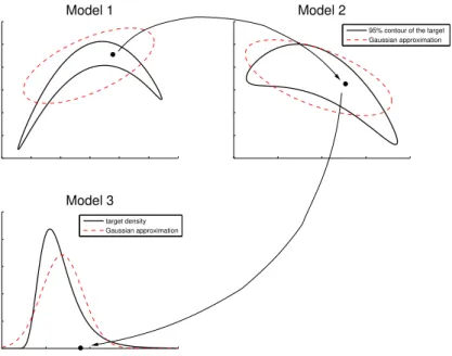
Interactive Discussion whereφis the probability density function of independent multi dimensional Gaussian

values, N(0, I). Figure 1 illustrates the model moves. Note that when moving from one model to another with equal dimension, the transformation is totally deterministic, no random variables are used to make the move. To introduce more randomness, Green (2003) suggests a random permutation of the components of the normalized

5

z variables at each step. This permutation, if used, does not change the acceptance probability.

For a move inside the same model we use a Gaussian proposal distribution and the standard MH acceptance probability Eq. (7). The approximation of the posterior provided by the matrix C_i=R_iTR_i is used to make the proposal to have a correlation

10

structure similar to that of the target distribution. Ifξis a random vector of independent Gaussian random variablesξ_∼N(0, I_n_i), then the proposed value can be written as

θ(i)∗ =θ(i)+ξRi

√

s, (15)

wheres=2.42/n_i is a scaling factor. The acceptance probability Eq. (11) simplifies to that of the standard MH algorithm for symmetric proposal.

15

This sampler is easy to implement. The success of it depends on how well the Gaussian approximations are able to provide decent proposals for moves from model to model. It is, however, typical in many geophysical applications to have parameter posteriors close to Gaussian. This also is the reason why the classical estimation methods often work quite well. But the use of RJMCMC allows us to incorporate model

20

selection methods together with prior information, such as positivity or smoothness constraints, in a statistically sound manner. Also, we are able to properly deal with nonlinear correlation structures that usually are not found by the classical methods.

3.2 Adaptive automatic RJMCMC – AARJ

From a practical point of view the problem with the standard MCMC algorithms is that,

25

(12)

ACPD

8, 10791–10816, 2008

Title Page

Tables Figures

◭ ◮

Back Close

Full Screen / Esc

Interactive Discussion specific tuning. The most important aspect is the choice of the proposal distributions

q. In the Metropolis-Hastings algorithm the proposal can, at least in theory, be quite arbitrary. Choosing a distribution that closely resembles the true posterior distribution can dramatically speed up the convergence of the generated values to the right distri-bution. The closer the proposal distribution is to the actual posterior distributionp(θ|y),

5

the better the chain “mixes” and the better a short sequence represents a draw from the posterior. This is especially true in multidimensional cases and when the compo-nents of the parameter vector are correlated. A general and computationally e_fficient choice for the proposal distribution is the multidimensional Gaussian density. As the shape of the Gaussian density is determined by its covariance matrix, the tuning of the

10

algorithm in this case means the selection of the covariance.

In the basic MH algorithm the proposal distribution must not depend on the values generated so far, except for the current value. This is the requirement behind the Markov property of the stochastic process that the MCMC sampler defines. If we allow for adaptation depending on the history, the convergence theorems based on Markov

15

chain theory must be checked. Numerous adaptive strategies for the choice of the proposal distribution have been suggested. In our experiences, the Adaptive Metropolis (AM) and the Delayed Rejection Adaptive Metropolis (DRAM) have proved to perform well in several geophysical and environmental modelling applications (Haario et al., 2001, 2006, 2004). These two methods are the building blocks for the new adaptive

20

RJMCMC method presented below, for which we use the acronym AARJ.

In the AM adaptation the Gaussian proposal distribution is tuned using an increasing part of the chain values generated so far. In Haario et al. (2001) this method is shown to be ergodic, so it can be used to accurately sample from the target distribution. A recursive formula for the covariance matrix can be used to ease the computations. The

25

DRAM adaptation (Haario et al., 2006) adds a new component to the AM method that is called Delayed Rejection (DR, Mira, 2001). In the DR method, instead of one proposal distribution we can have several proposals. These can be used in turn, until a new value is accepted. The DR acceptance probability formulation ensures that the generated

(13)

ACPD

8, 10791–10816, 2008

Title Page

Tables Figures

◭ ◮

Back Close

Full Screen / Esc

Interactive Discussion chain is Markovian and that the so called reversibility condition holds. This means that

all the standard MH distributional convergence statements hold. In the DRAM method the DR algorithm is used together with several different adaptive Gaussian proposals. This helps the algorithm in two ways. Firstly, it enhances the adaptation by providing accepted values that make the adaptation start earlier. Secondly, it allows the sampler

5

to work better for non Gaussian targets and with non linear correlations between the components. The ergodicity of the DRAM method is proven by Haario et al. (2006).

A new feature presented in this article is the combination of the DRAM and AM adaptations with the automatic RJMCMC. The practical application presented is the aerosol model selection in the GOMOS inversion. We want to note that Hastie (2005)

10

has also suggested a combination of adaptation and automatic RJMCMC of Green. The adaptation method (so called Adaptive Acceptance Probability, AAP) used in his work is, however, different from the adaptation employed here. We regard our AARJ method to be more general and easily applicable to high dimensional nonlinear models typical in geophysical problems.

15

3.3 The AARJ algorithm

Here we present a schema for the algorithm for AARJ, an Adaptive Automatic Re-versible Jump MCMC for model selection and model averagingl problems with a fixed number of modelsM1, . . . , Mk.

3.3.1 The algorithm

20

1. Run separate adaptive MCMC chains using the DRAM method for all the pro-posed models. Collect the mean vectorsµ(i) and the Cholesky factorsR(i)of the covariance matrices of the chains,i=1, . . . , k.

2. Run automatic RJMCMC using the target approximations calculated in step (1).

3. If the current model is kept, use the standard random walk MH with Gaussian

(14)

ACPD

8, 10791–10816, 2008

Title Page

Tables Figures

◭ ◮

Back Close

Full Screen / Esc

Interactive Discussion posal distribution such that the proposal covariance depends onR_i in the current

model.

4. After given (random or fixed) intervals, adapt each model approximation by the AM method using those parts of the chain generated so far that belong to the particular model.

5

The AARJ method is easy to implement. For example, a computer program running the basic Metropolis-Hasting MCMC simulation can readily be extended to do both DRAM and AARJ. The GOMOS application example below has been coded in Matlab programming environment, using a MCMC toolbox for Matlab (Laine, 2008).

4 Application: GOMOS aerosol model

10

To demonstrate the use of MCMC in model selection, we apply the AARJ method to aerosol modelling in the GOMOS retrieval. The forward model is the standard GOMOS model for the spectral transmission according to the Beers law. It is described for example by Bertaux et al. (2000). The cross section that is used for aerosol line density is, however, only an approximation of the underlying aerosol extinction process that

15

actually depends on many unknown factors. The cross-section is typically modelled by using a function that behaves like 1/λ, where λis the wavelength. See Vanhellemont et al. (2006) for a comparison of different aerosol extinction models for the GOMOS inversion studied using simulated transmission data.

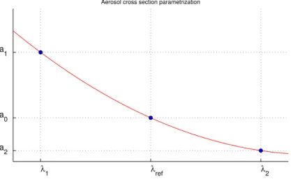
Here we consider four different aerosol cross section models: the standard

(oper-20

ational) 1/λ model (model 1), a second degree polynomial on λ (model 2), 1/λ2 de-pendence (model 3), and a second degree polynomial on 1/λ(model 4). The aerosol models are parametrized using the aerosol extinction at 500 nm (models 1 and 2) or at 300, 500 and 600 nm (models 3 and 4), see Fig. 2. A positivity prior constrains these values. We concentrate on inverting the integrated line densities from the transmission

25

(15)

ACPD

8, 10791–10816, 2008

Title Page

Tables Figures

◭ ◮

Back Close

Full Screen / Esc

Interactive Discussion called vertical inversion of transforming the line densities to the actual constituent

den-sities is a linear operation that is done after the line denden-sities for all the heights have been inverted and is not considered here.

Let N be the vector of integrated line densities of the constituents to be retrieved (O₃, NO₂, NO₃, air, aerosols) and matrix α the corresponding cross sections. The

5

cross section of aerosol depends on the model parametersη(k). The forward model for the observed transmissionT is written as

T(λ, z)= I(λ, z)

I₀(λ) =exp

−α(η(k))N+ǫ(λ),

withǫ(λ)∼N(0, σ_k2w_λ2).

(16)

Here I0(λ) is the spectral intensity measured at a reference height above the atmo-sphere and I(λ, z) is the intensity measured at the tangent heightz. As the chosen

10

aerosol model will affect the size of the residuals, the error variance is assumed to be of formσ_k2w_λ2, with known weightsw_λ for each wavelengthλand model dependent unknown scalarsσ_k2, which are also estimated by the MCMC.

The likelihood function assumes the form

p(T|N, η(k), σ_k2)∝exp − 1

2σ2

k

SS(N, η(k))

!

, (17)

15

whereSS(N, η(k)) is the weighted sum of squares,

SS(N, η(k))=X

λ

  

T(λ)₋expα(η(k))N wλ

  

2

. (18)

As for priors, only positivity constraints for the line densities is used. For the unknown error variance factors,σ_k2, a weakly informative inverse Gamma prior is used (Gamer-man, 1997). All the four models are taken, a priori, to be equally likely. A prior for the

(16)

ACPD

8, 10791–10816, 2008

Title Page

Tables Figures

◭ ◮

Back Close

Full Screen / Esc

Interactive Discussion neutral air would probably help the identification of the aerosol model as the aerosol

and neutral air cross-sections resemble each other and thus produce correlated esti-mates. Note that in the operational GOMOS processing air density is fixed to values provided by European Centre for Medium-Range Weather Forecasts (ECMWF).

5 Results

5

For each line of sight (tangent height), and given one fixed aerosol model, the problem of inverting the line densities from the transmittance is a nonlinear problem with 5 un-knowns. This is a fairly easy problem, assuming we have appropriate initial guesses and the noise level in the transmission spectra is low. The estimation problem can be solved in a least-squares sense as a nonlinear optimization problem using, e.g., the

10

Levenberg-Marquardt method. This is basically the method used in the operational GOMOS algorithm. In this article we use MCMC to replace the operational inversion and take in account the model uncertainty. The MCMC method can also be extended to a one step solution, where all the heights are solved simultaneously, with regulariza-tion (smoothness) priors on the vertical structure of the profiles, see e.g. Haario et al.

15

(2004).

To use the AARJ method for model selection we use the following strategy. Firstly, for each occultation height and for each aerosol model, separate MCMC runs are per-formed using the DRAM method (Haario et al., 2006) to find the individual posterior distributions. From the MCMC chains of these runs the mean vectors and covariance

20

matrices together with their Cholesky factors are calculated to produce the mean vec-torsµ_i, and Cholesky factor matricesR_i,i =1, . . . ,4 needed in the RJMCMC stage. Secondly, an MCMC run is done for a chain of length 50 000 using the AARJ algorithm for further adaptation of the approximations. The resulting chains are visually investi-gated using 1-D plots like those in Fig. 4, in order to judge if the chains have converged.

25

Some automatic convergence criteria could be used as well.

For the model selection, we calculate the relative times the MCMC chain has spent

(17)

ACPD

8, 10791–10816, 2008

Title Page

Tables Figures

◭ ◮

Back Close

Full Screen / Esc

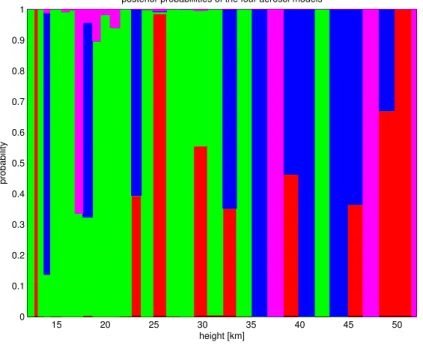
Interactive Discussion in each model. In Fig. 3 the results for each altitude of one GOMOS occultation are

shown. For most of the heights one model stands out as the main candidate, but no single model can be used for all the heights. For altitudes from 14 to 22 km the second order polynomial (Model 2, coloured green) is prevailing. Each of the four models become selected as the most probable one at some of the altitudes. The second

5

order polynomial over 1/λ2(Model 4, magenta) seems to be less favoured. Certainly, a more thorough investigation would be needed to determine the relative merits of different aerosol models for the GOMOS inversion algorithm, but it can already be seen that the choice of the aerosol model can significantly affect the retrievals of the other constituents.

10

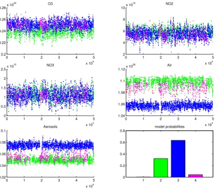
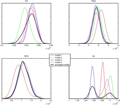
As an illustration of the model averaging we select one altitude at about 18 km where all the four models have gained some posterior probability. Figures 4, 5 and 6 show the MCMC chains, the estimated posterior distributions and the fitted cross-sections for this selected altitude. Model averaging is useful when we are not able to get the best model. The model used for estimation is then a mixture of different models each weighted

ac-15

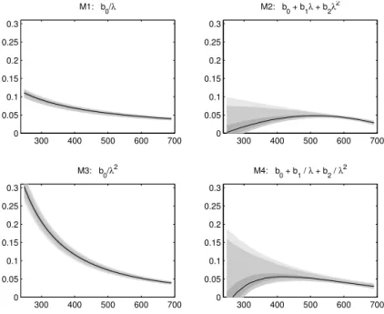
cording to its posterior weight. The uncertainty in the model is taken into account in the predictions and in the posterior inference for the constituents. In Fig. 6 the uncertainty in the cross-section of each model is illustrated. The cross-section curve is calculated for each model parameter in the MCMC chain. Then the corresponding posterior distri-bution for each wavelength is estimated. Together these provide predictive envelopes

20

of the aerosol extinctions. These are drawn as different grey regions in the plots. Figure 5 reveals the effect of the aerosol model on other retrievals. The plots show the marginal posterior distributions of the constituent line densities separately for each model and the posterior distribution of the averaged model. For the retrieval of ozone the difference between posterior mean of Model 2 and of the other models is about

25

(18)

ACPD

8, 10791–10816, 2008

Title Page

Tables Figures

◭ ◮

Back Close

Full Screen / Esc

Interactive Discussion that of the aerosols models. An accurate prior for neutral air, if available, would help

this unidentifiability.

The study of aerosols in the GOMOS inversion is further complicated by the fact that, in addition to aerosols, parts of the unmodelled variations in the GOMOS spectra are due to the scintillation e_ffects caused by turbulence. These e_ffects are actively studied

5

at Finnish Meteorological Institute, and the methods presented in this article will give useful methodological tools for these studies, too.

6 Conclusions

The adaptive automatic RJMCMC method, AARJ, is a novel combination of previous adaptive methodologies that have been found to work reliably in various modelling

ap-10

plications. AARJ provides an easy-to-use adaptive reversible jump MCMC method for Bayesian model selection. It can be used as a tool for automatic model determination and for making simultaneous inference about the model and the model parameters. If one model clearly stands out, we can select it as the “true” model. If the data do not give any definite indication on the right model, and no accurate prior for the model

15

is available, the uncertainty in the modelling can be taken into account in the model predictions by using a weighted mixture of the models. The method itself is a general one and not limited to geophysical applications. It can be used to solve the model se-lection problem for a set of models having different parameters of different dimensions. The new algorithm will make it possible to use Bayesian methods in more realistic

20

modelling settings than before, thus further widening the scope of statistical inversion methodology.

The GOMOS aerosol model selection problem can be successfully studied with the AARJ method. For the GOMOS inversion problem it is natural to consider a set of competing aerosol cross section models, as the most suitable model will depend on

25

the unknown type of aerosols present in the corresponding location. In the present example the number of aerosol cross-section models is four, but the method could

(19)

ACPD

8, 10791–10816, 2008

Title Page

Tables Figures

◭ ◮

Back Close

Full Screen / Esc

Interactive Discussion as well be used to study a larger number of models. The current operational GOMOS

algorithm uses a fixed aerosol model. It would be advisable to further study the effect of the chosen aerosol model of the retrieval of various gas constituents. Different aerosol models could be used depending on the location.

This model selection technique can be used in different applications. The inversion

5

algorithm of the OMI ozone instrument onboard EOS-Aura satellite, for example, has five main aerosol models, each having several sub models (Veihelmann et al., 2007). In the OMI inversion the aerosol model is chosen from a few (2–3) pre-selected models according to the minimumχ2 statistic criteria. Both the GOMOS and OMI inversions could benefit from the model averaging approach that takes into account the

uncer-10

tainty in the model selection.

Acknowledgements. This work is done under financial support from Finnish Funding Agency

for Technology and Innovation (Tekes) within the project MASI – Modelling and Simulation.

References

Bertaux, J. L., Kyr ¨ol ¨a, E., and Wehr, T.: Stellar Occultation Technique for Atmospheric Ozone

15

Monitoring: GOMOS on Envisat, Earth Observation Quarterly, 67, 17–20, 2000. 10804 ESA 2007: GOMOS Product Handbook Issue 3.0, European Space Agency, http://envisat.esa.

int/dataproducts/, 2007. 10793

Gamerman, D.: Markov Chain Monte Carlo – Stochastic simulation for Bayesian inference, Chapman & Hall, 1997. 10798, 10805

20

Green, P. J.: Reversible jump Markov chain Monte Carlo computation and Bayesian model determination, Biometrika, 82, 711–732, 1995. 10799

Green, P. J.: Trans-dimensional Markov chain Monte Carlo, in: Highly Structured Stochastic Systems, edited by: Green, P. J., Hjort, N. L., and Richardson, S., 27, in Oxford Statistical Science Series, Oxford University Press, 179–198, 2003. 10799, 10801

25

Haario, H., Saksman, E., and Tamminen, J.: An adaptive Metropolis algorithm, Bernoulli, 7, 223–242, 2001. 10802

(20)

ACPD

8, 10791–10816, 2008

Title Page

Tables Figures

◭ ◮

Back Close

Full Screen / Esc

Interactive Discussion high dimensional inversion in remote sensing, J. R. Stat. Soc. Ser., Series B, 66, 591–607,

doi:10.1111/j.1467-9868.2004.02053.x, 2004. 10793, 10802, 10806

Haario, H., Laine, M., Mira, A., and Saksman, E.: DRAM: Efficient adaptive MCMC, Statistics and Computing, 16, 339–354, doi:10.1007/s11222-006-9438-0, 2006. 10802, 10803, 10806 Hastie, D.: Towards Automatic Reversible Jump Markov Chain Monte Carlo, Ph.D. thesis,

Uni-5

versity of Bristol Department of Mathematics, 2005. 10803

Kaipio, J. P. and Somersalo, E.: Computational and Statistical Methods for Inverse Problems, Springer, 339 pp., 2004. 10792

Laine, M.: MCMC toolbox for Matlab website, http://www.helsinki.fi/∼_{mjlaine/mcmc/, 2008.} 10804

10

Mira, A.: On Metropolis-Hastings algorithms with delayed rejection, Metron, LIX, 231–241, 2001. 10802

Tamminen, J.: Adaptive Markov chain Monte Carlo algorithms with geophysical applications, Finnish Meteorological Institute Contributions, 47, Finnish Meteorological Institute, Helsinki, 2004. 10793

15

Tamminen, J. and Kyr ¨ol ¨a, E.: Bayesian solution for nonlinear and non-Gaussian inverse prob-lem by Markov chain Monte Carlo method, J. Geophys. Res., 106, 14 377–14 390, 2001. 10793

Vanhellemont, F., Fussen, D., Dodion, J., Bingen, C., and Mateshvili, N.: Choosing a suitable analytical model for aerosol extinction spectra in the retrieval of UV/visible satellite occultation

20

measurements, J. Geophys. Res., 111, 2006. 10804

Veihelmann, B., Levelt, P. F., Stammes, P., and Veefkind, J. P.: Simulation study of aerosol in-formation content in OMI spectral reflectance measurements, Atmos. Chem. Phys., 7, 3115– 3127, 2007, http://www.atmos-chem-phys.net/7/3115/2007/. 10809

(21)

ACPD

8, 10791–10816, 2008

Title Page

Tables Figures

◭ ◮

Back Close

Full Screen / Esc

Model 1 Model 2

95% contour of the target Gaussian approximation

Model 3

target density Gaussian approximation

(22)

ACPD

8, 10791–10816, 2008

Title Page

Tables Figures

◭ ◮

Back Close

Full Screen / Esc

λ₁ λ_ref λ₂

a

1

a

0

a

2

Aerosol cross section parametrization

Fig. 2. Aerosol model parametrization. Each model is parametrised in such way that the parameters correspond to aerosol extinction at one selected wavelength, 300, 500 and 600 nm for three parameter models and 500 nm for one parameter model. This way we can also require positivity for these values and assure that the resulting estimates provide physically meaningful values.

(23)

ACPD

8, 10791–10816, 2008

Title Page

Tables Figures

◭ ◮

Back Close

Full Screen / Esc

15 20 25 30 35 40 45 50

0 0.1 0.2 0.3 0.4 0.5 0.6 0.7 0.8 0.9 1

height [km]

probability

posterior probabiliities of the four aerosol models

(24)

ACPD

8, 10791–10816, 2008

Title Page

Tables Figures

◭ ◮

Back Close

Full Screen / Esc

0 1 2 3 4 5

x 104 3.2

3.22 3.24 3.26 3.28x 10

20 _O3

0 1 2 3 4 5

x 104 2

4 6 8 10x 10

16 _NO2

0 1 2 3 4 5

x 104 0

0.5 1 1.5 2 2.5x 10

15 _NO3

0 1 2 3 4 5

x 104 1.04

1.06 1.08 1.1 1.12x 10

26 _Air

0 1 2 3 4 5

x 104

0.02 0.04 0.06 0.08 0.1

Aerosols

1 2 3 4

0 0.2 0.4 0.6 0.8

model probabilities

Fig. 4. The MCMC chains for the line densities for one selected GOMOS occultation. The horizontal axis runs with the simulation indexes, vertical axis being the simulated and accepted values for the line density for each constituent. The color indicates in witch model the algo-rithm is in each step. Plot on the lower left corner labeled “Aerosol” show the relative aerosol extinction at 500 nm for all models. The last plot shows relative times spent in each model. Of the total 50 000 MCMC simulations of this particular run the models 1, 2, 3 and 4 are visited 129, 16 035, 31 679 and 2157 times, which makes the corresponding marginal model posterior probabilitiesp(k_i_|y),i=1, . . . ,4 to be 0.003, 0.321, 0.634, and 0.043.

(25)

ACPD

8, 10791–10816, 2008

Title Page

Tables Figures

◭ ◮

Back Close

Full Screen / Esc

3.2 3.22 3.24 3.26 3.28

x 1020 O3

0 2 4 6 8 10

x 1016 NO2

0 0.5 1 1.5 2 2.5

x 1015 NO3

1 1.02 1.04 1.06 1.08 1.1 1.12

x 1026 Air

model 1 model 2 model 3 model 4 averaged model

Fig. 5. Marginal posterior density estimates of the constituent line densities calculated from the MCMC chains of Fig. 4. The thicker line is the uncertainty coming from the averaged model that takes into account the model uncertainty. The posterior probabilities of the models are the relative times the chain has spent on each model. This depend on given prior weights for each model and on how well each different model fit the data compared to other models. In the present example, all the models are taken a priori to be equally likely , so p(k)=1/4 for

(26)

ACPD

8, 10791–10816, 2008

Title Page

Tables Figures

◭ ◮

Back Close

Full Screen / Esc

300 400 500 600 700

0 0.05 0.1 0.15 0.2 0.25 0.3

M1: b 0/λ

300 400 500 600 700

0 0.05 0.1 0.15 0.2 0.25 0.3

M2: b

0 + b1λ + b2λ 2

300 400 500 600 700

0 0.05 0.1 0.15 0.2 0.25 0.3

M3: b₀/λ2

300 400 500 600 700

0 0.05 0.1 0.15 0.2 0.25 0.3

M4: b₀ + b₁ / λ + b₂ / λ2

Fig. 6. Estimated aerosol extinctions for the selected altitude of the example given in the text. Solid line is the fitted median cross section. Grey areas correspond to 50%, 95% and 95% posterior limits of the extinctions. The model are the following. Model 1: linear for 1/λ, Model 2: a second degree polynomial onλ, Model 3: linear for 1/λ2, Model 4: a second degree polynomial on 1/λ.