ISSN 0104-6632 Printed in Brazil
www.abeq.org.br/bjche
Vol. 30, No. 03, pp. 619 - 625, July - September, 2013
Brazilian Journal
of Chemical
Engineering
FLOW OF A WILLIAMSON FLUID OVER
A STRETCHING SHEET
S. Nadeem
1*, S. T. Hussain
1and Changhoon Lee
21
Department of Mathematics, Quaid-I-Azam University 45320, Phone: + 92 51 90642182, Islamabad 44000, Pakistan.
E-mail: [email protected] 2
Department of Computational Science and Engineering, Yonsei University, Seoul, Korea.
(Submitted: January 26, 2012 ; Revised: May 9, 2012 ; Accepted: June 10, 2012)
Abstract - In the present article, we have examined the two dimensional flow of Williamson fluid model over a stretching sheet. The governing equations of pseudoplastic Williamson fluid are modelled and then simplified by using similarity transformations and boundary layer approach. The reduced equations are then solved analytically with the help of homotopy analysis method. The physical features of the model are presented and discussed through graphs.
Keywords: Williamson fluid; Stretching sheet; Homotopy analysis method.
INTRODUCTION
In non-Newtonian fluids, the most commonly encountered fluids are pseudoplastic fluids. The study of the boundary layer flow of pseudoplastic fluids is of great interest due to its wide range of application in industry such as extrusion of polymer sheets, emulsion coated sheets like photographic films, solutions and melts of high molecular weight polymers, etc. The Navier Stokes equations alone are insufficient to explain the rheological properties of fluids. Therefore, rheological models have been proposed to overcome this deficiency. To explain the behaviour of pseudoplastic fluids many models have been proposed like the power law model, Carreaus model, Cross model and Ellis model, but little attention has been paid to the Williamson fluid model. Williamson (1929) discussed the flow of pseudoplastic materials and proposed a model equation to describe the flow of pseudoplastic fluids and experimentally verified the results. Lyubimov and Perminov (2002) discussed the flow of a thin layer of a Williamson fluid over an inclined surface
in the presence of a gravitational field. Dapra and Scarpi (2007) developed the perturbation solution for a Williamson fluid injected into a rock fracture. Peristaltic flow of a Williamson fluid has been discussed by Nadeem et al. (2010). Vasudev et al. (2010) studied the peristaltic pumping of a Williamson fluid through a porous medium considering heat transfer. Cramer et al. (1968) showed that this model fits the experimental data of polymer solutions and particle suspensions better than other models. For pseudoplastic fluids the power law model predicts that the apparent/effective viscosity should decrease indefinitely with increasing shear rate, which means infinite viscosity at rest and zero viscosity as the shear rate approaches infinity. A real fluid has both minimum and maximum effective viscosities depending upon the molecular structure of the fluid. In the Williamson fluid model, both the minimum (μ∞) and maximum viscosities (μ0) are considered. So, for pseudoplastic fluids (for which the apparent viscosity does not go to zero at infinity), it will give better results.
considered the boundary layer flow of a Williamson fluid over a stretching sheet. Stretching sheet flows are of great importance in many engineering applica-tions like extrusion of a polymer sheet from the die, the boundary layer in liquid film condensation processes, emulsion coating on photographic films, etc. Sakiadis (1961) initiated the study of boundary layer flows over a continuous surface and formulated the two dimensional boundary layer equations. Tsou et al. (1967) extended the work of Sakiadis and considered the heat transfer in the boundary layer flow over a continuous surface and experimentally verified Sakiadis’ results. Erickson et al. (1966) included the heat and mass transfer on a stretching surface with suction or injection. Many researchers later investigated boundary layer flow over a stretching surface, such as Gupta and Gupta (1977), Ishak (2008), and Nadeem (2010).
The objective of the present paper is to present the modelling of a two-dimensional Williamson fluid for a stretching sheet. The highly non-linear partial differential equations are simplified by using suitable similarity transformations and the resulting reduced equations are then solved analytically with the help of homotopy analysis method (HAM) (see Liao, 2003, 2004). The results are discussed through graphs for various physical parameters of interest. The coefficient of skin friction, shear stress and apparent viscosity are also plotted.
FLUID MODEL
For an incompressible Williamson fluid, the continuity and momentum equations are given as:
divV=0, (1)
d
div ,
dt
ρ V = S+ρb (2)
where ρ is the density, V is the velocity vector, S
is the Cauchy stress tensor, b represents the specific body force vector and d / dt represents the material time derivative. The constitutive equations of the Williamson fluid model are given as:
p ,
= − +
S I τ (3)
0
1
( )
[ ] ,
1 ∞
∞ μ −μ
μ + − Γγ A
τ = (4)
in which p is the pressure, I is the identity vector,
τ is the extra stress tensor, μ0 and μ∞ are the limiting viscosities at zero and at infinite shear rate,
0
Γ > is the time constant, A1 is the first Rivlin-Erickson tensor and γ is defined as follows
2 1
1 , 2
trace( ), γ = π
π A
= (5)
2 2 2 1/2
u 1 u v v
[( ) ( ) ( ) ] ,
x 2 y x y
∂ ∂ ∂ ∂
γ = ∂ + ∂ +∂ + ∂
(6)
where π is the second invariant strain tensor. Here we have only considered the case for which μ =∞ 0 and 1.Γγ < Thus, the extra stress tensor takes the form:
0 1
[ ] ,
1 μ − Γγ A
τ = (7)
or, by using binomial expansion, we get:
0[1 ] 1,
μ + Γγ A
τ = (8)
The components of the extra stress tensor are:
xx 0
xy yx 0
yy 0
xz yz zx zy zz
u
2 [1 ] ,
x
u v
[1 ]( ),
y x
v
2 [1 ] ,
y
0. ∂
τ = μ + Γγ ∂
∂ ∂
τ = τ = μ + Γγ ∂ +∂
∂ τ = μ + Γγ ∂
τ = τ = τ = τ = τ =
(9)
Mathematical Formulation
Let us consider a steady, two-dimensional flow of an incompressible Williamson fluid over a wall coinciding with the plane y=0, the flow being confined to y>0. Two equal and opposite forces are applied along the x -axis to produce stretching, keeping the origin fixed. The flow is generated due to the linear stretching. In the absence of a body force, the governing equations in component form can be defined as:
u v
0,
x y
∂ +∂ =
where u(x, y) and v(x, y) are the velocity components along the flow direction and normal to the flow direction, respectively:
xy xx
u u p
(u v ) ,
x y x x y
∂τ
∂ ∂ ∂ ∂τ
ρ ∂ + ∂ = −∂ + ∂ + ∂ (11)
yx yy
v v p
(u v ) ,
x y y x y
∂τ ∂τ
∂ ∂ ∂
ρ + = − + +
∂ ∂ ∂ ∂ ∂ (12)
where τ τ τxx, xy, yy are the components of the extra stress tensor Eq. (7). Applying the boundary layer approximations to the components of the tensor, where the order of x and u is 1 while the order of
,
Γ y and v is .δ
2 2 1/2
2
1
[1 { 1 1} ]
δ δ δ
δ
2
xx 0
2 2 1/2
u u u
( )
x x x
2
,
1 u v v
( ) ( )
2 y x y
{
}
⎧ ∂ + Γ∂ ∂ ⎫
⎪ ∂ ∂ ∂ ⎪
τ = μ ⎪⎨ ⎪⎬
ρ ρ ⎪ ∂ ∂ ∂ ⎪
+ + +
⎪ ∂ ∂ ∂ ⎪
⎩ ⎭
(13)
2 2 1/2
2
1 1
[1 { 1 1 } ] ( )
δ δ δ δ δ
δ
xy 0 1 ( u)2 1( u v)2 ( v)2 1/2
x 2 y x y
u v
( ).
y x
[
{
} ]
τ =μ + Γ ∂ + ∂ ∂+ + ∂
ρ ρ ∂ ∂ ∂ ∂
∂ ∂+ ∂ ∂
(14)
Each term of Eq. (11) and Eq. (12) must be of order 1 . So we retained those terms of Eq. (13) and Eq. (14) that have order 1 and δ, respectively. In the absence of a pressure gradient, we finally arrive at:
2 2
2 2
u u u u u
u v 2 .
x y y y y
∂ + ∂ = ν∂ + νΓ∂ ∂
∂ ∂ ∂ ∂ ∂ (15)
The corresponding boundary conditions are:
w
u U Bx; v 0 at y 0,
u 0 as y ,
= = = =
→ → ∞ (16)
where ν is the kinematic viscosity, U is the velocity w
at the wall and B>0 is the stretching parameter. Introducing the following transformations:
( )
( )
B u=Bxf′ η , v= − ν η η =B f , y.ν (17)
Making use of transformations (17), Eq. (15) takes the form:
2
f′′′ ′− +f ff′′+ λf f′′ ′′′=0, (18)
with the corresponding boundary conditions:
f 0,f 1 at 0,
f 0 as ,
′
= = η =
′ → η → ∞ (19)
where λ, the dimensionless Williamson parameter. is defined as:
3
2B
x .
λ = Γ
ν (20)
For λ =0, Eq. (18) reduces to the classical boundary layer equation for a viscous flow. Physical quantities of interest are the wall shear stress τw and the coefficient of skin friction c . After using boundary f layer approximations, τw is given by:
2
w 0
y 0
u u
[ ( ) ] ,
y 2 y =
∂ Γ ∂
τ = μ ∂ + ∂ (21)
The coefficient of skin friction is defined as:
w
f 2
w
c .
U τ =
ρ (22)
In dimensionless form it is defined as:
2 f
0
Rec (f f ) ,
2 η=
λ ⎡ ′′ ′′ ⎤
=⎢ + ⎥
⎣ ⎦ (23)
where Re= Bx /2 ν is the Reynolds number.
Homotopy Analysis Solutions
We choose the set of base functions:
{
k}
exp( n ), k 0, n 0 ,
and can write:
0 k k
0,0 m, n
n 0 k 0
f ( ) a a exp( n ),
∞ ∞
= =
η = +
∑∑
η − η (25)where akm, n is the coefficient. With the help of boundary conditions (19), the initial approximation and auxiliary linear operator are chosen as:
0
f ( )η = −1 exp(−η), (26)
3
f 3
d f df
L (f ) ,
d d
= −
η
η (27)
f 1 2 3
L [C +C exp( )η +C exp(−η =)] 0, (28)
and C i
(
i= −1 3)
are the arbitrary constants.Zeroth Order Deformation Equation
If q∈[0,1] is the embedding parameter and the non-zero auxiliary parameter is ħ, then the problem at the zeroth order deformation is:
f 0 f
(1 q)L [f ( ;q) f ( )]− η − η =q N [f ( ;q)],= η (29)
(
)
00
f ( ;q)
f ( ;q) 0, 1,
f ( ;q)
0, η=
η=
η→∞ ⎛∂ η ⎞
η = ⎜ ⎟ =
∂η
⎝ ⎠
⎛∂ η ⎞ = ⎜ ∂η ⎟
⎝ ⎠
(30)
where the nonlinear operator is defined as:
2 3
f 3
2 2
2 3
2 3
f ( ;q) f ( ;q) N [f ( ;q)]
f ( ;q) f ( ;q)
( f ( ;q)) ( f ( ;q)) ,
( ) ( )
⎛ ⎞
∂ η ∂ η
η = − ⎜ ∂η ⎟
∂η ⎝ ⎠
∂ η + η
∂η
⎛⎛ ∂ η ⎞⎛ ∂ η ⎞⎞ + λ⎜⎜⎜⎜ ∂η ⎟⎜⎟⎜ ∂η ⎟⎟⎟⎟
⎝ ⎠⎝ ⎠
⎝ ⎠
(31)
When q=0 and q=1, then:
0
f ( ;0)η = ηf ( ), f ( ;1)η = ηf ( ). (32)
With the help of a Taylor series expansion:
m
0 m
m 1
f ( ;q) f ( ) f ( )q , ∞
=
η = η +
∑
η (33)m
m m
q 0
1 f ( ;q)
f ( ) ,
m! q =
∂ η
η =
∂ (34)
the auxiliary parameter is chosen in such a way that Eq. (33) converges at q=1; thus
0 m
m 1
f ( ) f ( ) f ( ), ∞
=
η = η +
∑
η (35)mth Order Deformation Equations
The m order approximation is defined as: th
f
f m m m 1 m
L [f ( )η − χ f − ( )]η ==R ( ),η (36)
m m m
f (0)=f (0)′ =f ( )′ ∞ =0, (37)
where:
m 1 f
m m 1 m 1 k k m 1 k k
k 0 m 1
m 1 k k l k 0
R ( ) f [f f f f ]
f f ,
−
′′′ ′′ ′ ′
− − − − −
= −
′′ ′′′ − − − =
η = + − +
λ
∑
∑
(38)
m
0, m 1, . 1, m 1
≤ ⎧ χ = ⎨ >
⎩ (39)
The general solution for Eq. (36) is defined as:
m m 1 2 3
f ( )η =f ( ) C∗ η + +C exp( ) C exp(η + −η), (40)
where f ( )m∗ η is a special function. We can determine constants using conditions (37) :
m
2 3 1 3 m
0
f ( )
C 0, C ,C C f (0).
∗
∗
η= ∂ η
= = ∂η = − − (41)
RESULTS AND DISCUSSION
We know that the convergence of the solution of Eq. (33) depends upon the non-zero auxiliary parameter ħ. To obtain an admissible value of ħ, the
ħ-curve is plotted for the 20 order of approximation. th In Fig. (1), it can be observed that the admissible range of ħ is 1.5− ≤ ≤ −= 0.5. In order to choose the best value of ħ , the residual error in f is plotted for different values of ħ (see Fig. (2)). It is observed that we can choose any value between 1.4− ≤ ≤ −= 0.9. It can be seen from Table 1 that convergence of the HAM solution is obtained at the 5 order of approximation. th
Figure 1: = -curve of f''(0)
Figure 2: Residual error in f at η=0
Table 1: Convergence of the HAM solution for different order of approximation when λ= 0.1.
Order of approximation -f (0)′′
1 1.04
5 1.03446 6 1.03446 10 1.03446 15 1.03446
Fig. (3) plots the non-dimensional velocity f′ against η for various values of the Williamson fluid
parameter λ. It is observed that, with the increase in λ, the velocity field and boundary layer thickness decrease. Fig. 4 shows that f decreases with an increase in .λ When we increase the value of Γ or B (keeping the other parameters fixed), it results in an increase in λ. So the velocity profile as well as the boundary layer thickness decrease with an increase in Γ or B . Table 2 shows the effects of λ on the skin friction coefficient at ħ=-1.2. It also depicts that, with the increase of λ, the magnitude of the coefficient of skin friction decreases (see Fig. 5). In Figs. 6(a) and 6(b), the shear stress and apparent viscosity for the Williamson fluid are plotted against the deformation rate. These figures show that the behaviour is quite similar to pseudoplastic fluids.
1 2 3 4 5 6
0 1.0
0.8
0.6
0.4
0.2
0.0
η
f (′ )η
1.2 = −
=
1 2 3 4 5 6
0 1.0
0.8
0.6
0.4
0.2
0.0
1 2 3 4 5 6
0 1 2 3 4 5 6
0 1.0
0.8
0.6
0.4
0.2
0.0 1.0
0.8
0.6
0.4
0.2
0.0
η
f (′ )η
1.2 = −
=
Figure 3: Variation of f' for various values of λ
1 2 3 4 5 6
0 1.0
0.8
0.6
0.4
0.2
0.0
η f(η)
1.2 = −
=
1 2 3 4 5 6
0 1.0
0.8
0.6
0.4
0.2
0.0
1 2 3 4 5 6
0 1 2 3 4 5 6
0 1.0
0.8
0.6
0.4
0.2
0.0 1.0
0.8
0.6
0.4
0.2
0.0
η f(η)
1.2 = −
=
Figure 4: Variation of f for various values of λ
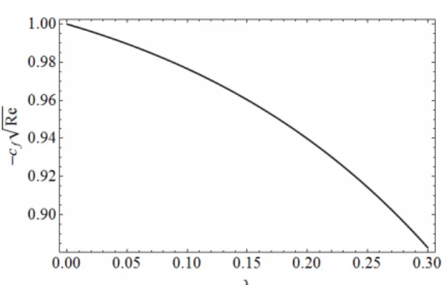
Table 2: Values of the coefficient of skin friction for different values of λ.
λ - Recf
Figure 5: Variation of the coefficient of skin friction for different values of λ
(a)
Figure 6(a): Shear stress against deformation rate when λ =0.4
(b)
Figure 6(b): Apparent viscosity against deformation rate when λ =0.4
CONCLUDING REMARKS
We have investigated the boundary layer flow of a Williamson fluid over a stretching surface. The
nonlinear differential equation is solved analytically by using HAM. At the end we can conclude that:
1. f′ decreases with an increase in the Williamson parameter .λ
2. The coefficient of skin friction decreases parabolically with an increase in .λ
3. The Williamson fluid model describes the flow of pseudoplastic fluids.
ACKNOWLEDGEMENT
This research was supported by the WCU (World Class University) program through the National Research Foundation of Korea (NRF) funded by the Ministry of Education, Science and Technology R31-2008-000-10049-0.
REFERENCES
Abbasbandy, S., The application of homotopy analysis method to solve a generalized Hirota-Satsuma coupled KdV equation. Physics Letters A, 361, No. 6, 478 (2007).
Abbasbandy, S., Homotopy analysis method for heat radiation equations. International Communications in Heat and Mass Transfer, 34, No. 3, 380 (2007). Abbasbandy, S., The application of homotopy
analysis method to nonlinear equations arising in heat transfer. Physics Letters A, 360, No. 1, 109 (2006).
Abbasbandy, S. and Shirzadi, A., A new application of the homotopy analysis method: Solving the Sturm--Liouville problems. Communications in Nonlinear Science and Numerical Simulation, 16, No. 1, 112 (2011).
Cramer, S. D. and Marchello, J. M., Numerical evaluation of models describing non-Newtonian behavior. American Institute of Chemical Engineers Journal, 14, 980 (1968).
Dapra and Scarpi, G., Perturbation solution for pulsatile flow of a non-Newtonian Williamson fluid in a rock fracture. International Journal of Rock Mechanics and Mining Sciences, 44, 271 (2007).
Erickson, L. E., Fan, L. T. and Fox, V. G., Heat and mass transfer in the laminar boundary layer flow of a moving flat surface with constant surface velocity and temperature focusing on the effects of suction/injection. Industrial & Engineering Chemistry Research, 5, 19 (1966).
flow in a third-grade fluid with variable viscosity. Mathematical and Computer Modelling, 52, No. 9-10, 1783 (2010).
Ellahi, R., Effects of the slip boundary condition on non-Newtonian flows in a channel. Communications in Nonlinear Science and Numerical Simulation, 14, No. 4, 1377 (2009).
Ellahi, R. and Afzal, S., Effects of variable viscosity in a third grade fluid with porous medium: An analytic solution. Communications in Nonlinear Science and Numerical Simulation, 14, No. 5, 2056 (2009).
Ellahi, R., Raza, M. and Vafai, K., series solutions of non-Newtonian nanofluids with Reynolds model and Vogels model by means of the homotopy analysis method, Mathematical and Computer Modelling, 55, No. 7, 1876 (2012).
Gupta, P. S. and Gupta, A. S., Heat and mass transfer on a stretching sheet with suction or blowing. Canadian Journal of Chemical Engineering, 55, No. 6, 744 (1977).
Ishak, A., Nazar, R. and Pop, I., Heat Transfer over a stretching surface with variable heat flux in micropolar fluids. Physics Letters A, 372, No. 5, 559 (2008).
Lyubimov, D. V. and Perminov, A. V., Motion of a thin oblique layer of a pseudoplastic fluid. Journal of Engineering Physics and Thermophysics, 75, No. 4, 920 (2002).
Liao, S., Beyond Perturbation: Introduction to the Homotopy Analysis Method. Chapman & Hall/ CRC, Boca Raton (2003).
Liao, S., On the analytic solution of magneto hydrodynamic flows of non-Newtonian fluid over a stretching sheet. Fluid Mechanics, 488, 189 (2003).
Liao, S., A new branch of solutions of unsteady boundary layer flow over an impermeable stretched plate. International Journal of Heat and Mass Transfer, 48, 2529 (2005).
Liao, S., On the homotopy analysis method for nonlinear problems. Applied Mathematics and Computation, 147, 499 (2004).
Nadeem, S. and Akram, S., Influence of inclined magnetic field on peristaltic flow of a Williamson fluid model in an inclined symmetric or asymmetric channel. Mathematical and Computer
Modelling, 52, 107 (2010).
Nadeem, S. and Akbar, N. S., Numerical solutions of peristaltic flow of Williamson fluid with radially varying MHD in an endoscope. International Journal for Numerical Methods in Fluids, 66, No. 2, 212 (2010).
Nadeem, S. and Akram, S., Peristaltic flow of a Williamson fluid in an asymmetric channel. Communications in Nonlinear Science and Numerical Simulation, 15, 1705 (2010).
Nadeem, S., Hussain, A. and Khan, M., HAM solutions for boundary layer flow in the region of the stagnation point towards a stretching sheet. Communications in Nonlinear Science and Numerical Simulation, 15, No. 3, 475 (2010). Nadeem, S., Hayat, T., Abbasbandy, S. and Ali, M.,
Effects of partial slip on a fourth-grade fluid with variable viscosity: An analytic solution. Nonlinear Analysis: Real World Applications, 11, No. 2, 856 (2010).
Nadeem, S., Hussain, A. and Vajravelu, K., Effects of heat transfer on the stagnation flow of a third order fluid over a shrinking sheet. Zeitschrift für Naturforschung A, 65, 969 (2010).
Nadeem, S., Hussain, A., Malik, M. Y. and Hayat, T., Series solutions for the stagnation flow of a second-grade fluid over shrinking sheet. Applied Mathematics and Mechanics, 30, 1255 (2009). Nadeem, S. and Hussain, A., MHD flow of a viscous
fluid on a nonlinear porous shrinking sheet with homotopy analysis method. Applied Mathematics and Mechanics, 30, No.12, 1569 (2009).
Sakiadis, B. C., Boundary layer behavior on continuous solid flat surfaces. American Institute of Chemical Engineers Journal, 7, 26 (1961). Tsou, F. K., Sparrow, E. M. and Goldstein, R. J.,
Flow And heat transfer in the boundary layer on a continuous moving surface. International Journal of Heat and Mass Transfer, 10, 219 (1967). Vasudev, C., Rao, U. R., Reddy, M. V. S. and Rao,
G. P., Peristaltic pumping of Williamson fluid through a porous medium in a horizontal channel with heat transfer. American Journal of Scientific and Industrial Research, 1, No. 3, 656 (2010). Williamson, R. V., The flow of pseudoplastic