Condition Monitoring
S. S. Lampreia1,∗, J. G. Requeijo2, J. M. Dias2and V. Vairinhos1,3
1Naval Academy – Mechanical Engineer Department, CINAV – Centro de Investigac¸˜ao Naval
2Faculty of Science and Technology of the Universidade Nova of Lisbon,
Mechanical and Industrial Engineer Department
[email protected], [email protected]
3CENTEC – Center of Naval Engineering and Technology of Instituto Superior
T´ecnico-Universidade T´ecnica of Lisbon
Abstract
The progressive degradation of presently operating electro-mechanical systems is a certain future fact. To minimize losses, maintenance costs and eventual replacements, condition monitoring should be applied to critical equipment (Condition Based Maintenance – CBM). The state of equipment can be predicted at any moment using statistical methods to analyze condition monitoring data. In this paper, collected data are vibration values, obtained atppoints (p=4 for instance) of an experimental equip-ment, formingpvariables. When independence condition does not hold, it is suggested modeling data with Auto-Regressive Integrated Moving Average (ARIMA) models, and using the residues of the esti-mated model for Phase I. In Phase I, the estimation of parameters is achieved using the HotellingT2
control chart; only after applying the defined ARIMA model, thepvariables are treated. In Phase II, equipment state is artificially degraded through induced failures and failure prediction obtained using special multivariate control charts for data statistical treatment. Assuming data independence and normality, Multivariate Exponentially Weighted Moving Average Modified (MEWMAM) control charts are applied in Phase II to data collected from an electric pump, controlling the behavior of data using this procedure. In Phase II, for non-independent data the prediction errors from the adjusted model are used instead of original data. To show that the suggested methodology can be applied to propulsion systems, simulated data from a gas turbine are used. Using these methodologies it is possible to run online condition monitoring, and act in time, to minimize maintenance costs and maximize equipment performance.
Keywords:Condition monitoring, Vibration detection and analysis, Statistical process control, Multivariate Exponential Weighted Moving Average (MEWMA) control chart
Acronyms
AL Alert Level AR Auto-regressive
AR2 Auto-regressive of order 2
ARIMA Auto-regressive integrated Moving Average
ARMA Mix of AR and MA
ACF Auto-correlation Function
ARL Average Run Length
CBM Condition Based Maintenance
CL Center Line
CUSUM Cumulative Sum
EWMA Exponentially Weighted Moving Average
EWMAM Exponentially Weighted Moving Average Modified EACF Estimated Auto-correlation Function
EPACF Estimated Partial Auto-correlation Function
GG Gas Generator
k Observation instant for the 4 variables
k Safety Factor forTLcalculus
K Upper Control Level in MEWMAM Control Chart
K1 Alert Level in MEWMAM Control Chart
kW kilo Watt
MA Moving Average
MEWMA Multivariate Exponentially Weighted Moving Average
MEWMAM Multivariate Exponentially Weighted Moving Average Modified PACF Partial Auto-correlation Function
PT Power Turbine
SPC Statistical Process Control
rpm Rotation Per Minute
T2 Hotelling Control Chart, or Multivariate Traditional Control Chart
T2M Hotelling Modified Control Chart, or Multivariate Traditional Modified Control Chart
(TL)N Limit Defined by Normative or the manufacturer
UCL Upper Control Level
1
Introduction
When implementing a condition based maintenance system, the type and equipment performance must be considered. The main targets are to reduce maintenance costs and optimize operation.
Statistical methods are applied to condition estimation, the main objectives being to categorize anomalies, identify components involved in those anomalies, estimate possible trends and predict the time to failure[1].
To decide which features to measure, those that best represent the equipment behavior must be chosen. For rotating equipment, vibrations, oil analysis, and thermography are the most representative of its states[2]; these methods are suggested since no intervention is needed as part of the data collection task. For the present study, vibration measurement was the selected method and a portable vibration collector was used, the uploading of data being controlled using the equipment software. To define the vibration parameters and monitoring, Statistical Process Control (SPC) with some modifications was applied.
2
Control Charts
Given the right conditions, multivariate control charts can be applied for process control. In this work HotellingT2control chart was used for equipment monitoring in Phase I, both to check the equipment stability and to define its parameters; the MEWMAM control chart was used for the monitoring in Phase II.
2.1 Phase I –TTT222traditional control charts
The design ofT2control charts obey some rules, the first one being that more than one variable should be observed, and then enough data should be collected to estimate the process parameters. Given the data specifications, individual observations(n=1)control charts will be used[3].
2.1.1 Independent data
If the observedpvariables in control are independent, a suitable model isXij =µj+εij, whereXij
is the observationifor variablej, µj is the process mean for the variablej, εijare iid normal random
variables with mean zero and standard deviationσε(white noise).
In Phase I, withmindividual observations at each point,Xij(i=1, . . . , m;j =1, . . . , p), the mean,
(X¯j), the varianceSij, and the covarianceSj hare calculated for each point and each pair of points. The
vector mean(X)¯ and the covariance matrix(S)are given by the next expressions[4]:
¯
X=(X¯1,X¯2, . . . ,X¯p)T S= ⎡ ⎢ ⎢ ⎢ ⎢ ⎢ ⎢ ⎢ ⎢ ⎣
S11 S12 S13 . . . S1p
S21 S22 S23 . . . S2p · · · . . . · · · · . . . · · · · . . . ·
Sp1 Sp2 Sp3 . . . Spp ⎤ ⎥ ⎥ ⎥ ⎥ ⎥ ⎥ ⎥ ⎥ ⎦ (1)
For each observation instantktheT2control charts are based on the statistic given by (2):
(T2)k =(Xk− ¯X)TS−1(Xk− ¯X), (k=1,2. . . p) (2)
Table 1 T2control chart limits
Chart CL UCL
Phase I 0 (m−m1)2βα;p/2;(m−p−1)/2
2.1.2 Auto-correlated data
If a variable has a significant auto-correlation,T2statistic is estimated using the residues from obser-vations; otherwise, the procedure may suggest unnecessary preventive interventions for equipment in good state. The variablesXk,X¯ andSare replaced with the corresponding residues and the mean vector
and covariance residues matrix are built. For correlated observations, data is modeled with an ARIMA
(p, d, q)model[5]and the corresponding residues are obtained, according with the following procedure. The process auto-correlation is analyzed studying the Auto-Correlation Function (ACF) and the partial auto-correlation function (PACF). To identify a suitable model member from family ARIMA(p, d, q), the functions (ACF) and (PACF) are compared using the corresponding estimations: the Estimated Auto-Correlation Function (EACF) and the Estimated Partial Auto-Auto-Correlation Function (EPACF)[6, 7].
A process follows an ARIMA(p, d, q)model when∇dX
t-the orderddifference process-follows an
ARMA (Auto-regressive Moving Average)(p, q)model. The model defined by ARIMA(p, d, q)is:
p(B)∇d=Xt =q(B)εt (3)
p(B)=(1−φ1B−φ2B2− · · · −φpBp) (4)
q(B)=(1−θ1B−θ2B2− · · · −θqBq) (5)
Here p andq are, respectively, symbolic polynomials of order p andq on B. See[4] and[7] for
details. The Backshift operatorBis defined by:
B(Xt)=Xt−1 (6)
and the delta operator by:
∇(Xt)=Xt−Xt−1=(1−B)(Xt) (7)
See[5]and[7]for details.
The residues corresponding to the specified model areet =Xt− ˆXt, whereXˆt is an estimation of the
process expected value for the periodt. TheT2control chart is built using those residues. The process mean is estimated using (8) below when the process is modeled by an AR(p)(Auto-regressive) =
ARIMA(p,0,0)or by a MA(q)(Moving Average)= ARIMA(0,0, q)[7]
E(X)=µ= ξ
1−pj=1φj
E(X)=µ (8)
2.2 Phase II – special control charts – modified MEWMA
Cumulative sum modified control charts (CUMSUM) are chosen instead of traditional control charts, given its sensitivity to small changes.
The EWMA (Exponentially Weighted Moving Average) multivariate modified control chart, MEWMAM, to control the mean is based on theT2statistics[8], defined for instanti, (i=1,2. . . )by:
Ti2=Z′i
−1
Z
where
Zi =RXi +(I−R)Zi−1, Z0=0,
Z
= λ
2−λ(1−(1−λ)
2i)
(10)
In this equation,Iis the identity matrix andR=diag(λ1, λ2, . . . , λp), whereλj(j=1,2, . . . , p)is
a weighting constant for variableXj. Usuallyλ1=λ2= · · · =λp=λ. In this case,Ziand the inverse
matrix, are defined respectively by:
Zi =λXi +(1−λ)Zt−1 −1
(Zi =λXi +(1−λ)Zt−1) (11)
The modification of MEWMA statistics is based, for each variablej, on the maximum acceptable vibration levelTL. This value is calculated as a function of the maximum acceptable vibration level
given by a norm or standard(TL)Standard, the standard deviationσ and a safety factork1, as follows:
(TL)j =((TL)Standard−kσ )j (12)
TL is used instead of the mean; the use of the mean is correct for industrial production, but, for
equipment monitoring it could lead to unnecessary interventions. Since data is auto-correlated and we are applying the MEWMA, the expressions (13) forZi and the inverse matrix will be used. Theei is
the predicted error calculated based on the ARIMA model
Zi =λ(ei−TL)+(1−λ)Zt−1 −1
(λ(ei −TL)+(1−λ)Zt−1) (13)
An out of control situation is detected whenTi2> H, whereHis the control limit. In[8]the values ofHforARLIn Control=200 and forδ(µ)are suggested when:
p=2,4,6,10,15(0,5;1,0;1,5;2,0;3,0) and
λ=(0,05;0,10;0,20;0,30;0,40;0,50;0,60;0,80).
From the same reference optimal values for MEWMA control chart can be obtained, the best values
λandH forp =4,10,20 are forARLIn Control =500, ARLIn Control =1000, for different values of
δ(µ)(0,5;1,0;2,0;3,0)[9].
MEWMAM control chart, like univariate EWMA control chart, shows high sensitivity when compared withT2andχ2, considering small and moderate shifts[8].
3
Methodology
To define the methodology for monitoring data, sample size(m)is a fundamental input for specified statistical procedures.
1. To define the methodology for monitoring data, sample size(m)is a fundamental input for specified statistical procedures.
1Assuming normal distributed data and after some empirical experimentation with confidence interval, we
2. In Phase I, data is checked for independence, comparing the EACF and the EPACF. If data is auto-correlated, the ARIMA model should be applied, and the T2 control chart is calculated for the residues; if not, the original data are used. For normal and stable data distribution, the mean vector and the covariance matrix are calculated. For this Phase, at least 200 samples of individual observations must be taken.
3. In the Phase II the MEWMAM control chart is used to monitor the equipment. In this Phase the equipment is monitored since the first observation, and only under defined rules (see below) preventive actions are taken. To define those rules, the value(TL)Standard described above should be evaluated according to international standards or manufacture’s rules. To define the control chart limits:
• Estimate the two limits to control the mean level of vibration, specifically, the Upper Control Limit and the Alert Value (AL).
• Based on ISO 2372:2003 Standard specify the vibration level at which the system must suffer an intervention.
• Rules to act on the system:
– Execute an intervention to detect any anomalous situation when 8 consecutive points are above the AL.
– Proceed to a maintenance intervention when 5 consecutive points above UCL are observed.
4
Case Study
4.1 Real data prototype
For the case study, vibration data from an electro-pump were used. Four points representing the machine state were selected for the data collection.
To test the MEWMA sensitivity, an anomaly with four state aggravations was forced. In what follows vibration values and Root Mean Square (RMS) are expressed in velocity units (mm/s).
4.1.1 Phase I –TTT222control chart
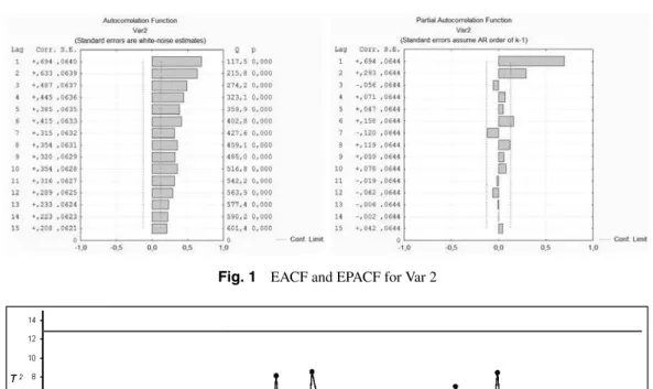
Assuming the electro-pump working properly, for Phase I, the equipment parameters are estimated based on 241 individual observations. The first step is testing the data for independence, comparing ACF with PACF using its estimators EACF and EPACF for the four variables, the result being a model that best fits the data. In the present case, the result is an auto-correlated data set, so we use the residues from the adjusted model in the Shewhart control charts. In this specific case, the residues are studied using the Statistica software. Considering only, for illustrative purposes, the variable Var 2, a point above the UCL was detected, so it was replaced using the defined model. Figure 1 shows the EACF and EPACF for the variable 2, where auto-correlation is significant and we can see a AR2 (Auto-regressive of order 2) ARIMA model, where for ACF we have an exponential decrease after a certain lag order, and for PACF significant peaks through lags log (p) (lag 1 and lag 2).
All the four variables are well fitted with an AR2 ARIMA model; given space limitations we show only values corresponding to Var 2:ξ =0,1025, ϕ1=0.4945 andϕ2=0.2919.
Fig. 1 EACF and EPACF for Var 2
Fig. 2 T2control chart – Phase I
(residues and variables) and covariance matrix are estimated[3]. For graphic reasons, in Fig. 2, only 100 of the 241 samples are shown
¯
e= ⎡
⎢ ⎢ ⎢ ⎣
0,00033 0,00021 0,00034 0,00041
⎤
⎥ ⎥ ⎥ ⎦
¯
X= ⎡
⎢ ⎢ ⎢ ⎣
0,406 0,4810 0,7400 0,5220
⎤
⎥ ⎥ ⎥ ⎦
S= ⎡
⎢ ⎢ ⎢ ⎣
0,000726 −0,000057 0,000137 0,000035
−0,000057 0,000686 −0,000123 −0,000007 0,000137 −0,000123 0,007102 0,000298 0,000035 −0,000007 0,000298 0,001627
⎤
⎥ ⎥ ⎥ ⎦
4.1.2 Phase II – MEWMAM control chart
For Phase II the limit vibration was extracted from the ISO 2372:2003. For an electrical engine with 1.5 kW, 1.12 mm/s (RMS) is the allowable limit of an equipment of class I; let this value be named as
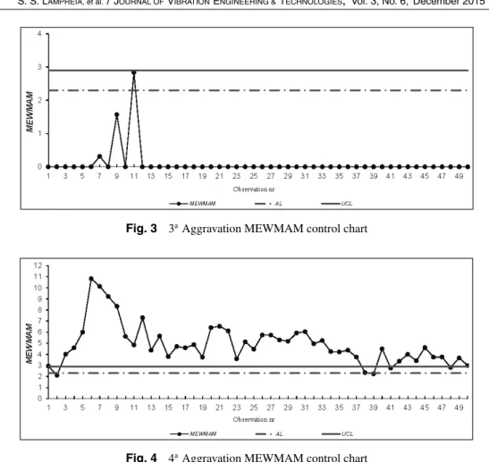
Fig. 3 3aAggravation MEWMAM control chart
Fig. 4 4aAggravation MEWMAM control chart
Havingp = 4, according Crowder (1989) abacus, the limits for MEWMAM control charts are presented in Table 1, so theK1 is the Alert Level (2,1) andK(2,7) the Upper Control Limit.
The vibrations are monitored since the first data value. To test the control chart sensitivity, 50 individual observations were read with the electric pump in normal operation; then, to accelerate the degradation, an anomaly and its aggravation through 4 stages was introduced.
Building the MEWMAM control chart to monitor the equipment, until the second aggravation no point is shown in the control charts.
For the third aggravation 3 points appear, all of them are under the UCL (Fig. 3).
The use of MEWMAM control chart shows a high level of sensitivity because after the third obser-vation almost all of the data are above the upper control limit, Fig. 4.
4.2 Data simulation – gas turbine
The equipment under study is a split-shaft Gas Turbine with a thermal efficiency of 37%, 19575 kW and a power velocity of 3600 rpm.
Fig. 5 Phase I –T2control chart
The LM2500 Gas Turbine has two parts, the Gas Generator (GG) and the Power Turbine (PT). The compressor, combustion chamber and the high pressure Turbine compose the GG.
Four sensors are considered in this study: the self and induced gas generator vibration sensors and the self and induced power turbine vibration sensors.
To illustrate the methodology application to propulsion equipment, based on collected real data from the gas turbine, 200 bootstrap samples were generated out of the observed data, using the resampling MATLAB functionbootstrap[10] to define the equipment parameters on the Phase I. On Phase II the mean and standard deviation were varied to simulate anomalies and to test the control chart sensitiveness to this kind of data.
For each measured point the vibration amplitude unit is expressed in mm, and it represents the vibration global value. Before the data simulation, the gas turbine was assumed to be working for 30 minutes.
The manufacturer characteristics define the vibration limits. For the gas generator at 4 mils there is an alert, and at 7 mils the gas turbine stops. For the power turbine at 7 mils there is a warning, and to 10 mils of vibration the turbine there is an emergency stop.
The generated data using the procedurebootstrapfrom MATLAB was independent and normal[10]. Thus in the study we start to define the equipment parameters by applying theT2control chart for the Phase I.
4.2.1 Phase I –TTT222control chart
In the application ofT2for simulated data the control limits are obtained from Table 1. See Fig. 5. All observations are under the upper control limit, thus control charts parameters can be estimated. The mean vector and the covariance inverse matrix are given by:
¯ X= ⎡ ⎢ ⎢ ⎢ ⎣
93,11 93,34 90,63 73,88
⎤ ⎥ ⎥ ⎥ ⎦ S= ⎡ ⎢ ⎢ ⎢ ⎣
0,27225 0,15876 0,08245 0,20297 0,15828 0,51654 0,07243 0,13266 0,08245 0,07243 0,25392 0,31507 0,20297 0,13266 0,31507 0,73457
⎤
⎥ ⎥ ⎥ ⎦
S−1= ⎡
⎢ ⎢ ⎢ ⎣
5,4 −1,343 0,385 −1,412
−1.3429 2,4 −0,3624 0,0979 0,3847 −0,3624 8,48 −3,678
−1,412 0,09792 −3,678 3,31
⎤
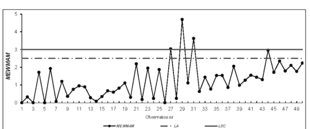
Fig. 6 Phase II – MEWMAM – 3rdanomaly aggravation
Fig. 7 Phase II – MEWMAM – 4thanomaly aggravation
4.2.2 Phase II – MEWMAM control chart
As for the electro-pump, the data were monitored since the first observation. The values were generated varying the mean and the standard deviation, consideringn=1, and 50 observations were generated for each situation of aggravation. The considered limits were:
TL= ⎡
⎢ ⎢ ⎢ ⎣
100,035 176,606 100,739 176,448
⎤
⎥ ⎥ ⎥ ⎦
In this data simulation for gas turbine,p =4, and the Crowder (1989) abacus for the MEWMAM control chart limits supplied an alert level ofK1=2.5, and an upper control limit ofK=3.
In Fig. 6, for the 3rdanomaly aggravation, three non-consecutive observations above the UCL can be noticed. Applying the rules, there is no need for a preventive intervention.
5
Conclusions
The Statistical Process Control was modified to account for the objective of equipment monitoring. To monitor equipment working condition, the limits should be defined by normative or by the manufacturer.
For the prototype, in Phase I, auto-correlation was detected in data. According to rules,T2control charts were applied using the residues from a fitted ARIMA model. On the Phase II, the MEWMA was applied to the expected values; high sensitivity was shown only after the 4thanomaly aggravation.
For the gas turbine, the application ofT2Mcontrol chart (T2modified control chart) is also possible for the Phase I, using simulated data. In Phase II, the gas turbine monitoring in working condition is possible using the MEWMAM control chart based on the calculated parameters.
Results from the prototype and from the gas turbine support the fact that equipment vibration monitoring is possible using the developed methodology for the Phase I and Phase II.
In spite of the results from Phase II for the referred equipment, it is considered that more tests, and maybe application to other equipment, should be carried out.
The application of a special multivariate control chart allows fast detection of eventual anomalies. The developed methodology will contribute to avoid unexpected equipment failures, increasing the operational reliability and the availability.
References
[1] Dias, J. M., Requeijo, J. G., Leal, R. P. and Pereira, Z. L., Optimizac¸˜ao do per´ıodo de substituic¸˜ao preventiva de componentes em func¸˜ao dos custos, (Optimization period component preventive replacement as a costs function),Manutenc¸˜ao, Nr 94/95, 3/4◦Trimester, APMI, 2007.
[2] Randall, R. B., Vibration-based condition monitoring – industrial, aerospace and automotive appli-cations, John Wiley & Sons, United Kingdom, 2011.
[3] Lampreia, S., Requeijo, J., Dias, J. and Vairinhos, V., T2 charts applied to mechanical equip-ment condition control, IEEE 16th,International Conference on Intelligent Engineering Systems 2012-INES2012, Caparica, 2012.
[4] Pereira, Z. L. and Requeijo, J., Qualidade: Planeamento e controlo estat´ıstico de processos, (Quality: Planning and Statistical Process Control), FCT/UNL, Pref´acio, Lisboa, 2012.
[5] Requeijo, J., Lampreia, S., Barbosa, P. and Dias, J., Controlo de condic¸˜ao de equipamentos mecˆanicos por an´alise de vibrac¸˜oes com dados auto correlacionados, (Control provided by mechanical vibration analysis with autocorrelated data), Riscos, Seguranc¸a e Fiabilidade, (Risks, Safety and Reliability), Salamandra, Lisboa, Vol. 1, pp. 483–497, 2012.
[6] Montgomery, D. C., Introduc¸˜ao ao controle estat´ıstico da qualidade, (Introduction to Quality Statistical Control), John Wiley & Sons Inc, USA, 2001.
[7] Box, E. P., Jenkins, G. M. and Reinsel, G. C., Time series analysis, forecasting and control (Third Edition), Prentice Hall, 1994.
[8] Zou, C. and Tsung, F., A multivariate sign EWMA control chart,Technometrics, Vol. 53, 84–97, 2011.
[9] Crowder, S., A simple method for studying run length distributions of exponentially weighted moving average,Technometrics, Vol. 29, pp. 155–162, 1989.