Annales
Geophysicae
Nonlinear (MARS) modeling of long-term variations of surface
UV-B radiation as revealed from the analysis of Belsk, Poland data
for the period 1976–2000
J. W. Krzy´scin
Institute of Geophysics, Polish Academy of Sciences, Warsaw, Poland
Received: 4 July 2002 – Revised: 4 February 2003 – Accepted: 13 February 2003
Abstract. A new, powerful statistical technique, multivari-ate adaptive regression splines (MARS), is applied to re-produce monthly fractional deviations of UV-B doses over Belsk, Poland, during the snowless (May–October) part of the year in the period 1976–2000. Two kinds of regressors were used: local ones (total ozone, percentage of sky cov-ered by low-, mid-, high-level clouds or total solar radiation over Belsk) and non-local ones, i.e. those describing the long-distance forcings on the surface UV-B due to changes in the global atmospheric circulation. Standard indices of the Quasi-Biennial, North Atlantic, El Ni˜no-Southern Oscil-lations, and the 11-year solar activity were used as non-local regressors. The results there indicate that the MARS pro-cedure is able to reproduce the observed year-to-year and decadal oscillations in the UV data. The MARS model yields better model-observation agreement than an ordinary least-squares fit based on the same set of regressors. It is found that MARS is capable of handling interactions between the lo-cal and non-lolo-cal regressors, suggesting a possible nonlinear nature of connections between variables characterizing the atmospheric transparency over Belsk and the long-distance forcings. MARS enables a reconstruction of the surface UV-B variations over any site based on the cloud and ozone data presently stored on web pages.
Key words. Atmospheric composition and structure
(aerosols and particles; biosphere-atmosphere interactions)
1 Introduction
Regression modeling is a widely used statistical technique to formulate a reasonable model of the relationship between a response variable and its predictors. Most research in time series modeling was carried out with linear models. How-ever, linear models may not adequately handle nonlinear time dependent systems. Radiative transfer through the atmo-sphere under cloudy conditions can serve as an example of Correspondence to:J. W. Krzy´scin ([email protected])
nonlinear interactions in the atmosphere. For example, due to multiple scattering of the solar radiation by clouds located on different levels (i.e. low, mid-, and high-level clouds), the measured solar irradiation at the ground level does not de-pend linearly on the cloud amount on each cloud level. It should be noted that various time scales have to be consid-ered to examine variations of the surface radiation, starting from scales of a few minutes related to the formation of in-dividual clouds and ending up on time scales of a few years (e.g. the North Atlantic Oscillations impact on cloudiness) and even decades (e.g. global warming impact on clouds structure). The equations describing the atmospheric system contain nonlinear terms (see, for example, term vi∂vk/∂xi
in the Navier-Stockes equations), leading to the necessity of testing a nonlinear approach in a statistical modeling of the atmosphere.
1888 J. W. Krzy´scin: Long-term variations of surface UV-B surface UV-B and examine how known long-term forcings
on the atmosphere dynamics (11-year solar cycle, Quasi-Biennial Oscillations – QBO, El Ni˜no-Southern Oscillations – ENSO, the North Atlantic Oscillations- NAO) affect the surface UV-B radiation.
Specifically, the research goal is to detect to what extent the departures of UV-B monthly means from the long-term (1976–2000) monthly means (normalized by the long-term means), i.e. the so-called fractional deviations obtained from the daily dose measurements carried out at Belsk (52◦N, 21◦E), are related to the changes in local (referring to a given site) forcing parameters and non-local (external) forcings due to variations of the global circulation pattern of the atmo-sphere. The time series of surface UV-B irradiance are rather short, usually not longer than 1 decade. As far as it is known to the author, one of the longer time series, which underwent the quality control procedure, comes from Belsk, Borkowski (2000). Thus, examinations of the Belsk’s time series may provide a basis for the surface UV reconstruction over any site that will take into account past total ozone data (from ground-based observations by the Dobson or Brewer spec-trophotometer, or satellite observations by the TOMS) and meteorological data (ground-based or satellite measurements of cloudiness, or surface total radiation by pyranometer mea-surements).
2 Data
In this section we define variables used in our regression models, i.e. a dependent variable (monthly fractional devia-tions of the erythemaly UV-B doses for Belsk), local regres-sors pertaining to the data collected at Belsk (total ozone, total solar radiation) or interpolated to this site (part of the sky covered by low-, mid- and high-level clouds that are de-rived from the National Centers for Environmental Predic-tion, (NCEP), U.S.A. reanalysis data), and non-local (exter-nal) regressors taken as indices of the global atmospheric circulation and other long-distance forcings (NAO, QBO, ENSO, and the 11-year solar cycle).
2.1 Dependent variable
The UV-B radiation measurements at Belsk have been car-ried out by means of the Robertson-Berger (RB) instrument in the period 1976–1992, Solar Light (SL) UV-Biometer 501A since 1991, and the Brewer spectrophotometer Mark II 64 since 1993. The RB meter and SL UV-Biometer are broad-band sensors for monitoring biologically active radia-tion. The instruments’ spectral characteristics were design to mimic the spectral sensitivity of Caucasian skin to sunburn (i.e. the erythema action spectrum, whose analytical form is given by the CIE action spectrum, McKinlay and Diffey, 1987). Their outputs were given in units of minimum ery-themal dose (MED) per hour. One MED is the dose of UV required to produce slight redness in an average fair-skinned person.
The daily sums of the instrument readings (daily doses) have been averaged for each month since January 1976 and used in our statistical analyses. Calibration of the Belsk RB instrument and a homogenization of the Belsk UV time se-ries were discussed by Krzy´scin (1996), Borkowski (1998), Borkowski (2000), and Krzy´scin (2000). The quality of the UV measurements by the Brewer spectrophotometer has been assured by comparisons each year with the traveling standard Brewer 17. The analyzed UV time series com-prises the homogenized RB time series for the period 1976– 1992, and that from 5-min scans by the SL UV-Biometer since January 1993. The estimated uncertainty (by the pro-ducer) of the daily dose by the SL UV Biometer is∼ ±5%. Slow time drift of sensitivity of our UV instruments needs to be checked. Our quality control/homogenization proce-dure takes into account the instruments’ behavior during the period of overlapped UV observations and radiative transfer model calculations of the expected RB readings for cloudless conditions.
The SL UV-Biometer data have been corrected by apply-ing the statistical relationship between the UV irradiances by the Brewer spectrophotometer and those by the UV-Biometer measured under clear-sky conditions. The reason why the SL UV-biometer data were used here instead of the Brewer data is the larger number of UV daily scans by the biome-ter (the Brewer spectrophotomebiome-ter also measures total ozone and SO2) and the continuous period of observations
through-out the year (every year there is a 2–3 week gap in the Brewer observations due to international intercomparisons).
2.2 Regressors
The total ozone observations have been conducted at Belsk since March 1963 by means of the Dobson spectrophotome-ter. All ozone observations have been reevaluated reading-by-reading using the Bass-Paur scale (Bass and Paur, 1985) recommended by the WMO and the calibration record of the instrument (Rajewska et al., 2000). The uncertainty of total O3measured by the Dobson instrument is estimated below
1% for the direct Sun observations and∼2–3% for the obser-vations using the UV irradiances coming from zenith under cloudy conditions.
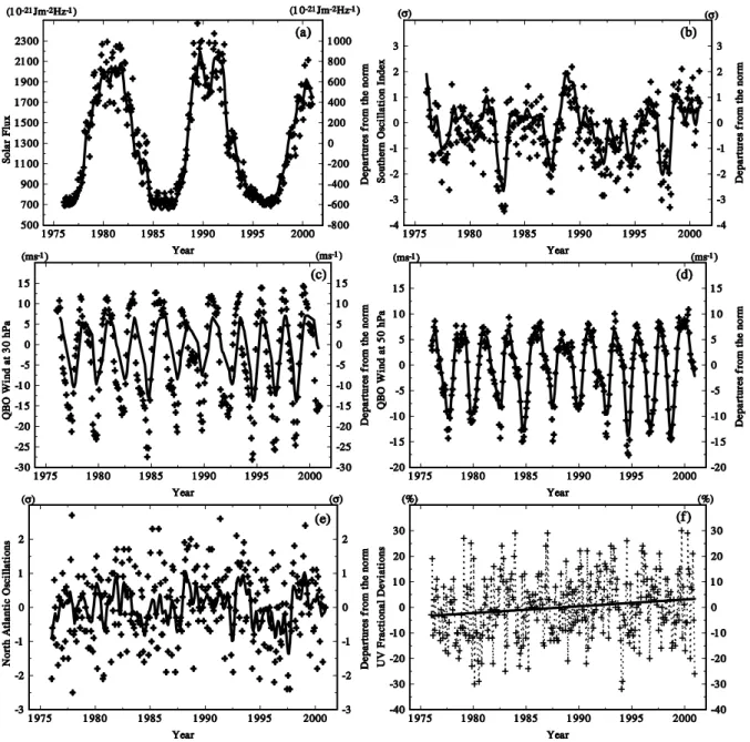
Fig. 1.The time series (1976–2000) of regressors explaining the surface UV-B variations;(a)the 11-year solar activity (10.7 cm solar flux at Penticton/Ottawa);(b)El Ni˜no-Southern Oscillations (normalized surface pressure difference between Tahiti – Darwin);(c)and(d) Quasi-Biennial Oscillations (zonal component of wind over the equatorial region) at 30 hPa and 50 hPa, respectively;(e)North Atlantic Oscillations (normalized amplitude of the leading mode of 700 hPa geopotential field disturbances over Northern Hemisphere). Fractional deviations of the monthly means of UV-B daily doses (erythemaly weighted) measured at Belsk for the period 1976–2000 – Fig. 1f. Solid curves in Figs. 1a–e represent the time series of regressors after removal of linear trend component and application a smoother (LOWESS) to resultant detrended time series. The straight line in Fig. 1f illustrates the linear trend in the data shown calculated by an ordinary least-squares fit.
measurements per month) than those for the daily measure-ments.
In so far, all discussed variables come from the measure-ments carried out at Belsk. It also seems interesting to an-alyze the cloud characteristics, i.e. amount of cloudiness by low-, mid-, and high-level clouds, from the combined ground-based/satellite observations. Here, the cloud sub-set of NCEP Reanalysis data, stored on the web page http: //wesley.wwb.noaa.gov/ncep data/, is considered. Gridded values of cloud cover by low-, mid-, and high-level clouds
interpolated to Belsk’s location are used as the local regres-sors. Further in our analyses, all the quantities mentioned in Sect. 2.1 and 2.2 are converted to fractional deviations, i.e. departures of actual monthly values from its monthly references (the 1976–2000 monthly means) in percent of the reference values.
1890 J. W. Krzy´scin: Long-term variations of surface UV-B standard indices are considered:
– Southern Oscillation Index (SOI) – the normalized sur-face pressure difference between Tahiti and Darwin, used as ENSO index,
– Zonal component of wind at 30 and 50 hPa level aver-aged over the region 5◦S–5◦N (wind data from NCEP Reanalysis) parameterizing the QBO effects on UV-B level,
– Normalized amplitude of the leading mode of 700 hPa geopotential field disturbances over Northern Hemi-sphere pertaining the NAO oscillations (presently avail-able on the web page http://www.cpc.ncep.noaa.gov/ data/teledoc/nao.html),
– 10.7 cm solar radio flux measured at Penticton/Ottawa, adjusted for the Sun-Earth distance, used to describe an external forcing on the atmosphere by the long-term so-lar activity.
Two kinds of regressors will be examined: rough monthly means (points in Figs. 1a–e) and smoothed monthly depar-tures (curves in Figs. 1a–e) that remain after subtracting the trend line (straight line fitted to the data by an ordinary least-squares regression) from the data and smoothing the resultant (detrended) time series. We use Locally Weighted Regres-sion – LOWESS to suppress month-to-month oscillations in the data. At each point in the data set a low-degree poly-nomial is fit to a subset of the data, with dependent variable values near the point whose smooth value is being estimated. The polynomial is fit using weighted least squares, giving more weight to points near the point whose response is be-ing estimated and less weight to points further away. The smooth value for the point is then obtained by evaluating the local polynomial using the dependent variable value for that data point (Cleveland and Devlin, 1988).
Figure 1f illustrates the variations of the monthly UV-B fractional deviations for the 1976–2000 period. The trend of ∼3–4% per decade (by an ordinary least-squares fit) is found over that period. Further in the analyses we will examine part of the UV data shown in Fig. 1f, i.e. the fractional deviations of UV monthly means for the snowless periods of the year (May through October) when the UV irradiance is especially high. The mean cumulative dose in that period constitutes about 80% of the total annual dose. Special attention has to be paid to the UV data collected in the snowless period of the year because of the natural high intensity of the UV-B radiation there.
3 Regression models
Two kinds of statistical models are examined here. First, one incorporates an advanced statistical technique able to capture both the linear and nonlinear impact of regressors on the de-pendant variable, Multivariate Adaptive Regression Splines (MARS), initially introduced by Friedman (1991). Second,
the model is a standard, stepwise regression selecting the best subset of the regressors (those significantly affecting the UV fractional deviations) from all local and non-local ones men-tioned in the previous section. MARS reveals a relationship between the dependent variable and independent ones (re-gressors). It has been applied in a wide range of disciplines (e.g. Lewis and Stevens, 1991; De Veaux et al., 1993a; Tal-iani et al., 1996; and Finizio and Palmieri, 1998). However, we decide to present below a short description of this method because it is a rather new tool of the time series analysis.
MARS starts from an assumption that all selected regres-sors affect the dependent variable in a complex way. There-fore, when MARS considers whether to keep a regressor in a model, it simultaneously searches for appropriate break points (known as knots). Models are constructed in a two-stage procedure. Stage I is a fast search that tests all database fields and potential break points, resulting in an overfitted model. Stage II refines the model by eliminating unneces-sary redundant regressors. The final model retains only the important variable (variables significantly affecting the out-come of the model). For an exhaustive description, refer-ence should be made to Friedman (1991). The great advan-tage of MARS is that it performs the selection of regressors, the interaction order between regressors, and the amount of smoothing, all automatically. This is accomplished via a pe-nalized residual sum of squares. The user can tune the degree of penalization, which depends on the number of regressors. On problems with a reasonably small number of predictors and where high order interactions do not dominate, MARS competes very favorably with nonlinear models, such as arti-ficial neural networks (De Veaux et al., 1993b). The authors suggested that MARS could be used instead of neural nets in a wide variety of applications, because MARS was always much faster and more interpretable than a neural net and was often more accurate as well.
MARS estimates of the UV monthly fractional deviations,
U V (t ), usingNregressorsxi(t ), when the assumed order of
the interactions between regressors is a two-way interaction (∼xixj), is as follows;
U V (t )=
N X
i=1
fa(xi(t ))+ N X
i,j,j >i
fb(xi(t ), xj(t ))+Noise(t)
Noise(t)=δNoise(t−1)+Random(t), (1) where the model residuals, N oise(t ), are modeled as first order autoregressive process, and
fa(xi(t ))= Li X
l=1
(αil,1(xi(t )−xoil)++αil,2(xi(t )−xoil)−)(2)
fb(xi(t ), xj(t ))=
Lj
X
m=1
Li
X
l=1
(βij,lm,1(xi(t )−xoil)+(xj(t )−xoj m)++
βij,lm,3(xi(t )−xoil)−(xj(t )−xoml)++
βij,lm,4(xi(t )−xoil)−(xj(t )−xoml)−). (3)
Functions(xi(t )−xo...)−and(xi(t )−xo...)+are linear right and left truncated splines, respectively. The minus (plus) sign after the parentheses indicates that this function equals
(xi(t )−xo...)forxi ≤ xo...(xi ≥ xo...), otherwise 0. In the
forward step, the MARS algorithm looks for partition points
xo...(the so-called knots,Lkdenotes the number of knots for
variablexk),α(...),β(...), are determined by straightforward
least-squares regression with fixed knots. In the backward step, MARS carried out a trimming procedure to remove terms of Eqs. (2) and (3), which do not remarkably contribute to the quality of the fit. In order to evaluate the quality of the model fit, MARS uses residual square errors penalized by a function depending onMI N– number of retained regression coefficients. The minimum of the following function,
GCV (MI N )= 1/S
S P
i=1
[U V (ti)−U Vmod,MI N(ti)]2
[1−C(MI N )/S]2 (4)
is used as a criterion (the so-called generalized cross valida-tion, GCV, criterion) to choose a final model. The numerator in GCV is the average residual squared error (S is the num-ber of data points andU Vmod,MI N(ti)are model fitted
val-ues) and the denominator is a penalty term that reflects model complexity. A model complexity penalty functionC(MI N )
increases inMI Nto prohibit selection of a model with many terms that improve only slightly the residual errors (for de-tails, see Friedman, 1991). In previous applications of the MARS technique in time series analyses, it was assumed that the residual term of the model had properties of random noise. Here the noise term of Eq. (1) is modeled as a first order autoregressive process to account for a part of the UV variations not explained by the regressors used. Both ver-sions (with and without the autoregression term) of model (1) were run and the better one was selected, i.e. that provid-ing the lower value of GCV.
The modeled time series of the fractional UV variations during the snowless part of the year for the period 1976–2000 by MARS is compared with those modeled by a standard stepwise regression, selecting the best set of regressors from all local and non-local ones. To be consistent with the two-way interactions assumed by MARS, our stepwise regression also includes these kinds of terms;
U V (t )= const+
N X
i=1
α∗ixi(t )+ N X
i,j,j≥i
βij∗xi(t )xj(t )+Noise,(5)
whereαi∗andβij∗ are regression constants to be determined by a standard least-squares procedure.
4 Results
To compare how various models reproduce original data we examine the percent of the variance of original data that is ex-plained by each model. Models defined by Eqs. (1) and (5)
may contain many terms, so it is possible that a little better fit to observed UV fractional deviations is due to a much larger number of the model’s terms used. Thus, to define a perfor-mance of each model we examine the adjusted total variance explained by the model, Adj.R2, that weighs the variance explained by model, R2, using the following formula, de-pending on the number k being the number of statistically significant terms of the model, i.e.
Adj.R2= (k−1)
(N−k)(1−R
2).
(6)
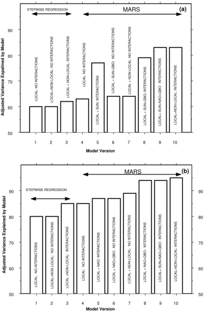
In Figs. 2a and b we showAdj.R2values by various MARS and stepwise regression models to find out how important are the interaction terms and non-local regressors in the statisti-cal modeling of UV variations. Figure 2a illustrates the re-sults obtained when part of the sky covered by low-, mid- and high-level clouds were among all regressors to be examined, whereas total solar radiation has been used instead of cloud cover for the results shown in Fig. 2b. In Sect. 4.1 we discuss the performance of the models using only local regressors and in Sect. 4.2 we show the results by models based on all available regressors and compare them with those shown in Sect. 4.1.
4.1 Effects of the local regressors
The maximum number of local regressors is 2 (measured to-tal ozone and toto-tal solar radiation values), or 4 (toto-tal ozone, percent of sky covered by low-, mid- and high-level clouds). It is worth mentioning that the latter case includes rather crude information of the monthly cloudiness (interpolated from the NCEP Reanalysis data) over Belsk. We would like to find what the gain is for model performance by use of the most proper (taking from the measured total irradiance at the observing site) proxy for the cloudiness impact on UV radi-ation.
It is seen (block no. 1 on Figs. 2a and b) that the stepwise regression using non-interacting local regressors (no terms
xi(t )xj(t )in Eq. 5) resolves∼60% and ∼80% of the total
variance. High-level clouds from NCEP Reanalysis appear to have a non-statistically significant impact on the UV frac-tional deviations. The UV response to the variations of total solar radiation or low-level clouds is the most pronounced among all analyzed regressors. Allowing for interactions be-tween local regressors (i.e. the stepwise regression using cloud data initially had 14 terms and that using total radi-ation had 5 terms) practically does not help to increase the
Adj.R2value, i.e. there is no need to account for the inter-actions between local regressors.
The MARS model using non-interactive local regressors (no functionfbin Eq. 1) yields slightly larger values of the
1892 J. W. Krzy´scin: Long-term variations of surface UV-B
1 2 3 4 5 6 7 8 9 10
Model Version
50 60 70 80 90
50 60 70 80 90
Adjusted Variance Explained by Model
LOCAL: NO INTERACTIONS
LOCAL+NON-LOCAL: INTERACTIONS
LOCAL+ SUN+NAO+QBO: INTERACTIONS
LOCAL + NAO+QBO: INTERACTIONS
LOCAL + NON-LOCAL: NO INTERACTIONS
LOCAL + NAO+QBO: NO INTERACTIONS
LOCAL + NAO: INTERACTIONS
LOCAL: NO INTERACTIONS
LOCAL +NON-LOCAL: INTERACTIONS
LOCAL+NON LOCAL: NO INTERACTIONS
STEPWISE REGRESSION
MARS (b) (a)
Model Version
1 2 3 4 5 6 7 8 9 10
50 60 70 80 90
Adjusted Variance Expalined by Model
LOCAL: NO INTERACTIONS
LOCAL+NON-LOCAL: INTERACTIONS
LOCAL+ SUN+NAO+QBO: INTERACTIONS
LOCAL + SUN+QBO: INTERACTIONS
LOCAL + NON-LOCAL: NO INTERACTIONS
LOCAL + SUN+QBO: NO INTERACTIONS
LOCAL + SUN: INTERACTIONS
LOCAL: NO INTERACTIONS
LOCAL + NON-LOCAL: INTERACTIONS
:LOCAL+NON-LOCAL: NO INTERACTIONS
STEPWISE REGRESSION MARS
Fig. 2.The adjusted variance,Adj.R2, explained by various statistical models including (or omitting) interactions be-tween the UV regressors and taking into account selected non-local regressors, shown in Figs. 1a–e, for the stepwise re-gression and MARS model. Figures 2a and b show the results for the cloud cover regressors and total solar radiance used as proxies for the cloud effects on UV, respectively.
much more complicated MARS than ordinary stepwise re-gression, if only local regressors are under consideration. 4.2 Effects of the non-local regressors
The correlation coefficients between the fractional UV devi-ations and the non-local regressors are rather small, i.e. the absolute values of the coefficients are less than 0.1. Thus, we cannot expect that a model containing linear terms propor-tional to the non-local regressors would help to explain a sig-nificant part of the UV variability. Stepwise regression, in-cluding the cloud-cover regressors among all possible regres-sors and excluding the interaction terms, contains initially 9 terms but finally, only local regressors remain. Allowing for interactions (thus initially the regression starts with 54 terms for the version using cloud cover regressors and 35 terms for the version with total solar radiance instead of cloud cover) helps to explain the additional 2% (for the cloud cover
re-gressors, see block no. 3 in Fig. 2a) and 5% (for the total solar radiation regressor, see block no. 3 in Fig. 2b).
MARS model, including the interactions between all local and non-local regressors, yields significantly largerAdj.R2
un-resolved by the best model. The standard deviation of the residuals is only 2.2%. The uncertainty of the UV daily dose observations (as given by the instrument producer) is esti-mated as±5% that can be transformed to an∼ ±1% uncer-tainty in the monthly mean doses. The remaining ∼1–2% of the monthly fractional deviations not resolved by the best model is probably related to the UV forcing variables not ac-counted for by the model regressors as, for example, specific aerosol characteristics (e.g. single scattering albedo, aerosol optical depth) and/or the vertical profile of the aerosol extinc-tion and ozone.
It is worth mentioning that the MARS model, taking into account the cloud cover regressors, which are rather crude proxies of the clouds effects on UV, provides slightly larger
Adj.R2 values than a simple regression model using total ozone and total solar radiance (known as an effective proxy for the cloud effects on UV) as the model regressors (com-pare block no. 10 in Fig. 2a and block no. 1 in Fig. 2b). We run several versions of the stepwise regression and MARS model with and without interaction terms, to find the most important set of non-local regressors (see block nos. 4–10 in Figs. 2a and b). We have found that SOI is not an effec-tive regressor as the versions with and without that predic-tor have almost the sameAdj.R2(see blocks no. 9 and no. 10 in Figs. 2a and b). If we decide to exclude two (three) non-local regressors by ranking their effects on UV radia-tion, MARS selects the NAO and QBO indices as the best pair of non-local regressors (NAO index as the single regres-sor), if total solar radiance is used as one of the regressors. When using the cloud-cover regressors among the local re-gressors MARS selects the 11-year solar cycle and QBO in-dex as the best pair of non-local regressors and the 11-year solar cycle as the best single non-local regressor. Both mod-els select different pairs of non-local regressors and single regressors having the largest impact on the UV radiance. It can be hypothesized that the 11-year solar cycle coupled with cloud-cover regressors provide an estimation of the cloud re-duction factor that is given straightforward by total solar ra-diation. Adding interaction terms improves significantly the model performance, especially when the cloud cover regres-sors are used (compare blocks no. 7 and 10 in Fig. 2a and those in Fig. 2b.).
5 Long-term variations of the UV radiation
The models selected in the previous section as the best in each category will be examined here to find out how they mimic the long-term pattern of the UV fractional deviations during the snowless part of the year in the period 1976–2000. We consider the following models:
– model A – selected by the stepwise regression with in-teraction terms including total ozone, the cloud-cover by mid- and low-level clouds as local regressors and indices of the atmospheric circulations (11-year solar cycle, QBO, and NAO) as non-local regressors
1894 J. W. Krzy´scin: Long-term variations of surface UV-B
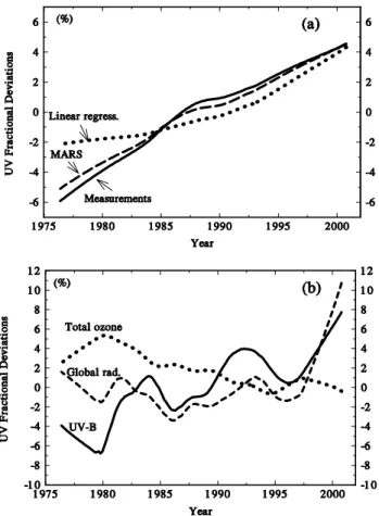
Fig. 4.The observed (solid curve) and modeled decadal variations of the UV fractional deviations for the snowless part of the year in the 1976–2000 period by stepwise regression (Model A – dot-ted curve) and MARS model (Model D – dashed curve) – Fig. 4a. The observed year-to-year variations in the UV fractional devia-tions (solid curve), total ozone (dotted curve), and total solar radia-tion (dashed line) – Fig. 4b. LOWESS smoother is used to extract decadal and year-to-year variations in the analyzed time series.
formance of this model is visualized by block no. 3 in Fig. 2a),
– model B – the same as model A but total solar radiation is used as a proxy for the cloud effects on the UV radi-ation instead of the cloud-cover by mid- and low-level clouds (see block no. 3 in Fig. 2b).
– model C – MARS model using the same regressors as model A, (see block no. 9 in Fig. 2a),
– model D – MARS model using the same regressors as model B, (see block no. 9 in Fig. 2b).
Figure 3 shows how the modeled long-term variations (with a time scale longer than a few years, see dotted curves in Fig. 3) resemble the observed ones (solid curves). It is seen that all models produce satisfactory results. Even a very simple model using crude parameterization of the cloud ef-fects on UV (model A) is able to reproduce the long-term variations. It provides a strong support for the quality of the cloud subset of NCEP Reanalysis data. The MARS model
(model C), based on the same set of regressors as model A, produces an even better model-observation agreement.
Figure 4a shows observed and modeled (model A and model D) decadal oscillations of the surface UV-B at Belsk for the snowless part of the year in the period 1976–2000. Here, the trend value will be inferred from a smoothed pattern of the UV oscillations derived by the LOWESS smoother that suppressed UV-B variations with time scales up to a decade. A steady increase of∼10% of surface UV-B at UV-Belsk is seen in that period. The rate of the UV in-crease was∼7% (linear trend of∼5.5% per decade) in the period 1975–1988, whereas only∼3% (linear trend∼2.5% per decade) in the period 1988–2000. Model D reproduces quite well the long-term oscillations of the surface UV-B. Model A is not able to reproduce the trend pattern over the first decade of observations and provides only a 6% increase in the surface UV-B for the whole period of observations. It should be noted that Fig. 4a shows the results of the best and the worst models discussed in this section (see theirAdj.R2
values shown in Figs. 2a and b). Model B, which contains the parameterization of the cloud effects on UV by means of the total solar radiations fluctuations, yields almost the same trend pattern as model D (compare modeled patterns of UV-B radiation in Figs. 3b and d).
A question immediately arises: what is the cause for the different trend values for the periods 1976–1988 and 1988– 2000? In Fig. 4b we present the smoothed (by LOWESS smoother) variations of surface UV-B superposed on total ozone and total solar radiation variations. It is seen that the larger UV increase in the former period was related to a high downward trend in total ozone, whereas a further positive trend of the UV-B radiation in the latter period was related to increasing atmospheric transparency (that was manifested as a positive tendency in total solar radiation there), because to-tal ozone remained rather stable over Belsk in that period. It is worth noting that the trend pattern shown in Fig. 4a was in-ferred, taking into account non-local regressors after removal of linear trend components and smoothing of the resultant trendless regressors. Thus, the calculated trend value of the surface UV-B radiation is a superposition of the total ozone and cloud/aerosol long-term effects on UV radiation.
6 Discussion
data were available, even if the total solar radiation was not measured there. It seems possible to reconstruct the past vari-ations of UV radiation for any site where the long-term time series of total ozone and the cloud reduction factor over the UV range (inferred from the total solar radiation data or the cloud amounts at different levels) are available. Our model is based on fractional deviations, so to estimate the necessary value of the UV norm (i.e. the mean value of UV radiation over the observation period) the clear sky value of the surface UV radiation by a radiative transfer model should be multi-plied by the mean value of cloud reduction factors over the UV range. For example, a formula derived by Matthijsen et al. (2000) can be used to relate a cloud reduction factor ob-tained from the attenuation of total solar radiation by clouds to that expected over the UV-B range.
The regression models examined here use indices of the atmospheric global oscillations as proxies of surface UV changes related to the long-distance forcings (teleconnec-tions). Thus, we assume that the atmospheric transparency over Belsk might have had specific properties resulting from the air mass advection controlled by the known long-term pe-riodical and unpepe-riodical oscillations in the atmosphere. For example, it looks possible that in periods when NAO is in its positive phase, the maritime aerosols will appear more frequently over Belsk, and the vertical profile of aerosols and ozone in the troposphere will also be disturbed there because of enhanced westerlies and above-average stormi-ness in those periods. Fluctuations of aerosol characteristics can be important sources of the UV variations, especially in snowless period. It was estimated that changes in aerosols optical depth have a comparable impact on the UV-B radia-tion as that induced by the total ozone changes. Day-to-day total ozone variations are rather small, about a few Dobsons, in that period (Krzy´scin and Puchalski, 1998, see their Ta-ble 1). The clouds appeared as the strongest modulator of the UV radiation over Belsk for all seasons.
Mayer et al. (1998) found that the transfer of UV-B radia-tion through the cloud layer could not be fully inferred from the observed cloud effects over different wavelength ranges (e.g. UV-A, whole spectral range 300–3000 nm, as in the case of total solar radiation). It should also be noted that total solar radiation is also sensitive to the amount of water vapour in the atmosphere, which has no direct effect on the surface UV. They found that the cloud reduction factor over the UV-B range is influenced mainly by three parameters: the optical depth of cloud, the amount of ozone within the clouds (combination of the ozone vertical profile and the position of cloud), and the absorption optical depth of aerosols. These three parameters were coupled nonlinearly in their effects on UV. So if we suppose that the cloud/aerosol properties are to some extent modulated by the long-term forcings, it will be possible to find the teleconnection effects on the surface UV-B radiation. More research studies are evidently needed to clarify this problem.
A comparison with previous studies dealing with the esti-mation of the surface UV radiation by regression models is not straightforward because of differences in the location of
the site where the UV observations were carried out, the UV variable to be estimated (absolute value, fractional deviation, non-weighted or weighted UV radiation), the data averaging procedure, and the length of the data period. It seems that the simplest way to compare the model behavior is to examine the value of the variance explained by a model. For exam-ple, the model by Matthijsen et al. (2000) resolved as much as 85% of the variance of the monthly means that were cal-culated by averaging daily doses of the erythemaly weighted irradiance for the period May–June–July of 1990, 1991, and 1992.
7 Conclusions
MARS is a rather new technique of the time series analysis that uses regression splines modeling and a recursive strat-egy to reproduce behaviour of a dependent variable using a limited number of regressors. Although MARS is a compu-tationally intensive regression methodology, it can produce models for high-dimensional data containing multiple par-titions and interactions between regressors. Here, MARS is used to reproduce the UV-B variations in the snowless part of the year for the period 1976–2000. It appears that MARS is capable of mimicing the behaviour of the observed data, es-pecially over longer time scales (see Fig. 3d for year-to-year variations and Fig. 4a for the decadal oscillations). It should be noted that MARS possibility provides the ability to model surface UV-B radiations over any site, if the total ozone data and estimates of the cloud reduction factor are both avail-able. The transparency of the atmosphere over the UV-B range due to changes in aerosols/cloud characteristics can be parameterized by MARS using the low-, mid-level cloud amounts (taken from NCEP Reanalysis data) or the total ra-diation data, and the indices of the atmospheric global cir-culation (QBO and NAO indices), and other external forcing (long-term solar activity described by the 10.7 cm solar flux). It should be noted that MARS is capable of handling interac-tions between the regressors, suggesting a possible nonlinear nature of connections between local variables, characterizing the atmospheric transparency over Belsk and long-distance teleconnections patterns. In conclusion, the use of the MARS technique appears to be effective in describing the nonlinear effects in the UV-B time series. Connections between atmo-spheric phenomena far apart in time and space, which could be hardly detected by other means, are also singled out and look very promising for further studies of coupling between the atmospheric global circulation and surface radiation.
Acknowledgements. The study has been supported by the
Commis-sion of the European Communities through EDUCE project con-tract no. EVK2-CT-1999-00028 and the Polish Committee for Sci-entific research under the grant no. 6 P04 D05717.
1896 J. W. Krzy´scin: Long-term variations of surface UV-B
References
Bass, A. M. and Paur, R. J.: The ultraviolet cross-sections of ozone: I. The measurements, in: Atmospheric ozone (Ed.) Zerefos, C. S. and Ghazi, A., Reidel, Dordrecht, Boston, Lancaster, pp. 606– 610, 1985.
Bodeker, G. E. and McKenzie, R. L.: An algorithm for inferring surface UV irradiance including cloud effects, J. Appl. Meteo-rol., 35, 1860–1877, 1996.
Bordewijk, J. A., Slaper, H., Reinen, H. A. M., and Schlamann, E.: Total solar radiation and the influence of clouds and aerosol on the biologically effective UV, Geophys. Res. Lett., 22, 2151– 2154, 1995.
Borkowski, J. L.: Revaluation of the time series of solar UV-B ra-diation data, Publs. Inst. Geophys. Pol. Acad. Sci. D-48(291), 81–89, 1998.
Borkowski, J. L.: Homogenization of the Belsk UV-B series (1976– 1997) and trend analysis, J. Geophys. Res., 105, 4873–4878, 2000.
Cleveland, W. S. and Devlin, S. J.: Locally Weighted Regression: An Approach to Regression Analysis by Local Fitting, J. Am. Stat. Assoc., 83, 596–610, 1988.
De Veaux, R., Gordon, A., and Comiso, J.: Modeling of topo-graphic effects on Antrarctic sea-ice using multivariate adaptive regression splines, J. Geophys. Res. Ocean, 98, 20 307–20 319, 1993a.
De Veaux, R., Psichogios, D., and Ungar, L. H.: A comparison of two nonparametric estimation schemes: MARS and Neural Networks, Computers in Chemical Engineering, 17, 819–837, 1993b.
Finizio, M. and Palmieri, S.: Non-linear modeling of monthly mean vorticity time changes; an application to the western Mediter-ranean, Ann. Geophysicae, 16, 116–124, 1998.
Friedman, J. H.: Multivariate adaptive regression splines, The An-nals of Statistics, 19, 1–50, 1991.
Ito, T., Sakoda, Y., Uekubo, T., Naganuma, H., Fukoda, M., and Hayashi, M.: Scientific application of UV-B observations from JMA network, Paper presented at 13th UOEH International Sym-posium and the Second Pan Pacific Cooperative SymSym-posium On Impact of Increased UV-B Exposure on Human Health and Ecosystem, Univ. of Occup. and Environ. Health, Kitakyushu, Japan, 1993.
Josefsson, W. and Landelius, T.: Effects of clouds on UV irradi-ance: As estimated from cloud amount, cxloud type,
precipi-tation, global radiation and sunshine duration, J. Geophys. Res., 105, 4927–4935, 2000.
Krzy´scin, J. W.: UV controlling factors and trends derived from ground-based measurements at Belsk, Poland, 1976-1994, J. Geophys. Res., 101, 16 797–16 805, 1996.
Krzy´scin, J. W. and Puchalski, S.: Aerosol impact on the surface UV radiation from ground-based measurements taken at Belsk, Poland, 1980–1996, J. Geophys. Res., 103, 16 175–16 181, 1998. Krzy´scin, J. W.: Total ozone influence on the surface UV-B radia-tion in the late spring summer 1963–1997: An analysis of multi-ple scales, J. Geophys. Res., 105, 4993–5000, 2000.
Lewis, P. A. and Stevens, J. G.: Nonlinear modeling of time series using multivariate adaptive regression splines (MARS), Journal of American Statistical Association, 86, 864–877, 1991. Matthijsen, J., Slaper, H., Reinen, H. A. J. M., and Velders, G. J.
M.: Reduction of solar UV by clouds: A comparison between satellite-derived cloud effects and ground-based radiation mea-surements, J. Geophys. Res., 105, 5069–5080, 2000.
Mayer, B., Kylling, A., Madronich, S., and Seckmeyer, G.: En-hanced absorption of UV radiation due to multiple scattering in clouds: Experimental evidence and theoretical explanation, J. Geophys. Res., 103, 32 241–32 254, 1998.
McArthur, L. J. B., Fioletov, V. E., Kerr, J. B., McElroy, C. T., and Wardle, D. I.: Derivation of UV-A irradiance from pyranometr measurements, J. Geophys. Res., 104, 30 139–30 151, 1999. McKinlay, A. and Diffey, B. L.: A reference action spectrum for
ul-traviolet induced erythema in human skin, in: Human Exposure to Ultraviolet Radiation: Risks and Regulation, pp. 83-87, Int. Congr. Ser., (Eds.) Passchier, W. F. and Bosnjakovich, B. F. M., Elsevier, New York, 1987.
Rajewska-Wiech, B., Deg´orska, M., and Krzy´scin, J. W.: An analy-sis of total ozone data from Belsk, obtained using the new (Bass-Paur) ozone absorption coefficients, Proceedings of the Quadren-nial Ozone Symposium, Sapporo, Japan 2000, (Eds.) Bojkov, R. and Shibasaki, K., 603–604, 2000.
Taliani, M., Palmieri, S., and Siani, A.: Visibility: an investigation based on a multivariate adaptive regression splines techniques, Meteorol. Appl., 3, 353–358, 1996.