Effects of the physical state of tropospheric ammonium-sulfate-nitrate particles on global aerosol direct radiative forcing

(1)

ACPD

3, 5399–5467, 2003

Effects of physical state of tropospheric

ammonium-sulfate-nitrate

particles

S. T. Martin et al.

Title Page Abstract Introduction Conclusions References

Tables Figures

◭ ◮

Back Close

Full Screen / Esc

Print Version

Interactive Discussion Atmos. Chem. Phys. Discuss., 3, 5399–5467, 2003

www.atmos-chem-phys.org/acpd/3/5399/ © European Geosciences Union 2003

Atmospheric Chemistry and Physics Discussions

E

_ff

ects of the physical state of

tropospheric ammonium-sulfate-nitrate

particles on global aerosol direct radiative

forcing

S. T. Martin1, H.-M. Hung1, R. J. Park1, 2, D. J. Jacob1, 2, R. J. D. Spurr3, K. V. Chance3, and M. Chin4, 5

1

Division of Engineering and Applied Sciences, Harvard University, USA 2

Department of Earth and Planetary Sciences, Harvard University, USA 3

Harvard-Smithsonian Center for Astrophysics, USA 4

School of Earth and Atmospheric Sciences, Georgia Institute of Technology, USA 5

Laboratory for Atmospheres, NASA Goddard Space Flight Center, USA

(2)

ACPD

3, 5399–5467, 2003

particles

S. T. Martin et al.

Tables Figures

◭ ◮

Back Close

Full Screen / Esc

Print Version

Interactive Discussion Abstract

The effect of aqueous versus crystalline sulfate-nitrate-ammonium tropospheric parti-cles on global aerosol direct radiative forcing is assessed. A global three-dimensional chemical transport model predicts sulfate, nitrate, and ammonium aerosol mass. An aerosol thermodynamics model is called twice, once for the upper side (US) and once 5

for lower side (LS) of the hysteresis loop of particle phase. On the LS, the sulfate mass budget is 40% solid ammonium sulfate, 12% letovicite, 11% ammonium bisulfate, and 37% aqueous. The LS nitrate mass budget is 26% solid ammonium nitrate, 7% aque-ous, and 67% gas-phase nitric acid release due to increased volatility upon crystalliza-tion. The LS ammonium budget is 45% solid ammonium sulfate, 10% letovicite, 6% 10

ammonium bisulfate, 4% ammonium nitrate, 7% ammonia release due to increased volatility, and 28% aqueous. LS aerosol water mass partitions as 22% effloresced to the gas-phase and 78% remaining as aerosol mass. The predicted US/LS global fields of aerosol mass are employed in a Mie scattering model to generate global US/LS aerosol optical properties, including scattering efficiency, single scattering albedo, and 15

asymmetry parameter. Global annual average LS optical depth and mass scattering e_fficiency are, respectively, 0.023 and 10.7 m2(g SO2₄−)−1, which compare to US val-ues of 0.030 and 13.9 m2(g SO2₄−)−1. Radiative transport is computed, first for a base case having no aerosol and then for the two global fields corresponding to the US and LS of the hysteresis loop. Regional, global, seasonal, and annual averages of top-of-20

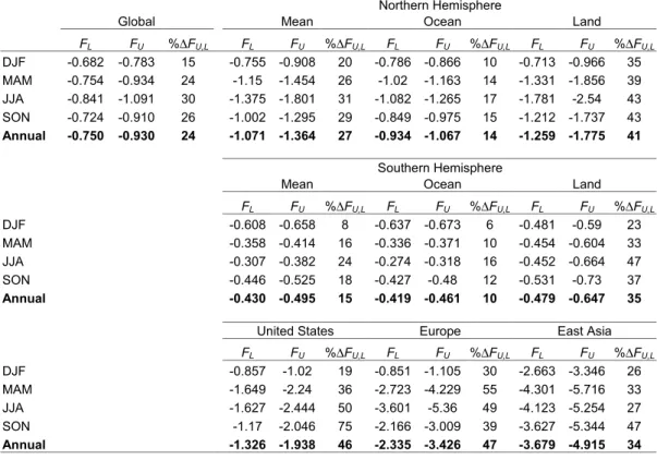
the-atmosphere aerosol radiative forcing on the LS and US (FL and FU, respectively, in W m−2) are calculated. Including both anthropogenic and natural emissions, we obtain global annual averages of F_L = −0.750, F_U = −0.930, and ∆F_U,L = 24% for full sky calculations without clouds andFL =−0.485,FU =−0.605, and∆FU,L =25% when clouds are included. Regionally,∆F_U,L =48% over the USA, 55% over Europe, 25

(3)

ACPD

3, 5399–5467, 2003

particles

S. T. Martin et al.

Tables Figures

◭ ◮

Back Close

Full Screen / Esc

Print Version

Interactive Discussion

G_L=−205 W (g SO2₄−)−1andG_U =−264 W (g SO2₄−)−1.

1. Introduction

Atmospheric aerosols significantly influence radiative transfer by scattering and ab-sorbing radiation (Houghton et al., 2001). The optical effects are strongly regulated by relative humidity (RH) because hygroscopic components absorb water, changing both 5

particle diameter and wavelength-dependent refractive indices (Martin, 2000).

Sulfate particles are the largest contributions to the global anthropogenic accumula-tion mode aerosol mass budget. Because they are nonabsorptive in the visible region of the electromagnetic spectrum, they provide the most significant anthropogenic cool-ing contribution to global direct radiative forccool-ing (Charlson et al., 1992; Seinfeld, 1996; 10

Haywood et al., 1997; Haywood and Boucher, 2000; Adams et al., 2001; Houghton et al., 2001; Jacobson, 2001a). Model predictions of the global distribution of anthro-pogenic and natural aerosol optical depth suggest that 40–60% of the annual average 550 nm aerosol optical depth over North America, Europe, and Asia and 28% over the globe is attributable to sulfate aerosol (Chin et al., 2002; Penner et al., 2002).

15

In the atmosphere, HNO3(g) and NH3(g) condense onto nonvolatile sulfate particles, yielding ionic particles of sulfate (SO2₄−), nitrate (NO−₃), ammonium (NH+₄), and pro-ton (H+). The SO2₄−−NO₃−−NH+₄−H+−H2O (SNA) particles are aqueous or crystalline (Martin, 2000). Their physical state affects the magnitude of aerosol direct radiative forcing, the partitioning of volatile species such as HNO3 between gas and particle 20

(Seinfeld and Pandis, 1998; Adams et al., 1999; Ansari and Pandis, 2000; Metzger et al., 2002), the rates of heterogeneous chemical reactions such as N2O5 hydrolysis (Mozurkewich and Calvert, 1988; Dentener and Crutzen, 1993; Hu and Abbatt, 1997; Kane et al., 2001), and the distributions and concentrations of O₃ via coupling of NO_y and Oxchemistry (Dentener and Crutzen, 1993; Jacob, 2000; Liao et al., 2003). 25

(4)

equi-ACPD

3, 5399–5467, 2003

particles

S. T. Martin et al.

Tables Figures

◭ ◮

Back Close

Full Screen / Esc

Print Version

Interactive Discussion librium and metastable branches of hygroscopic growth: physical state depends on the

RH history in an air parcel. Ammonium sulfate, for example, is crystalline up to 80% RH (cf. [1, 1] in Fig. 1c). At the deliquescence relative humidity (DRH) of 80% at 298 K, crystalline particles take up water and transform into aqueous droplets containing dis-solved NH+₄(aq) and SO2₄−(aq) ions. When RH decreases, aqueous ammonium sul-5

fate particles do not crystallize by homogeneous nucleation until the crystallization RH (CRH) of 35% is reached (efflorescence). Thus, between 35% and 80% RH, particles may be either aqueous or crystalline, depending on the RH history. This bifurcation is called the hysteresis loop (cf. Fig. 1c). Crystalline particles below the DRH follow the lower side (LS) (equilibrium branch) of the hysteresis loop while aqueous particles 10

above the CRH follow the upper side (US) (metastable branch). The major aim of our work is to compare the global aerosol direct radiative forcingF_LandF_U of SNA aerosol following the LS and US of the hysteresis loop.

1.1. Dependence of light scattering efficiency on aerosol phase

The reduction in intensityIof a directed beam along a path of thickness∆z(km) is: 15

I_z_+∆_z

Iz =

exp(−σ∆z)₌exp(−τ), (1)

where optical depthτ isσ∆z andσ (km−1) is the light scattering efficiency. Because light scattering by accumulation mode aerosol increases with the cross-section area of the particles, (mass)2/3is an approximate predictor of the dependence ofσ(km−1) on aerosol phase, overlooking variations in particle density, refractive index, and shape. 20

Figure 1c shows the predicted relative particle mass on the US and LS of the hysteresis loop for ionic compositions varying from acidic to neutralized.

The four hygroscopic growth curves in Fig. 1c are calculated (Clegg et al., 1998) for chemical compositions [0.4, 0.4], [0.6, 0.6], [0.8, 0.8], and [1, 1], where the coordinates [X, Y] refer to the SNA phase diagram shown at 298 K in Fig. 1a. The four corners 25

(5)

ACPD

3, 5399–5467, 2003

particles

S. T. Martin et al.

Tables Figures

◭ ◮

Back Close

Full Screen / Esc

Print Version

Interactive Discussion (Potukuchi and Wexler, 1995a,b). Coordinate X is the cation mole fraction arising

from NH+₄, with the balance coming from H+. It is also the degree of neutralization. Coordinate Y is the anion mole fraction arising from SO2₄−, with the balance coming from NO−₃. Coordinate Z is relative humidity and comes out of the page towards the reader.

5

There are seven possible solid phases that crystallize from SNA. Regions separated by heavy black lines (Figs. 1a, b) show the first solid that reaches saturation with falling RH, although solid formation occurs only on the LS of the hysteresis loop. The con-tour value of the dashed lines specifies the RH at which solid saturation occurs for an evaporating aqueous solution. The thin solid lines show the composition trajectory 10

of the residual aqueous phase after a solid has formed and assuming no exchange of NH3or HNO3with the gas-phase. In the atmosphere, exchange of H2O, NH3, and HNO3between gas- and particle-phases must be considered, so the liquid composition trajectories are somewhat different.

The LS behavior predicted by the phase diagram can be complex (Wexler and Clegg, 15

2002) (cf. Fig. 1c). For instance, an aqueous [0.8, 0.8] solution is predicted to form ammonium sulfate at 72% RH. As ammonium sulfate is removed from solution, the remaining aqueous phase becomes more acidic and more nitrified, as indicated by the trajectory of the solid line. At 65% RH, the residual solution is predicted to saturate with letovicite, and two solids begin precipitating. The solution increases its nitrate content 20

until 57% RH, at which point the ammonium sulfate and letovicite crystals and the remaining aqueous phase combine to form 2AN·AS, letovicite, and residual aqueous phase. At 54% RH, the last of the aqueous phase crystallizes, and the three crystals are letovicite, 2AN·AS, and 3AN·AS.

Acidic solutions, such as [0.4, 0.4], have a much simpler behavior because they 25

(6)

ACPD

3, 5399–5467, 2003

particles

S. T. Martin et al.

Tables Figures

◭ ◮

Back Close

Full Screen / Esc

Print Version

Interactive Discussion composition, a global chemical transport model (CTM) of this system must include

both aerosol acidity and nitrate.

The effect of [X, Y] on the percent change ofσ(%∆σ) at 500 nm for aerosol on the LS versus US of the hysteresis loop is shown in Fig. 2 for several RH values. For example, %∆σ [1, 1]dry =194% at 70% RH. The largest differences are obtained for 5

[X, Y] approaching the AS pole, regardless of RH. However, the range of compositions having non-zero values increases with lower RH. The explanation is found in Figs. 1a, c, which together show that solids are increasingly thermodynamically favored throughout [X, Y] space with decreasing RH and that the mass difference between the US and LS of the hysteresis loop increases with rising RH. For some compositions, however, %∆σ

10

is maximum at RH values below those at which a solid phase first forms. For example, %∆σ[0.8, 0.8] increases from 6% to 53% as RH falls from 70% to 60%. This behavior is understood by examining the complex crystallization pathway of [0.8, 0.8], which involves a progression through several solid phases (Fig. 1c).

Figures 1a, b, which are drawn for 298 and 274 K, respectively, further show that solid 15

formation and hence the hysteresis loop depend strongly on temperature. The stability regions of LET, 2AN·AS, and 3AN·AS expand at the expense of AS, AN, and AHS. There is a general uplifting of the RH for solid formation with decreasing temperature, as indicated by the contour values in Fig. 1b, which are approximately 5% greater than those in Fig. 1a. In the atmosphere, di_fferences between the US and LS of the 20

hysteresis loop are greater in cold regions such as the middle troposphere (MT) and upper troposphere (UT) year round and the boundary layer (BL) high latitude winter.

1.2. Previous treatments of aerosol phase in global models

Previous global modeling treatments of aerosol phase include: (a) prediction of phase but not direct radiative forcing and not including nitrate (Colberg et al., 2003), (b) cal-25

(7)

ACPD

3, 5399–5467, 2003

particles

S. T. Martin et al.

Tables Figures

◭ ◮

Back Close

Full Screen / Esc

Print Version

Interactive Discussion 2000; Jacobson, 2001a), (c) simulation of SNA aerosol and calculation of radiative

forcing but with the assumption that the aerosol follows the US of the hysteresis loop (van Dorland et al., 1997; Adams et al., 1999; Adams et al., 2001), and (d) simulation of SNA aerosol composition with calculation of the effect of US versus LS hysteresis loop on forcing (Metzger et al., 2002). A literature survey of approaches to treating 5

hysteresis is provided in Adams et al. (1999).

Previous studies of categoryb(fixed chemical composition) find∆F_U,L=15 to 20%. Representative results are given in Table 3 of Boucher and Anderson (1995) and Ta-ble 1 of Haywood et al. (1997). An improved approach is to predict SNA aerosol chem-ical composition (variable chemchem-ical composition) (van Dorland et al., 1997; Adams et 10

al., 1999; Adams et al., 2001; Metzger et al., 2002). Adams et al. (2001) calculate F_U but notF_L, instead assuming that the aerosol remains aqueous, even below DRH. Metzger et al. (2002) report ∆F_U,L = 5%. Unfortunately, their results seem anoma-lous. They have a normalized radiative forcing of−55 W (g SO2₄−)−1(inferred from their Figs. 5b and 6a, b), which is several times lower than the IPCC summary (Table 6.4, 15

Penner et al., 2001). Since Metzger et al. (2002) depart strongly from other reports, we restrict comparisons of our SNA results to those of Adams et al. (1999, 2001).

1.3. Description of our approach

The global aerosol direct radiative forcings (FLandFU) for aerosol following the limiting scenarios of LS versus US behavior on the hysteresis loop are calculated. (1) A global 20

three-dimensional CTM (GEOS-CHEM) predicts seasonal mass distributions of sulfate, nitrate, and ammonium aerosol on a global latitude, longitude, and altitude grid. Het-erogeneous chemical reactions and gas-phase partitioning assume the aerosol is on the US of the hysteresis loop. (2) To produce the LS mass field, the chemical content of each grid box is analyzed to assess the thermodynamic driving force for crystalliza-25

(8)

ACPD

3, 5399–5467, 2003

particles

S. T. Martin et al.

Tables Figures

◭ ◮

Back Close

Full Screen / Esc

Print Version

Interactive Discussion than on the US (Ansari and Pandis, 2000). (3) In five shortwave spectral bands

(Ta-ble 1), LS and US global fields of aerosol optical properties, including mass scattering efficiency,β(m2g−1), single scattering albedo (ω), and asymmetry parameter (g), are calculated with Mie scattering theory. (4) Radiative transport for each longitude-latitude column is computed using the LIDORT discrete ordinate model (Spurr, 2002), first for 5

a base case having no aerosol and then for the two global aerosol fields correspond-ing to the US and LS of the hysteresis loop. Regional, global, seasonal, and annual averages ofFLandFU are calculated in the absence and presence of clouds.

2. Aerosol mass concentrations and chemical composition

A global 3D model of atmospheric aerosols and chemistry (GEOS-CHEM v5.03) is 10

employed to predict aerosol sulfate, nitrate, and ammonium mass (Park et al., 2003). Important aspects include SO2, NOx, and NH3 emissions, gas-phase and aqueous-phase chemical transformations to form sulfate, nitrate, and ammonium aerosol, and wet and dry deposition to remove species from the atmosphere.

2.1. Global chemical transport model 15

The CTM employs assimilated meteorological observations for 1998 from the Goddard Earth Observing System (GEOS) of the NASA Global Modeling and Assimilation Office (GMAO). The model resolution is 4◦ latitude by 5◦ longitude with 30 pressure levels. Initial conditions are set by running the model for 12 months (1998). The model is then run a second time for 1998 to collect seasonal results of sulfate, nitrate, and ammonium 20

mass concentrations from January 1998 onwards.

(9)

ACPD

3, 5399–5467, 2003

particles

S. T. Martin et al.

Tables Figures

◭ ◮

Back Close

Full Screen / Esc

Print Version

Interactive Discussion lightning, soils, and wildfires for NO_x, and soils and wildfires for NH₃. Formation of

aerosol sulfate and nitrate by oxidation of SO2 and NOx takes place by gas-phase and heterogeneous oxidation processes coupled to the oxidant chemistry in the model (Park et al., 2003). Aerosol and gas losses by wet deposition include scavenging in convective updrafts/anvils and rainout/washout from large-scale precipitation (Liu et 5

al., 2001). Dry deposition follows a standard resistance-in-series scheme based on the work of Wesely (1989) and is implemented as described by Wang et al. (1998).

2.2. Sulfate, nitrate, and ammonium distributions

2.2.1. Tropospheric burdens

Our annual average tropospheric aerosol sulfate burden is 0.37 Tg S (0.72 mg S m−2, 10

1.11 Tg SO2₄−), which is less than the average value of 0.77 Tg S (with a standard deviation of 0.19 Tg S) of nine previous studies (see Table 5.5 of Penner et al., 2001). A detailed explanation of this difference is given in Park et al. (2003). Our annual average tropospheric nitrate and ammonium burdens are 0.20 Tg NO−₃ and 0.37 Tg NH+₄, which compare to 0.13 Tg and 0.39 Tg, respectively, in Adams et al. (1999) (base run in their 15

Table 9). Metzger et al. (2002) report an average burden of 0.12 Tg NO−₃ (inferred from their Fig. 5a).

2.2.2. Column loadings and boundary layer concentrations

Our seasonal and geographic distributions for BL SNA aerosol mass (Fig. 3) and col-umn burdens (Fig. 4) agree well in form, though smaller in magnitude, with those in 20

(10)

ACPD

3, 5399–5467, 2003

particles

S. T. Martin et al.

Tables Figures

◭ ◮

Back Close

Full Screen / Esc

Print Version

Interactive Discussion tions over southern Africa and western South America are due to mining and smelting

(Spiro et al., 1992).

Because most aerosol sulfate is in the BL (Fig. 3), geographic distributions of column burdens roughly approximate those of the BL (Fig. 4). In comparison, BL concentra-tions of nitrate and ammonium are less accurate predictors of column burdens. The 5

implication is that nitrate and ammonium are mixed to a greater extent throughout the tropospheric column than sulfate.

One reason for this difference is that sulfate is nonvolatile, whereas HNO3(g) and NH3(g) are partially volatile. One of several alternative conditions must be met for HNO₃(g) and NH₃(g) to condense. For example, under cold conditions HNO₃(g) con-10

denses to make acidic aerosols. This mechanism is active in the upper atmosphere and in polar regions, but it does not occur at lower latitudes and altitudes because the temperature is too high. HNO3(g) also condenses when NH3(g) is in excess supply to form NH₄NO₃, except for hot summer regions. Thus, aerosol ammonium and nitrate mass are both reduced by warm temperatures and limited by insufficient NH3(g) or 15

HNO3(g).

A second reason for greater vertical mixing of nitrate and ammonium is that the sources of NOx and NH3 are different from those of SO2. The precursor NOx emis-sions in the USA, Europe, and Asia are combustion by-products associated with trans-portation and power production. Therefore, some nitrate is roughly co-located with 20

sulfate. However, there are also additional emissions. Biomass burning leads to ni-trate in Africa, Russia, and South America. Lightning is a significant NOxsource above the BL. The major ammonia emissions occur in geographic regions having intensive agriculture and livestock industry. The oceans are also a diffuse but important source. Biomass burning is approximately 10% of the emissions, but it is nevertheless impor-25

tant due to its temporal and geographic coincidence with NO_x emissions, leading to a synergy in the formation of aerosol NH4NO3.

(11)

ACPD

3, 5399–5467, 2003

particles

S. T. Martin et al.

Tables Figures

◭ ◮

Back Close

Full Screen / Esc

Print Version

Interactive Discussion concentrations, though the reverse is not always true because high ammonium also

correlates with increased sulfate. USA, Europe, and east Asia have both strong NO_x and NH3 emissions, and aerosol formation is apparent. However, the aerosol load-ing over east Asia and India does not increase proportionally to the ten-fold increase in NH₃ emissions in these regions because HNO₃(g) concentrations, while large, are 5

less than NH3. These regions are thus HNO3(g) limited, whereas USA and Europe are usually NH3limited. The latitudes above 60◦N have elevated nitrate concentrations in the cold seasons, as do those below 60◦S in the opposite season.

2.3. Comparisons of model predictions to observations

Observations of sulfate, nitrate, and ammonium concentrations worldwide are given in 10

Table 7 of Adams et al. (1999). Other important networks are the Clean Air Status and Trends Network (CASTNET) in the United States (EPA, 1999) and the Co-operative Programme for Monitoring and Evaluation of the Long-Range Transmission of Air Pol-lutants in Europe (EMEP) (Hjellbrekke, 2000). Quantitative evaluations of predicted sulfate, nitrate, and ammonium concentrations using observations at CASTNET and 15

EMEP sites are presented in Park et al. (2003). Therein, the model predictions gen-erally reproduce the annual and monthly mean concentrations to within a factor of two and capture the geographic distribution well in those regions.

In contrast to the traditional scatter plots of predicted versus observed loadings (Chin et al., 1996, 2000; Koch et al., 1999; Barth et al., 2000; Park et al., 2003), the relative 20

ratio among SNA species is the key element of our work. Phase predictions depend intensively onX andY rather than extensively on sulfate, nitrate, and ammonium con-centrations (Figs. 1a, b). We thus compare [X, Y]predicted to [X, Y]observedin Fig. 5. Be-cause the measurements are limited to sulfate, nitrate, and ammonium, we assume the proton concentration is given by charge balance, allowing us to calculate [X, Y]observed. 25

(12)

ACPD

3, 5399–5467, 2003

particles

S. T. Martin et al.

Tables Figures

◭ ◮

Back Close

Full Screen / Esc

Print Version

Interactive Discussion composition in the AN direction, viz. towards the [1, −1] pole in Fig. 5b. There is

also a bias towards AS for the global predictions for both our results and those of Adams et al. (1999). For both global and European predictions, the bias is explained by overprediction of the ammonium fraction. This result may indicate our ammonia emissions are too strong in some geographical regions and in some seasons (Park et 5

al., 2003).

2.4. Predicted ammonium and sulfate fractions (X andY)

2.4.1. Clustering of [X, Y] compositions

The [X, Y] predictions are shown in Fig. 6 for each model grid box in the BL, MT, UT, and the entire troposphere. The locus of points for the entire troposphere overlaps 10

strongly with compositions having %∆σ > 0 (Fig. 2). The implication is that phase transitions strongly influence the optical properties of tropospheric particles. In the BL, where most aerosol mass resides, aerosol chemical compositions cluster towards the AS pole [1, 1]. The consequence is an increased impact for phase transitions on the optical properties of BL aerosol (cf. Figs. 2 and 6). Employing areal longitude-latitude 15

averaging (without weighting for aerosol mass), the characteristic average composition in the BL is<X, Y >=[0.80, 0.93].

In the MT, aerosol is more acidic. Specifically,<X, Y>=[0.54, 0.94] in the MT and

∆ <X, Y > = [−0.26, +0.01] as compared to the BL. Increased acidification results because there are sulfur emissions from volcanoes and aircraft into the MT, while am-20

monia emissions are absent. Furthermore, nitrate is maintained by in situ sources such as lightning, and some of this nitrate condenses in cold regions. The consequence is a translation of the group of composition points in the direction of increased nitrate (Fig. 6). Further acidification occurs in northern hemisphere winter, partially because the shallower mixing depth in the cold season leads to inefficient vertical mixing of 25

(13)

ACPD

3, 5399–5467, 2003

particles

S. T. Martin et al.

Tables Figures

◭ ◮

Back Close

Full Screen / Esc

Print Version

Interactive Discussion Compositions in the UT are largely near the AN pole, especially in June through

November. The annual average<X, Y > is [0.69, 0.70]. The perturbations compared to the BL and MT are [−0.11,−0.23] and [+0.15,−0.24], respectively. The increase in nitrate is explained by condensation of nitric acid at cold upper tropospheric tempera-tures.

5

2.4.2. Global maps of [X, Y] compositions

Geographic prediction of [X, Y] (Fig. 7) is necessary to model the distribution of aerosol phase. Neutralized aerosol, which is more susceptible to crystallization than acidified aerosol, occurs throughout large regions of the BL. Acidified aerosol is common in regions overlying the oceanic gyres, which are isolated from anthropogenic NH3. In 10

Antarctica NH₄HSO₄ aerosol is prevalent, except during the cold austral winter when the aerosol is enriched in ammonium nitrate. In the northern hemisphere, there is much greater acidification in winter than in other seasons. The seasonal dependence arises because sulfate and nitrate precursor emissions vary weakly with time, having a maximum of sulfur emission in winter. In contrast, important ammonia sources have 15

a strong positive temperature dependence and are thus maximum in summer. The imbalance of acidic and alkaline precursor emissions results in more acidified particles in winter.

2.4.3. Comparison to previous studies

Our predictions of SNA aerosol composition (Fig. 6) can be compared to those of 20

Adams et al. (1999) (Plates 4b, c; annual average) and Metzger et al. (2002) (Fig. 3a; January and July 1997, surface layer). Adams et al. (1999) define the degree of neu-tralization (DON), which equalsX, and the nitrate-to-sulfate mole ratio (NTS), which is calculable from the relationY =1/(NTS+1). Metzger et al. (2002) provide global dis-tributions of nitrate fraction (NF), which equals 1−Y. To compare our results to those 25

(14)

ACPD

3, 5399–5467, 2003

particles

S. T. Martin et al.

Tables Figures

◭ ◮

Back Close

Full Screen / Esc

Print Version

Interactive Discussion NF plots (not shown). Our NF global plots agree in all qualitative features with those

of Metzger et al. (2002), except that we predict NF approaching unity over Antarctica in the austral winter. The nitrate fraction of Metzger et al. (2002) is also consistently slightly higher than our own global predictions.

Compared to the DON global plots of Adams et al. (1999), we obtain similar gen-5

eral geographic patterns in the lows and highs for the BL, though our results have a consistent offset towards greater neutralization. We obtain ∆X = +0.17 in the BL,

+0.16 in the MT, and +0.30 in the UT. These changes are relative to base values of X =0.63, 0.38 and 0.39. Our predictions for a significantly more neutralized aerosol are explained by a combination of factors. First, because we use lower sulfur emissions 10

(1998 versus 1990) but similar ammonia emissions, a more neutralized aerosol is an-ticipated. Second, nitric acid monthly average fields employed by Adams et al. (1999) are acknowledged by those authors as too high and thusX is systemically low. Third, because of finer model vertical resolution in our study (20 versus 7 layers), vertical mo-tion such as moist convecmo-tion is represented more accurately and increased vertical 15

transport results. As a consequence, ammonia gas is transported to the UT, and a more neutralized aerosol results.

These model differences affect the sulfate fraction to a lesser extent. We find∆Y = +0.01 in the BL,+0.01 in the MT, and−0.10 in the UT. These changes are relative to base values ofY = 0.92, 0.93 and 0.80 in Adams et al. (1999). There is thus good 20

agreement in the predicted annual average sulfate fraction. Our NTS global plots in the BL are consistent with the high values predicted by Adams et al. (1999) over central North America, Europe, and East Asia.

3. Aerosol physical state

The ISORROPIA thermodynamic model (Nenes et al., 1998) is called for a prediction 25

(15)

ACPD

3, 5399–5467, 2003

particles

S. T. Martin et al.

Tables Figures

◭ ◮

Back Close

Full Screen / Esc

Print Version

Interactive Discussion The geographic distribution of the predicted solids formed is shown in Fig. 8 for the BL,

MT, and UT. Definitions for the results shown in Fig. 8 are as follows:

%AS=100×n L AS

nU_S , %LET=100× 2nL_LET

nU_S , %AHS=100× nL_AHS

nU_S ,

%AN₌100×n L AN

nU_N ,%H2O=100× nL_H

2O

nU_H

2O

, (2)

wherenis moles. Subscripts are ammonium sulfate (AS), letovicite (LET), ammonium 5

bisulfate (AHS), ammonium nitrate (AN), particle water (H₂O), aqueous sulfate (S), and aqueous nitrate (N). SuperscriptsU and L indicate US and LS of the hysteresis loop. (ISORROPIA’s database contains only 4 of 7 SNA solids and thus differs from the AIM model (Clegg et al., 1998), employed by us to prepare Figs. 1 and 2. An intercomparison of thermodynamic models is provided by Zhang et al., 2000.)

10

When %H2O=100%, US and LS aerosol water is identical: aqueous particles are not metastable and no solids form. When %H₂O=0%, particles on the LS crystallize entirely and no residual aqueous fraction remains. When 0<%H2O<100%, particles partially crystallize and a residual aqueous layer remains. Sulfate partitioning into solid phases is given by %AS, %LET, and %AHS. Their sum is 100% when no particle 15

water remains (%H2O=0%). The fraction of US aqueous nitrate crystallizing on the LS into ammonium nitrate is %AN, whereas another fraction volatilizes as NH3(g) and HNO₃(g). When no particle water remains, %AN is generally less than 100% due to volatilization.

For the complete atmospheric burden (Sect. 2.2.1), the global annual average sulfate 20

(16)

ACPD

3, 5399–5467, 2003

particles

S. T. Martin et al.

Tables Figures

◭ ◮

Back Close

Full Screen / Esc

Print Version

Interactive Discussion AS, 10% LET, 6% AHS, 4% AN, 7% ammonia release due to increased volatility, and

28% aqueous. LS aerosol water mass partitions as 22% effloresced to the gas-phase and 78% remaining as aerosol mass. (The US aerosol water burden is 1.12 Tg.)

3.1. Geographic, seasonal, and altitude dependencies of solid formation

Geographic regions having %H₂O<100% show where solid formation is predicted on 5

the LS of the hysteresis loop (Fig. 8). Explaining why solids form in some locations but not in others requires simultaneous consideration of [X, Y], RH, and temperature T (Figs. 1a, b). Increased neutralization, drying, and cooling are factors favoring crys-tallization, each of which being a necessary if not sufficient condition.

3.1.1. Boundary layer 10

The expectation value for the global annual average LS water content in the BL is <%H₂O>=71% of the US value. The expectation value is calculated with areal longitude-latitude weighting (without weighting for the aerosol mass loading in each grid box). Compared to the oceans, the continents favor water loss and hence crys-tallization (Fig. 8a). Because neutralization is observed over wide regions of both the 15

continents and the oceans (Fig. 7), neutralization alone is not a sufficient explanation of preferential crystallization over the continents. Rather, solid formation over the con-tinents arises from lower RH, as compared to over the ocean. Figure 8a further shows crystallization in austral winter over Antarctica. Solid formation is attributed there both to the neutralization (Fig. 7) and cold temperatures.

20

When solids do form in the BL, AS is the principal form (Fig. 8a), as expected from the neutralized US aqueous aerosol (Fig. 7). Specifically, the expectation values of global annual average BL sulfate aerosol mass with areal weighting are 28% solid AS, 4% LET, 1% AHS, and 67% aqueous. By comparison, when the aerosol mass loading of each grid box is included in the average, the BL partitioning is 43% solid AS, 7% LET, 25

(17)

ACPD

3, 5399–5467, 2003

particles

S. T. Martin et al.

Tables Figures

◭ ◮

Back Close

Full Screen / Esc

Print Version

Interactive Discussion aerosol is more acidic in these regions. Letovicite is common in equatorial Africa.

Particles composed of all three sulfate solids are predicted in SON in the Antarctic. Solid AN is predicted for cold regions, including the poles and the northern winter hemisphere. In other regions such as warm equatorial Africa, for dry aerosol, AN en-tirely evaporates. This conclusion is reached by noting geographic regions having both 5

%H2O=0 and %AN=0 in Fig. 8a while simultaneously having significant US aerosol nitrate shown in Fig. 3. When weighted by aerosol mass loading of each grid box, annual average BL nitrate partitions as 15% AN, 72% volatilized, and 13% aqueous. A seasonal dependence is predicted for %AN. In JJA, %AN is close to zero everywhere outside of Antarctica, whereas in DJF, %AN> 0 in most of North America and Asia. 10

Solid AN is significant in Europe in MAM and SON.

3.1.2. Middle troposphere

Compared to the BL, the geographic coverage of predicted crystallization increases in the MT (Fig. 8b). <%H2O>drops from 71% in the BL to 49% in the MT. Cooling at higher altitude is the principal driver in the overall increase in crystallization (cf. Figs. 1a, 15

b), which leads to a further significant difference in the role of neutralization as a mod-ulator of the patterns of crystallization in the BL and MT. In the BL, because most of the aerosol is neutralized (Fig. 7) and thus of appropriate chemical composition to crystallize, the main modulator is RH. Above the BL, due to lowT and RH, many air parcels provide favorable conditions for crystallization; however, the aerosol acidity has 20

greater variability in the MT and thus neutralized aerosol chemical composition modu-lates crystallization (cf. Figs. 7 and 8b).

Predicted phase partitioning in the MT is shown in Fig. 8b. All three sulfate solids occur in significant amounts, their relative ratios depending upon season and location. The global annual average areal-weighted partitioning is 21% solid AS, 12% LET, 31% 25

(18)

ACPD

3, 5399–5467, 2003

particles

S. T. Martin et al.

Tables Figures

◭ ◮

Back Close

Full Screen / Esc

Print Version

Interactive Discussion predominates, residual particulate aqueous phase remains.

Ammonium nitrate has global coverage in the MT only in JJA. The causative agent is an increase in neutralization and nitrate content in this season (Fig. 7). Ammonium nitrate is also significant near India due to strong emissions and uplifting. AN is not predicted in the BL over India in JJA (Fig. 8a), yet it is present in the MT (Fig. 8b). 5

Figure 7 shows little change in extent of neutralization. The explanation is the drop in temperature with altitude. When weighted by aerosol mass loading of each grid box, annual average MT nitrate partitions as 17% AN, 82% AN volatilized, and 1% aqueous.

3.1.3. Upper troposphere

Predicted phase partitioning in the UT is shown in Fig. 8c. Unlike the MT and in stark 10

contrast to the BL, complete crystallization prevails in most locations. The global annual average<%H2O>is 12%. The driver is cold temperature. An exception is a decrease in crystallization in MAM in the southern hemisphere; this season and location are more acidified than all others (Fig. 7).

The global annual average areal-weighted partitioning is 45% solid AS, 16% LET, 15

30% AHS, and 9% aqueous. However, partitioning in the period June through Novem-ber is distinct from that of DecemNovem-ber through May. In the Jun–Nov period, AS and AN dominate the northern hemisphere while AHS is the prevalent phase in the south-ern hemisphere. In the Dec–May period, LET and AHS are dominant, except for the equatorial region where AS is found.

20

Throughout the year, AN coincides closely with AS. The explanation is in the precur-sor aqueous chemical composition: significant nitrate content is associated with neu-tralization and hence ammonium sulfate (Fig. 7). The same is also true of the BL and MT, and inspection of Figs. 8a, b shows AS and AN solids occur together. However, at warmer temperatures in the LT, AN volatilizes on the LS of the hysteresis loop and 25

(19)

ACPD

3, 5399–5467, 2003

particles

S. T. Martin et al.

Tables Figures

◭ ◮

Back Close

Full Screen / Esc

Print Version

Interactive Discussion 3.1.4. Comparison to previous studies

Employing fields of ammonium-to-sulfate ratios from Adams et al. (1999), Colberg et al. (2003) predict AS, LET, and AHS global distributions in the MT in July (Figs. 6 and 7 in Colberg et al., 2003). In Colberg et al. (2003), the aerosol is restricted to aqueous SO2₄−−NH+4−H+−H2O, compared to our work including NO−3. Thus Colberg 5

et al. (2003) neither predict AN formation nor include the effect of nitrate on sulfate solid formation; their study lies on the [X, 1] axis of Figs. 1a, b. These differences notwithstanding, the results of Colberg et al. (2003) agree with our predicted %H2O (JJA, Fig. 8b), showing that solid formation is prevalent in the northern hemisphere, while aqueous aerosol is found in the equatorial region outside of Africa.

10

Figures 6 and 7 of Colberg et al. (2003) assume the aerosol follows the US of the hysteresis loop. Apart from these two figures, the bulk of the Colberg et al. (2003) pa-per comprises a trajectory analysis to account for the hysteresis loop, and their results then lie partway between our limiting cases of US versus LS hysteresis behavior. We nevertheless compare Fig. 12 of Colberg et al. (2003) to our JJA Fig. 8b for predictions 15

of %AS, %LET, and %AHS. Predictions agree well for AHS regions dominant in a band through the southern hemisphere. Letovicite is also predicted for the northern hemi-sphere. However, we predict extensive regions of AS, which Colberg et al. (2003) do not. As discussed earlier, a reasonable explanation is that we predict a more neutral-ized tropospheric aerosol than Adams et al. (1999), upon which Colberg et al. (2003) 20

base their results.

3.2. Chemical composition of residual aqueous layers

The aqueous chemical compositions of particles following the LS of the hysteresis loop (Fig. 9) are described by three cases. (1) White regions, indicating complete crystal-lization and no residual aqueous composition, have %H2O=0 (Fig. 8). (There is water 25

(20)

ACPD

3, 5399–5467, 2003

particles

S. T. Martin et al.

Tables Figures

◭ ◮

Back Close

Full Screen / Esc

Print Version

Interactive Discussion are identical to those of Fig. 7. These regions are especially prevalent in the BL over

oceans. (3) The remaining regions show [X, Y] of the residual aqueous phase when particles partially crystallize. Except for special cases when the aqueous phase and the solid have the same chemical composition, an initial aqueous composition [X, Y] (Fig. 7) is altered when solids form (Fig. 8) and remove material from the aqueous 5

phase. In two-component systems, the lever rule provides the relationship between the amount of solid crystallized and the residual composition of the liquid phase (Hillert, 1998).

The LS aqueous residual of partially crystallized SNA particles is more acidic and sulfate-enriched than the US aqueous counterpart (cf. Figs. 7 and 9). Be-10

cause the precipitating SNA solids are neutral, the residual aqueous phase must in-crease in acidity (∆X < 0). Increasing acidity in turn drives HNO3(g) volatilization, which leads to sulfate enrichment as given by ∆Y > 0. Specifically, ∆<X, Y>=

{[−0.06,+0.05], [−0.43, +0.30],[−0.44,+0.06]} on the LS of the hysteresis loop (Fig. 9) for the BL, MT, and UT, respectively, which compare to annual average base val-15

ues on the US (Fig. 7) of<X, Y >={[0.80,0.93], [0.69,0.70],[0.54,0.94]}. In the MT and UT, aqueous nitrate is predicted to volatilize entirely on the LS (i.e.,<Y >=1.00). The LS composition in UT in JJA is particularly extreme; the increased acidity yields nearly pure sulfuric acid as<X, Y >=[0.03, 1.00] in the residual aqueous phase. The increased acidity accompanying partial crystallization indicates proton-catalyzed aque-20

ous phase reactions proceed more rapidly throughout the MT and UT than anticipated by assuming particles follow the US of the hysteresis loop.

4. Aerosol optical properties

Our modeling work in Sect. 2 and Sect. 3 provides predictions of aerosol mass and phase; prediction of optical properties requires the additional input of particle diameter. 25

(21)

devi-ACPD

3, 5399–5467, 2003

particles

S. T. Martin et al.

Tables Figures

◭ ◮

Back Close

Full Screen / Esc

Print Version

Interactive Discussion ation is 2.0. A database is calculated for mass scattering efficiency (β(m2g−1)), single

scatter albedo (ω), and asymmetry parameter (g). With assumptions discussed below, {β,ω,g}depend only on dry mode diameter (82, 164, and 246 nm) and, if aqueous, on increased diameter because of H2O, NH3, and HNO3 condensation. For a pre-dicted particulate dry mass loadingL (g m−3) of a grid box and aβ value dependent 5

on dry mode diameter and hygroscopic growth, the scattering efficiency (σ (km−1)) is calculated as follows:

σaerosol

km−1=103β m

2 g

! L

_g_·_particle

m3_·_air

. (3)

Application of Eq. (3) then yields a field of {σ, ω, g} predicted for each grid point of the model, with different results for particles on the two sides of the hysteresis loop. 10

Summingσover altitude yields total column properties. Figure 10 shows the predicted LS column optical depth τL at 500 nm for the scenario of 82 nm dry mode diameter particles. Except for specific sensitivity studies on the effects of particle diameter (viz. Tables 2 and 4), the 82 nm dry mode is employed throughout our calculations.

4.1. Mie theory calculations 15

Optical properties are calculated using Mie scattering theory for a spherical particle (Bohren and Huffmann, 1983; Seinfeld and Pandis, 1998; Han and Martin, 2001; Hung and Martin, 2002). Table 1 shows spectral windows and refractive indices chosen for our study (Chou and Suarez, 1999). Eleven particle size bins and a log-normal distribution are employed (Seinfeld and Pandis, 1998). The effect of RH is to increase 20

bin diameters due to hygroscopic growth. Optical properties of each bin are calculated with Mie theory, and the aerosol optical properties {β, ω, g} are calculated from a weighted average of the bin properties (Cess, 1985; Briegleb, 1992).

(22)

ACPD

3, 5399–5467, 2003

particles

S. T. Martin et al.

Tables Figures

◭ ◮

Back Close

Full Screen / Esc

Print Version

Interactive Discussion with chemical content [X, Y], extent of hydration, or crystalline phase. Any effects

of change in particle shape or details of the internal structure of the particle upon crystallization are also neglected. Thus, calculated optical properties depend only on particle diameter, which in turn depends only on mode diameter and, if aqueous, on the hygroscopic growth factor.

5

Calculation of β depends on particulate mass density, ρ (g cm−3). Partial mass densities ofρ=1.75 for ions and ofρ=1.0 for water are assumed. The mass density of the particle is calculated as the weighted average of the ion and water content of the particle. The resulting β is per mass of particle. Employing the mass fraction of sulfate in the particle,βsulf defined as “per gram SO

2−

4 ” can be calculated. Although 10

our calculations in Eq. (3) employβ, henceforth in this paper for consistency with the literature we useβto refer toβsulf.

Our calculations of aerosol optical properties at 500 nm are summarized in Table 2. The 82 nm dry mode diameter on the US of the hysteresis loop most closely resembles literature descriptions. For this case, we obtainβ =4.6 m2g−1·sulfate at low RH and 15

β=17.7 m2g−1·sulfate at 80% RH. Table 2 shows a good match between these values and those reported in the literature. For instance, a commonly employedβvalue is 5 m2g−1·sulfate for sulfate aerosol at low RH (Charlson et al., 1992).

In literature reports, there is significant variability in β, especially at 80% RH (Ta-ble 2). Our value of 17.7 m2 g−1·sulfate is on the upper end. Boucher et al. (1998) 20

establish 20.1 m2g−1as an upper limit for of monodisperse ammonium sulfate aerosol at 80% RH, usingn= 1.40 at 550 nm. The differences in our study (viz. 500 nm and n=1.46) favor a small increase in the upper limit ofβ (Hegg et al., 1993; Nemesure et al., 1995; Pilinis et al., 1995), although the value necessarily decreases for a poly-disperse aerosol (as employed in our study). Our overestimate ofβ increases at high 25

(23)

ACPD

3, 5399–5467, 2003

particles

S. T. Martin et al.

Tables Figures

◭ ◮

Back Close

Full Screen / Esc

Print Version

Interactive Discussion 4.2. Predicted column optical depths

Figure 10a shows a global map of aerosol column optical depth at 500 nm for a SNA aerosol of 82 nm dry mode diameter following the LS of the hysteresis loop. The annual global average optical depth from SNA aerosol isτavg=0.023 on the LS and 0.030 on the US. When nitrate is excluded, we obtainτavg =0.025 for the US, which compares 5

to 0.040 of Chin et al. (2002) and 0.0269 of Koch et al. (1999).

Aerosol optical depth (Fig. 10a) depends on many factors, including SNA aerosol mass, hygroscopic growth affected by RH, and aerosol physical state affecting water and nitrate content. Of these, BL sulfate mass (Fig. 3) is the best predictor of optical depth in Fig. 10a: sulfate exceeds nitrate mass by a factor of six; sulfate mass attracts 10

ammonium and water mass; and most sulfate mass is located in the BL. After account-ing for the predictor of BL sulfate mass, there are still a few additional observations to explain in the geographic distributions ofτL. For instance, BL sulfate aerosol mass (Fig. 3) is relatively high in western USA, northern and equatorial Africa, India, and Australia in DJF, while optical depths are relatively low (Fig. 10a). The explanation 15

is that aerosol is crystalline over these regions (Fig. 8a, %H₂O), and thus the mass scattering efficiency is low.

Our global maps of column aerosol optical depth (Fig. 10a) can be compared to those in the literature, including Fig. 6a of van Dorland et al. (1997), Fig. 17a of Koch et al. (1999), and Fig. 4 (top, center) of Chin et al. (2002). These previous studies 20

do not include nitrate aerosol. Van Dorland et al. (1997) present optical depth for anthropogenic sulfate while Koch et al. (1999) and Chin et al. (2002) show optical depth for combined anthropogenic and natural sources. There are other di_fferences such as wavelength choices (viz. 250 to 680 nm window of van Dorland et al. (1997), 550 nm in Koch et al. (1999), and 500 nm by Chin et al. (2002) and by us) and other factors, 25

(24)

ACPD

3, 5399–5467, 2003

particles

S. T. Martin et al.

Tables Figures

◭ ◮

Back Close

Full Screen / Esc

Print Version

Interactive Discussion The change in column optical depth∆τU,Lbetween US and LS of the hysteresis loop

is shown in Fig. 10b. The annual global average of∆τU,L is 0.0069, which is a 30% increase over the LS. Regional predictions show the largest∆τ_U,Lover eastern USA, Europe, India, east Asia, southern and equatorial Africa, and southeastern Brazil. A good predictor of ∆τU,L geographic distributions is the extent of crystallization in the 5

BL, given by %H2O (Fig. 8a). Some regions with low %H2O, including northern Africa, Canada, and Antarctica, nevertheless have low∆τ_U,L. Because these regions have small τU, ∆τU,L is also necessarily small. Small τU arises from low aerosol loading and/or low RH.

An additional factor in the variation of∆τ_U,L is nitrate, which is necessary to explain 10

high_∆τU,Lover Europe in MMA and JJA (Fig. 10b). In these seasons partial crystal-lization occurs (Fig. 8a, %H2O), which volatilizes the ammonium nitrate portion of the particles and thus reduces the aerosol mass and optical depth.

4.3. Global annual average mass scattering efficiency

Differences among model predictions of global annual average aerosol optical depth 15

arise partly from differing treatments of aerosol optical properties (including hygro-scopic growth), differing atmospheric aerosol mass burdens, and differing RH fields. The global annual average of the mass extinction e_fficiency normalizes for the e_ffects of differing sulfate burdens. It is calculated as follows:

τavg=σavg

km−1H_avg(km) 20

= 103βavg

m2 g·particle

!

L_avg

_g_·_particle

m3_·_air !

H_avg(km)A(km 2

)

A(km2₎

=

106βavg

m2 g·particle

M(Tg)

(25)

ACPD

3, 5399–5467, 2003

particles

S. T. Martin et al.

Tables Figures

◭ ◮

Back Close

Full Screen / Esc

Print Version

Interactive Discussion where M (Tg) is the tropospheric sulfate burden as SO2₄−, A is the surface area of

Earth, andHavgis the average height of the troposphere. Excluding nitrate in the optical depth, we obtainβavg=11.7 m

2

g−1·sulfate on the US and 9.2 m2 g−1·sulfate on the LS of the hysteresis loop for 82 nm dry mode diameter aerosol. Including nitrate in the optical depth, we obtain %∆βavg =18.8 on the US and 5

%_∆βavg = 16.3 on the LS. %∆βavg is smaller for the LS because of volatilization of aerosol nitrate.

Results of βavg from our study and those from literature are given in Table 2. The 82 nm dry mode diameter on the US of the hysteresis loop most closely describes the common conditions employed in the literature. For this case, we obtainβavg = 11.7 10

m2 g−1·sulfate with nitrate excluded. For comparison, avg is 11 m2g−1·sulfate in Chin et al. (2002), 8.4 m2 g−1·sulfate in Koch et al. (1999), and 8.5 m2 g−1·sulfate in the simplified treatment of Charlson et al. (1992). There is thus basic agreement among the models for βavg. The small differences arise from differing treatments of aerosol optical and physical properties and also differences among global RH fields.

15

5. Aerosol direct radiative forcing

The differences in aerosol optical depth on the LS versus US of the hysteresis loop (Fig. 10b) impact radiative transfer. To quantify the effects, baseline seasonal stud-ies calculate bottom-of-the-atmosphere (BOA) and top-of-the-atmosphere (TOA) irra-diances in the absence of all particulate matter (i.e., a Rayleigh atmosphere). Aerosol 20

is then included, and irradiances are re-calculated for two cases: aerosol on the LS or US of the hysteresis loop. BOA↓and TOA↑forcings, as compared to the reference aerosol-free baseline studies, are determined (Figs. 11 and 12; Table 3). The sensitiv-ity of the results on dry mode particle diameter is assessed (Table 4). The geographical dependence of TOA↑forcing is investigated (Table 5). The effect of clouds on full sky 25

(26)

ACPD

3, 5399–5467, 2003

particles

S. T. Martin et al.

Tables Figures

◭ ◮

Back Close

Full Screen / Esc

Print Version

Interactive Discussion 5.1. Radiative transfer model

Full sky shortwave radiative transfer calculations are performed using a multi-layer multiple-scattering discrete-ordinate model (LIDORT) (Spurr et al., 2001; Spurr, 2002). LIDORT treats scattering in the plane-parallel approximation and includes a curved stratified atmosphere for attenuation of the solar beam. This pseudo-spherical approx-5

imation is essential for high solar zenith angles (Dahlback and Stamnes, 1991; Spurr, 2002). The model is run with 16 streams to compute the multiple scattering quadrature.

5.1.1. Model inputs

Optical properties in each atmospheric column are defined at the thirty vertical sigma pressure levels of the GEOS-CHEM grid. Altitudes are calculated using the surface 10

pressure and assuming hydrostatic balance throughout the column. The optical prop-erties{σ, ω, g}total in each grid box are the weighted partial contributions of Rayleigh scattering, ozone absorption, and aerosol optical properties. For Rayleigh scattering, we take scattering coe_fficients and depolarization ratios from Bodhaine et al. (1999). For gaseous absorption, we include ozone in our calculations. Global O3 column pro-15

files in the troposphere are obtained from GEOS-CHEM predictions, which are then smoothly grafted to supplementary stratospheric profiles from the Fortuin-Kelder ozone climatology (Fortuin and Kelder, 1998). Ozone cross-sections are taken from Burrows et al. (1999). Calculations of aerosol optical properties are described in Sect. 4.1. The Henyey-Greenstein formulation is employed for aerosol scattering phase functions 20

(Heyney-Greenstein, 1941; Boucher, 1998; Thomas and Stamnes, 1999).

Shortwave radiative transfer calculations are performed for 24 h time periods on 15 January (DJF), 15 April (MAM), 15 July (JJA), and 15 October (SON) for each column on the model grid in five spectral windows (Table 1). The calculations proceed at one hour time steps. The solar zenith angle in each calculation depends on the latitude, 25

(27)

ACPD

3, 5399–5467, 2003

particles

S. T. Martin et al.

Tables Figures

◭ ◮

Back Close

Full Screen / Esc

Print Version

Interactive Discussion 500 nm for DJF, MAM, JJA, and SON, respectively.

5.1.2. Cloud treatment

Random overlap of stratus clouds is assumed (Morcrette and Fouquart, 1986; Briegleb, 1992; Thomas and Stamnes, 1999). GEOS Data Assimilation System (DAS) cloud fraction and cloud optical depth are employed for model pressures greater than 457 5

mbar. Clouds at lower pressures (< 440 mbar), which are usually convective cumu-lus (Rossow et al., 1993), are omitted in our treatment. This heuristic correction to the random overlap calculation is applied because high altitude convective clouds, overlap-ping with cloud base at low altitude, must not be double- counted. The annual average global cloud fraction in our treatment is 60%. The geographical distribution of cloud 10

fraction (Table 5b) agrees with Table 3 of Rossow et al. (1993).

By increasing TOA albedo over parts of Earth, clouds reduce SNA aerosol radiative forcing. To quantify this effect, we contrast two schemes. Scheme I is cloud masking with the presumption of zero aerosol forcing in the presence of clouds. The resulting full sky cloud forcing (FI) is then:

15

FI =

P

θ, φ

F_clrθ, φAθ, φ

1−Cθ, φ_F

P

θ, φ

Aθ, φ , (5)

where the sum is over the longitude (θ) and latitude (φ) model columns, Fclr is the column forcing calculated in the absence of clouds,Ais the footprint area of a column, andC_F is the random overlap column cloud fraction. By assuming clouds completely mask aerosols, scheme I provides an upper limit on the effect of clouds.

20

(28)

ACPD

3, 5399–5467, 2003

particles

S. T. Martin et al.

Tables Figures

◭ ◮

Back Close

Full Screen / Esc

Print Version

Interactive Discussion (Table 1), which is in good agreement with Morcrette and Fouquart (1986). In place of

Eq. (3), the scattering e_fficiencyσcld (km −1

) is calculated by dividing DAS cloud optical depth by grid box height. The grid box cloud fraction (C_F) is also obtained from the DAS data set. To account for random cloud overlap in the column, we useσ_cld′ =σcld(CF)N whereN is an empirical factor (Briegleb, 1992).

5

The factorN is chosen to constrain average global cloud optical depth to observa-tions, which are τavg = 3.81 and CF,avg = 62% (Rossow and Schiffer, 1999). The average global cloud optical depth is:

τavg = P

θ,φ

Cθ,φ_F τθ,φAθ,φ

P

θ,φ

Cθ,φF Aθ,φ

, (6a)

whereτθ,φ is the column cloud optical depth. Application ofσ_cld′ =σcld(CF)N is equiv-10

alent to setting the cloud fraction of each grid box to 100% and hence also of each column (i.e.,Cθ,φF =1). In doing so, the cloud optical depth must be reduced horizon-tally to allow an equivalent amount of light to pass through and reduced vertically to mimic a random overlap treatment. Both factors are embodied withinN; however, the vertical treatment is approximate. In practice we constrainNso that:

15

0.62×3.81=1.00×2.36=

P

θ,φ

Aθ,φτθ,φ

P

θ,φ

Aθ,φ =

P

θ,φ

Aθ,φP z τ

θ,φ z

P

θ,φ

Aθ,φ =

P

θ,φ

Aθ,φP z zσ

θ,φ z

Cθ,φ_F,zN

P

θ,φ

Aθ,φ . (6b)

(29)

ACPD

3, 5399–5467, 2003

particles

S. T. Martin et al.

Tables Figures

◭ ◮

Back Close

Full Screen / Esc

Print Version

Interactive Discussion obtainsN =1.5, butN decreases with increasing model vertical resolution. Briegleb

distributes clouds across 3 levels as compared to 14 levels in our treatment.

5.2. Calculated forcings

5.2.1. Full sky without clouds

The global annual average radiative TOA↑forcing in the absence of clouds due to SNA 5

aerosol on the LS of the hysteresis loop (F_L) is −0.750 W m−2, which compares to −0.930 W m−2for aerosol on the US (F_U). The difference ∆F_U,L is 24%. (The symbol F as used by us refers specifically to TOA forcing.) For BOA↓and BOA↑the respec-tive differences are 24% and 26%. The spectral dependence for TOA↑forcing ranges from 27% near the UV to 18% in the near-IR (Table 3). The explanation is thatβ in-10

creases more for aqueous particles with increasing wavenumber than for crystalline particles; however, the precise relationship depends on the dry mode diameter, hygro-scopic growth properties, and the global RH fields. Differences between BOA↓ and TOA↑forcing arise from the absorptive component of the atmosphere because the two forcings would be equal in a purely scattering atmosphere.

15

Forcing is sensitive to the assumed dry mode particle diameter (Table 4). F_L de-creases from−0.750 to −0.621 W m−2 as particle dry diameter increases from 82 to 246 nm. Similarly,FU decreases from−0.930 to−0.750 W m−

2

. There is thus a strong sensitivity to the presumed dry particle size. However, the sensitivity of the percent difference between F_L and F_U is much smaller. ∆F_U,L falls from 24 to 21% with this 20

change in diameter, and so∆FU,Lis independent to a first approximation of the choice of dry size diameter.

The greatest LS forcings (Fig. 11b; 20 000 cm−1) occur over geographic regions hav-ing high aerosol optical depth (Fig. 10a). Thus, optical depth is the leadhav-ing indicator of FL. There is an additional slight modulation due to the albedo of the underlying surface 25

(30)

ACPD

3, 5399–5467, 2003

particles

S. T. Martin et al.

Tables Figures

◭ ◮

Back Close

Full Screen / Esc

Print Version

Interactive Discussion absence of solar irradiance. As a second example, the forcing over northern Africa

is disproportionately low for the optical depth. The high reflectivity of northern Africa reduces the incremental effect of additional high reflectivity aerosol.

The change in forcing (Fig. 11c) when SNA aerosol lies along the US of the hystere-sis loop, as compared to the LS, closely parallels_∆τU,L (Fig. 10b). The close relation-5

ship between change in forcing and optical depth breaks down in a few regions, such as over highly reflective northern Africa or weakly irradiated winter upper latitudes.

Forcings integrated for the entire solar spectrum (Fig. 12a, b) have similar patterns to the study at 20 000 cm−1(Figs. 11b, c). As a global annual average,F_L=−0.750,F_U =

−0.930, and ∆F_U,L = 24%. In the northern hemisphere, F_L =−1.071, F_U = −1.364, 10

and_∆FU,L=27%, while in the southern hemisphere,FL =−0.430,FU =−0.495, and

∆F_U,L = 15% (Table 5a). The absolute magnitude of northern hemisphere forcing is greater because of larger industrial emissions, while the difference∆F_U,Lis also larger because of the greater land area, which favors crystallization (Sect. 3.1.1).

Largest forcing occurs over the USA, Europe, and East Asia. Annual average forc-15

ing is as large as −4.915 W m−2 over East Asia (Table 5a). The differences ∆F_U,L are 46%, 47%, and 34% over these three respective geographic regions, which are values consistent with the overall northern hemisphere land difference of 41%. The slightly smaller∆F_U,Lover East Asia arises because the fraction of aerosol mass hav-ing %∆σU,L>0 occurs at a lower RH over East Asia than over Europe or USA (cf. Fig. 2 20

at 50% versus 60% RH). This analysis shows that aerosol phase could affect annual average aerosol direct radiative forcing over highly populated regions of the world by as much as 34 to 47% for clear sky conditions. The seasonal dependence could be even greater: ∆FU,L over the USA ranges from 19% in DJF to 75% in SON, which closely parallels the seasonal dependence of %H2O (Fig. 8a) and∆τU,L (Fig. 10b). The sea-25