www.hydrol-earth-syst-sci.net/11/1645/2007/ © Author(s) 2007. This work is licensed under a Creative Commons License.
Earth System
Sciences
A mass conservative and water storage consistent variable
parameter Muskingum-Cunge approach
E. Todini
Department of Earth and Geo-Environmental Sciences, University of Bologna, Italy Received: 23 May 2007 – Published in Hydrol. Earth Syst. Sci. Discuss.: 12 June 2007 Revised: 11 September 2007 – Accepted: 1 October 2007 – Published: 15 October 2007
Abstract. The variable parameter Muskingum-Cunge (MC) flood routing approach, together with several variants pro-posed in the literature, does not fully preserve the mass balance, particularly when dealing with very mild slopes (<10−3). This paper revisits the derivation of the MC and demonstrates (i) that the loss of mass balance in MC is caused by the use of time variant parameters which violate the implicit assumption embedded in the original derivation of the Muskingum scheme, which implies constant parame-ters and at the same time (ii) that the parameparame-ters estimated by means of the Cunge approach violate the two basic equations of the Muskingum formulation. The paper also derives the modifications needed to allow the MC to fully preserve the mass balance and, at the same time, to comply with the orig-inal Muskingum formulation in terms of water storage. The properties of the proposed algorithm have been assessed by varying the cross section, the slope, the roughness, the space and the time integration steps. The results of all the tests also show that the new algorithm is always mass conservative. Finally, it is also shown that the proposed approach closely approaches the full de Saint Venant equation solution, both in terms of water levels and discharge, when the parabolic approximation holds.
1 Introduction
In 1938 McCarthy (1938, 1940) proposed an original “hy-drological” flood routing method, which has become quite popular under the name of the Muskingum approach. The attribute “hydrological” to a flood routing model generally indicates that a finite river reach is taken into account by solv-ing directly for the outflow discharges as a function of the inflow ones, while all the geomorphological characteristics Correspondence to:E. Todini
and the hydraulic properties of the reach are lumped into a number of model parameters. For instance, other “hydrolog-ical” modelling approaches to flood routing are the Diffusion Analogy response function model (Hayami, 1951; Dooge, 1973; Todini and Bossi, 1986); the cascade of linear reser-voirs (Nash, 1958) whose applicability to flood routing was demonstrated by Kalinin and Miljukov (1958) or the cascade of non-linear reservoirs developed as part of the TOPKAPI hydrological model (Liu and Todini, 2002; 2004).
In 1969, Cunge extended the Muskingum method to time variable parameters whose values could be determined as a function of a reference discharge, by recognizing that the original Muskingum approach could be viewed as a first or-der kinematic approximation of a diffusion wave model, but then converting it into a parabolic approach by proposing a particular estimation of its parameter values which would guarantee that the real diffusion would be equalled by the numerical diffusion.
The method has been widely and successfully used for dis-charge routing notwithstanding the fact that several authors pointed out that the approach displays a mass balance error that can reach values of 8 to 10% (Tang et al. 1999; Tang and Samuels, 1999). Although many authors worked on the prob-lem of the mass balance inconsistency (Ponce and Yevjevich, 1978; Koussis, 1983; Ponce and Chaganti, 1994; Tang et al., 1999; Tang and Samuels, 1999; Perumal et al., 2001), a con-clusive and convincing reason was not demonstrated.
In addition to the lack of mass balance, an even more im-portant inconsistency is generated by the variable parame-ter Muskingum, known as the Muskingum-Cunge (MC) ap-proach, which apparently has never been reported in the liter-ature; if one substitutes back into the Muskingum equations, the parameters derived using Cunge approach, two different and inconsistent values for the water volume stored in the channel, are obtained.
essential to revisit the Muskingum-Cunge model in order to find the causes and possibly to overcome the inconsistencies, since after 37 years from its development, the MC method has still a fundamental role in modern hydrology. First of all, the MC is widely used as the routing component of sev-eral distributed or semi-distributed hydrological models, in which case the preservation of the mass balance is an essen-tial feature. Moreover, although several (more or less ex-pensive) computer packages are available today that solve the full de Saint Venant equations (for instance SOBEK – Stelling and Duinmeijer, 2003; Stelling and Verwey, 2005; MIKE11 – DHI Water & Environment, 2000; HEC-RAS – U.S. Army Corps of Engineers, 2005; and many others) the variable parameter MC, is still widely used all throughout the world when the lack of knowledge of river cross sections does not justify the use of more complex routing models. An-other attractive reason is that it can be easily programmed at practically no cost.
This paper describes the analysis that was carried out and the corrections that were found to be appropriate. The qual-ity of the new results was then assessed by routing a test wave, specifically the asymmetrical wave proposed by Tang et al. (1999), through three channels with different cross sec-tions (rectangular, triangular and trapezoidal), by varying the slope, the roughness, the space and time integration inter-vals. All the results obtained show that the new approach in all the cases fully complies with the requirements of pre-serving mass balance, and, at the same time, of satisfying the Muskingum equations.
Finally a comparison with MIKE11 (DHI Water & Envi-ronment, 2000) shows that, when the parabolic approxima-tion holds, the proposed algorithm is capable of closely ap-proximating the full de Saint Venant equations results both in terms of discharge and water levels. This is obviously true provided that the original limitations of the kinematic wave model and of the Muskingum model, in all its variants, are taken into account: namely the approach can only be applied in river or channel reaches not affected by the downstream conditions and backwater effects.
2 The derivation of the Muskingum variable parameter equations
The derivation of the original Muskingum approach is based upon the following two equations (Eq. 1) written for a channel (or river) reach without lateral inflow.
dS
dt=I−O
S=k ε I+k (1−ε) O
(1a) (1b) The first equation (Eq. 1a) represents the mass balance, globally applied to the reach between the upstream and the downstream sections, while the second one (Eq. 1b) expressesS[L3], the volume stored in the reach, as a simple
linear combination ofI [L3T−1]the inflow discharge at the upstream section and O [L3T−1] the outflow discharge at the downstream section. In Eq. (1),k[T]andε [dimension-less] are the two model parameters to be determined from the observations. It will be noticed that the two Muskingum equations define the storage S and its derivative dSdt as a function of the inflowI and outflowOdischarges as well as of the two parameterskandε.
Note that although the original derivation assumes that the very basis of the Muskingum routing procedure is that the storage consists of both “prism” (level pool) storage and “wedge” storage that reflects the imbalance between in-flow and outin-flow (e.g., Chow, 1964; Chow et al., 1988), the model can be more proficiently thought of as a two param-eter “lumped” model at the river reach scale, the storage of which can be expressed at any point in time as in Eq. (1b).
In the classical derivation of the Muskingum model the second expression in Eq. (1b) is substituted into the first one to give:
d[k ε I]
dt +
d[k (1−ε) O]
dt =I −O (2)
and, by assuming thatk andεare constant in time one can write:
k εdI
dt+k (1−ε) dO
dt =I−O (3)
Equation (3) is then solved using a centred finite difference approach by expressing the various quantities as follows:
I =It+1t+It
2 ; O=
Ot+1t +Ot
2 ;
dI dt=
It+1t −It
1t ;
dO dt =
Ot+1t−Ot
1t (4)
Substitution in Eq. (3) of the quantities defined in Eq. (4) yields:
k εIt+1t−It
1t +k (1−ε)
Ot+1t −Ot
1t
= It+1t+It
2 −
Ot+1t+Ot
2 (5)
By multiplying both sides by 21t the following expression can be found:
2k ε (It+1t−It)+2k (1−ε) (Ot+1t−Ot)
=1t (It+1t+It)−1t (Ot+1t+Ot) (6)
which can be rewritten as:
[2k (1−ε)+1t] Ot+1t=[−2k ε+1t] It+1t
+[2k ε+1t]It+[2k (1−ε)−1t] Ot(7)
to give:
Ot+1t = −
2k ε+1t
2k (1−ε)+1tIt+1t+
2k ε+1t
2k (1−ε)+1tIt
+2k (1−ε)−1t
Finally, Eq. (8) can be rewritten as:
Ot+1t=C1It+1t+C2It+C3Ot (9)
with the following substitutions:
C1= −
2k ε+1t
2k (1−ε)+1t; C2=
2k ε+1t
2k (1−ε)+1t; C3=
2k (1−ε)−1t
2k (1−ε)+1t (10)
whereC1, C2andC3are three coefficients subject to the fol-lowing property:
C1+C2+C3=1 (11)
as can be easily verified.
Cunge (1969) extended the original Muskingum method to time variable parameters whose values could be determined as a function of a reference discharge. The clever idea of Cunge was to recognize that Eq. (9) of the original Musk-ingum approach was formally the same, and could be inter-preted either as a kinematic wave model (a first order approx-imation of a diffusion wave model) or as a proper diffusive wave model, depending on the value of the adopted parame-ters. He also showed how Eq. (9) could be transformed into a proper diffusion wave model by introducing the appropriate diffusive effect through a particular estimation of the model parameter values. Cunge started from the following kine-matic routing model
∂Q ∂t +c
∂Q
∂x =0 (12)
whereQ
L3T−1
is the discharge, x [L] the longitudinal coordinate, t [T] the time coordinate, and c LT−1 the celerity. He derived the following classical finite difference weighted approximation for the partial derivatives on a four points scheme:
∂Q
∂t ≈
εQij+1−Qij+(1−ε)Qij++11−Qij+1
1t (13)
∂Q
∂x ≈
ϑQij++11−Qij+1+(1−ϑ )Qij+1−Qij
1x (14)
whereQij++11=Q ((i+1) 1t, (j+1) 1x); Qij+1
=Q ((i+1) 1t, j 1x); Qji+1=Q (i1t, (j+1) 1x); Qij=Q (i1t, j 1x),ε (0≤ε≤1)being the space weight-ing factor andϑ (0≤ϑ≤1)the time weighting factor.
This approximation leads to the following first order ap-proximation of the kinematic wave equation (Eq. 12):
εQij+1−Qij+(1−ε)Qij++11−Qij+1 1t
+c
ϑQij++11−Qij+1+(1−ϑ )Qij+1−Qij
1x =0 (15)
which can be rewritten as
εQij+1−Qij+(1−ε)Qij++11−Qij+1 1t
+c
2
Qij++11−Qij+1+Qij+1−Qij
1x =0 (16)
by assuming a time centered schemeϑ=12.
Equation (16), after some algebraic manipulation can be transformed into
Qij++11=C1Qij+1+C2Qij+C3Qij+1 (17) where
C1= −21xε+c1t
21x (1−ε)+c1t; C2=
21xε+c1t
21x (1−ε)+c1t; C3=21x (1−ε)−c1t
21x (1−ε)+c1t (18)
Cunge also noted that substituting fork=1xc and by taking
Ot+1t=Qji++11; Ot=Qij+1; It+1t=Qji+1; It=Qij, Eq. (17)
becomes identical to Eq. (9). Nevertheless, one should be aware that these two equations have a totally different mean-ing. While Eq. (17) represents the solution of a partial ferential equation, Eq. (9) is the solution of an ordinary dif-ferential equation after integration of the continuity of mass equation in space.
As a matter of fact, a formally similar equation, although with different parameter values, can also be obtained from the discretisation of any explicit parabolic or hyperbolic scheme. This is what gave to Cunge (1969) the idea for de-riving his variable parameter formulation; by expanding the dischargeQin Taylor series he showed that Eq. (17) repre-sents a first order approximation, with second order residual equal zero, of the kinematic model given in Eq. (12), and, at the same time a linear approximation of the parabolic model of Eq. (19)
∂Q ∂t +c
∂Q
∂x −
Q
2BS0
∂2Q
∂x2 =0 (19)
with second order rounding error (also known as numerical diffusion), given by :
R= c1x
2 (1−2ε)
∂2Q
∂x2 + · · · (20)
In Eq. (19), B[L] is the surface width;S0[dimensionless] the bottom slope.
This result implies that Eq. (17) can also be interpreted as the solution of the parabolic model given in Eq. (19), pro-vided that the following relation holds:
c1x
2 (1−2ε)=
Q
2BS0
0 12 24 36 48 60 72 84 96 0
0.5 1 1.5 2 2.5
3x 10
6
Time [hours]
Water Storage [m
3]
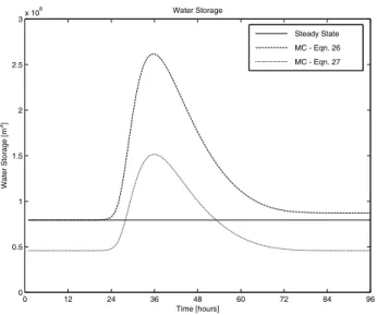
Water Storage
Steady State MC - Eqn. 26 MC - Eqn. 27
Fig. 1. Steady state volume (solid line) and storage volumes com-puted using Eq. (26) (dashed line) and Eq. (27) (dotted line).
Therefore, by imposing that the numerical diffusion equals the physical one (see also Sz´el and G´asp´ar, 2000; Wang et al., 2006), Cunge (1969) derived an expression forε.
ε= 1
2
1−c1xBSQ
0
(22)
which was used, together withk=1xc in Eq. (18), and up-dated at each time step, to give rise to the so called Variable Parameter Muskingum-Cunge approach. Successively, with-out changing the nature of the problem, Ponce and Yevjevich proposed (1978) the following expressions forC1,C2,C3:
C1=−
1+C+D
1+C+D ; C2=
1+C−D
1+C+D; C3=
1−C+D
1+C+D (23)
derived in terms of the dimensionless “Courant number”(C); and “cell Reynolds number”(D), which is the ratio of the physical and numerical diffusivities
C= c1t
1x; D=
Q B S0c 1x
(24) Several ways for estimatingQandchave been also proposed in the literature (Ponce and Chaganti, 1994; Tang et al., 1999; Wang et al., 2006) giving rise to a wide variety of three or four point schemes.
ParametersCandDare generally estimated, at each time interval, as a function of a reference dischargeQrelevant to each computation section in which a river reach will be di-vided. This poses certain limitations on the length1xof the computation section. Q,which will be evaluated at a cen-tral point, will be used to estimate the water stage and the other quantities of interest such asB,c and finally C and
D. The larger1x is, the likelihood that the Muskingum hy-pothesis on the linear variation in space of the discharge will
hold, decreases. Although, this property is also influenced by bed slope, friction and surface width, as a rule of thumb one should never exceed few kilometers (possibly one) to avoid errors which will be more evident in terms of water stage.
By comparing Eq. (10) and Eq. (23) one can finally derive the expressions for the two original Muskingum parameters:
k= 1tC ε= 1−2D
(25a) (25b) The model with the two parameters estimated in every computation section of length1x and at each time step1t
according to Eqs. (25) is known as the Muskingum-Cunge (MC) method and has been, and still is, widely used all over the world for routing discharges.
Unfortunately two inconsistencies have been detected in the practical use of MC. The first one, which relates to a loss of mass was identified by several authors and widely reported (see for instance Ponce and Yevjevich, 1978; Koussis, 1983; Ponce and Chaganti, 1994; Tang et al., 1999, Perumal et al., 2001) and recently interpreted as inversely proportional to the bed slope (Tang et al., 1999).
The second one, relates to the fact that if one discretises Eq. (1a), to estimate the storage in the reach, one obtains:
St+1t =St+
I
t+1t +It
2 −
Ot+1t+Ot
2
1t (26)
The same storage can also be estimated by discretising Eq. (1b) and using the values fork andεdetermined from Eqs. (25), which gives:
St+1t =k ε It+1t +k (1−ε) Ot+1t (27)
Astonishingly, no one seems to have checked back the ef-fect of the Cunge variable parameter estimation on the two Muskingum basic equations. Paradoxically, not only do the two equations lead to different results, but neither of them is even consistent with the steady state conditions.
Without loss of generality, Fig. 1 shows the storage val-ues, computed from Eqs. (26) and (27), for the base case with rectangular cross-section, which is described in the “Numer-ical experiment” section. From the figure, one can notice that (i) the stored volume computed using Eq. (26) does not return to the original steady state as a consequence of the above mentioned mass balance inconsistency (in practice the water is not lost, but rather stored in the channel reach) and (ii) Eq. (27) produces a storage which is always lower than it should be. In particular, the analysis of the steady state, namely when the inflow and outflow discharges are identical and Eq. (27) degenerates intoSt+1t=k It+1t =k Ot+1t,
re-veals that this effect can only be attributed to a wrong value estimated for parameterk.
3 Resolving the mass conservation inconsistency
Several authors (Ponce and Yevjevich, 1978; Koussis, 1980; Ponce and Chaganti, 1994; Tang et al. 1999, Perumal et al., 2001) have reported that while the original constant pa-rameter Muskingum perfectly preserves mass balance, the variable parameter Muskingum-Cunge suffers from a loss of mass which increases with the flatness of the bed slope, reaching values of the order of 8 to 10% at slopes of the or-der of 10-4(Tang et al. 1999).
Most of the above mentioned authors have tried to find alternative numerical schemes to improve the conservation of mass (or continuity), but no real explanation was ever given for the causes of this loss of mass, since they did not realize that the actual reason was hidden in the original derivation of the Muskingum equation.
It is interesting to notice that the seed for the modifica-tion proposed in this paper can also be found in a comment by Cunge (2001). As can be seen in his comment, Cunge attributes the non-conservation mass to an inaccurate dis-cretization by Tang et al. (1999), which, on the other hand is fully consistent with the Muskingum model formulation given by Eq. (3). Cunge does not seem to realize that the jus-tification for the different discretization he proposes lies in a different derivation of the Muskingum model, which allows from the very beginning for the possibility of time variant parameters.
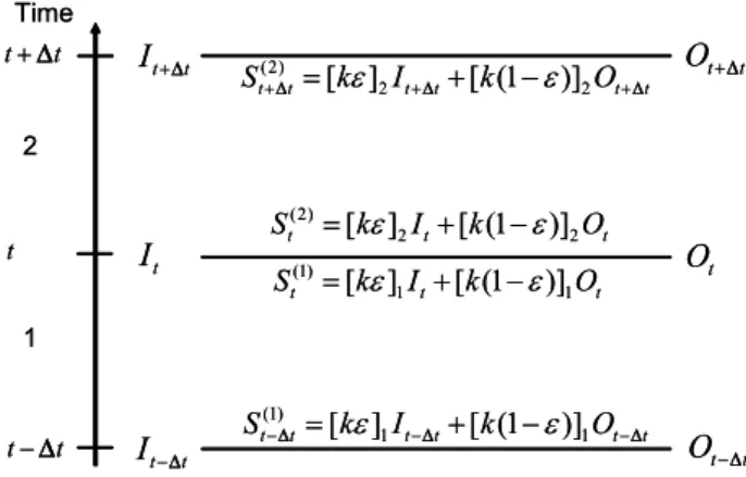
Not enough attention has been paid to the fact that the orig-inal derivation of the Muskingum approach “implies” time constant parameters with the consequence that Eq. (3) is only valid ifkandεare constant in time, which justifies the use of average values within a time interval as in Tang et al. (1999) and in most of the cited works. If one discretises Eq. (3), as was done to derive Eq. (5), it is quite evident that one is supposed to use constantk andε in each time-step which creates the situation illustrated in Fig. 2. As can be seen in the figure, at the boundary between of two time steps (time step 1 between timest−1t andt and time step 2 between timest andt+1t) the inflow and outflow discharges,It and Otare the same in both time steps. However, this is not true
for the volume stored in the reach, because of the following inequality:
St(2)=[kε]2It +[k (1−ε)]2Ot 6=St(1)
=[kε]1It+[k (1−ε)]1Ot (28)
since [kε]1 and [k (1−ε)]1, the average parameter values in time step 1 are not constrained to be equal to [kε]2 and [k (1−ε)]2, the average parameter values in time step 2. This will result in a difference that will accumulate over time with the consequent mass conservation inconsistency.
On the contrary, if one assumes that k andε may vary in time, Eq. (3) is no longer valid and one has to directly
t t−Δ t
t t+Δ
t t
O−Δ
t t
I−Δ
t
I
t t
I+Δ
t
O
t t
O+Δ
t t t
t t
t k I k O
S+Δ = +Δ + − +Δ
2 2
) 2
( [ ε] [ (1 ε)]
t t t
t t
t k I k O
S−Δ = −Δ + − −Δ
1 1 ) 1 ( )] 1 ( [ ]
[ ε ε
t t
t k I k O
S 1 1 ) 1 ( )] 1 ( [ ]
[ ε + −ε
=
t t
t k I k O
S(2) 2 2
)] 1 ( [ ]
[ ε + −ε
= Time
1 2
t t−Δ t
t t+Δ
t t
O−Δ
t t
I−Δ
t
I
t t
I+Δ
t
O
t t
O+Δ
t t t
t t
t k I k O
S+Δ = +Δ + − +Δ
2 2
) 2
( [ ε] [ (1 ε)]
t t t
t t
t k I k O
S−Δ = −Δ + − −Δ
1 1 ) 1 ( )] 1 ( [ ]
[ ε ε
t t
t k I k O
S 1 1 ) 1 ( )] 1 ( [ ]
[ ε + −ε
=
t t
t k I k O
S(2) 2 2
)] 1 ( [ ]
[ ε + −ε
= Time
1 2
Fig. 2.Storage values computed in two successive time steps. When using variable Muskingum-Cunge parameters, the storage valueSt
computed at time step 1 (St(1)) will differ from the one computed at time step 2 (St(2)), according to Eq. (28).
discretise Eq. (2), using the following definitions:
I ≃ It+1t+It
2 ; O ≃
Ot+1t +Ot
2 ;
d [k ε I]
dt
≃ 1 [1tk ε I] =[kε]t+1tIt1t+1t −[kε]tIt;d [k (1dt−ε) O] ≃1 [k (1−ε) O]
1t =
[k (1−ε)]t+1t Ot+1t−[k (1−ε)]t Ot 1t
(29) Note that the quantities [kε] and [k (1−ε)] appearing in Eqs. (28) and (29) are put in square brackets to mark that in the sequel these, and not the originalkandε, used in the steady-state Muskingum equations, will be considered as the actual time varying model parameters. Appendix A demon-strates the validity of the approximation implied in Eq. (29). Substitution of the quantities defined in Eq. (29) into Eq. (2) yields:
[kε]t+1tIt+1t−[kε]tIt
1t +
[k (1−ε)]t+1t Ot+1t−[k (1−ε)]t Ot
1t
= It+1t+It
2 −
Ot+1t+Ot
2 (30)
as the valid time varying finite difference approximation for the variable parameter Muskingum approach.
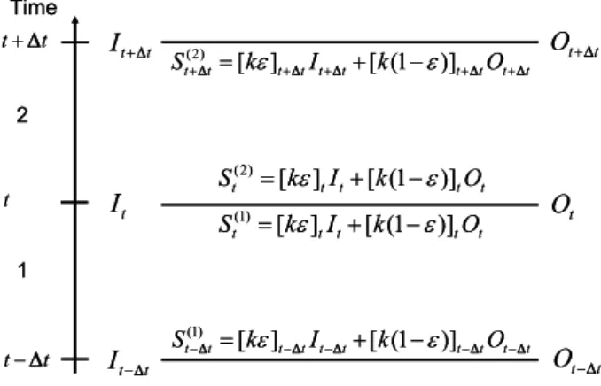
As can be seen from Fig. 3, not only the inflow and outflow discharges are now equal at the boundary between two time steps, but also the volumes stored in the reach at that instant are the same when computed in either interval:
St(2)=[kε]tIt+[k (1−ε)]tOt=S(t1)=[kε]tIt+[k (1−ε)]tOt
(31) By multiplying both sides of Eq. (30) by 21t the following expression is obtained:
2 [kε]t+1tIt+1t−2 [kε]tIt+2 [k (1−ε)]t+1tOt+1t−2 [k (1−ε)]tOt
=1t (It+1t+It)−1t Ot+1t+Ot
t t−Δ t
t t+Δ
t t
O−Δ
t t
I−Δ
t
I
t t
I+Δ
t
O
t t
O+Δ
t t t t t t t t t
t k I k O
S(+2Δ) =[ ε]+Δ +Δ +[ (1−ε)]+Δ +Δ
t t t t t t t t t
t k I k O
S(−1)Δ =[ ε]−Δ −Δ +[ (1−ε)]−Δ −Δ t t t
t
t k I k O
S(1)=[ ε] +[ (1−ε)]
t t t
t
t k I k O
S(2)=[ ε] +[ (1−ε)]
Time
1 2
t t−Δ t
t t+Δ
t t
O−Δ
t t
I−Δ
t
I
t t
I+Δ
t
O
t t
O+Δ
t t t t t t t t t
t k I k O
S(+2Δ) =[ ε]+Δ +Δ +[ (1−ε)]+Δ +Δ
t t t t t t t t t
t k I k O
S(−1)Δ =[ ε]−Δ −Δ +[ (1−ε)]−Δ −Δ t t t
t
t k I k O
S(1)=[ ε] +[ (1−ε)]
t t t
t
t k I k O
S(2)=[ ε] +[ (1−ε)]
Time
1 2
Fig. 3.Storage values computed in two successive time steps. When using variable Muskingum-Cunge parameters with the proposed correction, the storage valueSt computed at time step 1 (St(1)) will
equal the one computed at time step 2 (St(2)), according to Eq. (31).
which can be rewritten as:
2 [k (1−ε)]t+1t+1t Ot+1t=−2 [kε]t+1t+1t It+1t
+ {2 [kε]t+1t} It+
2 [k (1−ε)]t−1t Ot (33)
to give:
Ot+1t= −
2 [kε]t+1t+1t
2 [k (1−ε)]t+1t +1t It+1t
+ 2 [kε]t+1t
2 [k (1−ε)]t+1t+1t It+
2 [k (1−ε)]t−1t
2 [k (1−ε)]t+1t+1t Ot(34)
Finally, Eq. (34) can be rewritten as:
Ot+1t =C1It+1t+C2It+C3Ot (35)
with the following substitutions:
C1= −
2[kε]t+1t+1t
2 [k (1−ε)]t+1t +1t; C2=
2[kε]t+1t
2 [k (1−ε)]t+1t +1t; C3=
2 [k (1−ε)]t−1t
2 [k (1−ε)]t+1t+1t
(36) whereC1, C2andC3are the three coefficients that still guar-antee the property expressed by Eq. (11). The same parame-ters can also be obtained in terms of the Courant number and of the cell Reynolds number:
C1=−
1+Ct+1t+Dt+1t
1+Ct+1t+Dt+1t ; C2=
1+Ct−Dt
1+Ct+1t+Dt+1t Ct+1t
Ct ;
C3=
1−Ct +Dt
1+Ct+1t +Dt+1t Ct+1t
Ct
(37) after substituting for:
(
[kε]t+1t =
(1−Dt+1t)1t
2Ct+1t ; [kε]t =
(1−Dt)1t
2Ct
[k (1−ε)]t+1t =
(1+Dt+1t)1t
2Ct+1t ;[k (1−ε)]t =
(1+Dt)1t
2Ct
(38)
This scheme is now mass conservative, but there is still an inconsistency between Eqs. (26) and (27).
To elaborate: Eq. (26) now leads to a storageStthat is
con-sistent with the steady state, both at the beginning and at the end of a transient; however, Eq. (27) produces a result which is always different from the one produced by Eq. (26) and, in addition, is also not consistent with the expected steady state storage in the channel.
4 Resolving the steady state inconsistency
In order to resolve the steady state inconsistency, one needs to look in more detail into Eq. (27). If one substitutes for [kε] and [k(1−ε)], given by Eqs. (25), into Eq. (27) written for a generic timet(which is omitted for the sake of clarity), one obtains:
S= 1t C
1−D
2 I+
1t C
1+D
2 O (39)
which can be re-arranged as:
S= 1t C
O+I
2 +
1t D C
O−I
2 (40)
Clearly, 1tC O+2I, the first right hand side term in Eq. (40), represents the storage at steady state, since the second term vanishes due to the fact that the steady state is characterised byI=O. Consequently,1t DC O2−I, the second right hand side term in Eq. (40), can be considered as the one governing the unsteady state dynamics.
In the case of steady flow, whenI=O=O+2I=Q, under the classical assumptions of the Muskingum model, together with the definition of discharge Q=Av, withAthe wetted area[L2], and v the velocity [LT−1], the following result can be obtained for the storage:
S=A1x= Q
v1x =k
∗Q (41)
with1x the length of the computational interval [L], and
k∗=1xv [T]the resulting steady state parameter, which can be interpreted as the time taken for a parcel of water to tra-verse the reach, as distinct from the kinematic celerity or wave speed.
It is not difficult to show thatk∗6=k. By substituting forC
given by Eq. (24) into Eq. (25a) one obtains the inequality:
k=1x
c 6= 1x
v =k
∗ (42)
Therefore, if one wants to be consistent with the steady state specialization of the Muskingum model, one needs to usek∗ instead ofk. This can be easily done by defining a dimensionless correction coefficientβ=c/vand by dividing
Cbyβ,C∗=C/β= v1t1xso thatk∗=1tC∗=1xv .
This correction satisfies the steady state, but inevitably modifies the unsteady state dynamics, since the coefficient of the second right hand side term in Eq. (40) now becomes
1t D
C∗ . It is therefore necessary to defineD∗=D/βso that: 1t D∗
C∗ =
1t D
C (43)
By incorporating these results, Eq. (38) can finally be rewrit-ten as:
[kε]t+1t =
1−D∗t+1t
1t
2C∗t+1t ; [kε]t =
(1−Dt∗)1t
2C∗t
[k (1−ε)]t+1t =
1+Dt∗+1t
1t
2Ct∗+1t ;[k (1−ε)]t =
(1+Dt∗)1t
2C∗t
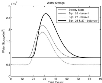
(44) These modifications do not alter the overall model dynamics, but allow Eq. (27) to satisfy the steady state condition. Fig-ure 4 shows the results of the proposed modifications. The storage derived with Eq. (27) is now identical to the one pro-duced by Eq. (26) and they both comply with the steady state condition.
As a final remark, please note that, the parameterεis al-lowed to take negative values that are legitimate in the vari-able parameter approaches such as the MC and the newly proposed one, without inducing neither numerical instability nor inaccuracy in the results, as demonstrated by Sz´el and G´asp´ar (2000).
5 The new mass conservative and steady state consistent variable parameter Muskingum-Cunge method
The formulation of the new algorithm, which will be referred in this paper as the variable parameter Muskingum-Cunge-Todini (MCT) method, is provided here for a generic cross section, which is assumed constant in space within a single reach.
A first guess estimateOˆt+1tfor the outflowOt+1tat time t+1tis initially computed as:
ˆ
Ot+1t =Ot +(It+1t −It) (45)
Then the reference discharge is computed at times t and
t+1tas:
Qt = It +Ot
2 (46a)
Qt+1t =
It+1t + ˆOt+1t
2 (46b)
0 12 24 36 48 60 72 84 96
0 0.5 1 1.5 2 2.5
3x 10 6
Time [hours]
Water Storage [m
3]
Water Storage
Steady State Eqn. 26 - beta=1 Eqn. 27 - beta=1 Eqn. 26 & 27 - beta=c/v
Fig. 4. Steady state volume (thin solid line) and storage volumes computed either using Eq. (26) (dashed line) and Eq. (27) (dotted line) withβ=1, or using both equations withβ=c/v(thick solid line).
where the reference water levels can be derived by means of a Newton-Raphson approach from the following implicit equations:
yt =y{Qt, n, S0} (47a)
yt+1t =y{Qt+1t, n, S0} (47b)
Details of the Newton-Raphson procedure can be found in Appendix B.
Using the reference discharge and water level it is then possible to estimate all the other quantities at timest and
t+1t.
The celerityc:
ct =c{Qt, yt, n, S0} (48a)
ct+1t =c{Qt+1t, yt+1t, n, S0} (48b) Note: the actual expressions for the celerity valid for trian-gular, rectangular and trapezoidal cross sections, are given in Appendix C.
The specialization of other necessary parameters follows. The correcting factorβ:
βt = ctAt
Qt
(49a)
βt+1t =
ct+1t At+1t Qt+1t
The corrected Courant numberC∗:
Ct∗= ct βt
1t
1x (50a)
Ct∗+1t = ct+1t βt+1t
1t
1x (50b)
and the corrected cell Reynolds numberD∗:
D∗t = Qt
βtBS0ct1x
(51a)
D∗t+1t = Qt+1t βt+1tBS0ct+1t1x
(51b) Finally the MCT parameters are expressed as:
C1= −
1+Ct∗+D∗t
1+Ct∗+1t+Dt∗+1t; C2=
1+Ct∗−Dt∗
1+Ct∗+1t+D∗t+1t Ct∗+1t
Ct∗ ;
C3=
1−Ct∗+Dt∗
1+Ct∗+1t+Dt∗+1t Ct∗+1t
Ct∗ (52)
which yields the estimation of the flow at timet+1tthrough the standard formulation:
ˆ
Ot+1t =C1It+1t+C2It+C3Ot (53)
Note that while it is advisable to repeat twice the computa-tions of Eqs. (46b), (47b), (48b), (49b), (50b), (51b), (52) and (53), in order to eliminate the influence of the first guess
ˆ
Ot+1t given by Eq. (45), it is only necessary to compute
Eqs. (46a), (47a), (48a), (49a), (50a), (51a) once at timet=0, since fort >0 one can use the value estimated at the previ-ous time step .
OnceOˆt+1tis known, one can estimate the storage at time t+1tas
St+1t =
1−Dt∗+1t1t
2Ct∗+1t It+1t +
1+Dt∗+1t1t
2Ct∗+1t Ot+1t
(54) by substituting for [kε] and [k(1−ε)] given by Eqs. (44) into Eq. (27) and by settingOt+1t= ˆOt+1t.
Eventually, the water stage can be estimated, by taking into account that the Muskingum model is a lumped model in space, which means that the water level will represent the “average” water level in the reach. This differs from the estimation of the water stage proposed by Ponce and Lugo (2001) since they incorporate the estimation of the wa-ter stage in the four points scheme used to solve the kine-matic/parabolic interpretation of the Muskingum equation, which is not a lumped model.
Therefore, taking into account the lumped nature of the MCT equation, one can estimate the average wetted area in the river reach:
¯
At+1t= St1x+1t (55)
from which, knowing the shape of the cross section, the water stage can be evaluated:
yt+1t =yA¯t+1t (56)
Equation (56) represents the average water stage in the reach and, on the basis of the Muskingum wedge assumption can be interpreted as the water stage more or less in the centre of the reach. This should not be considered as a problem, given that most of the classical models (see for instance MIKE11 – DHI Water & Environment, 2000) in order to produce mass conservative schemes (Patankar, 1980), correctly discretise the full de Saint Venant equations using alternated grid points where the water stage (potential energy) and flow (kinetic energy) are alternatively computed along the river.
6 The role of the “pressure term”
Cappelaere (1997), discussed the advantages of an accurate diffusive wave routing procedure and the possibility of intro-ducing a “pressure correcting term” to improve its accuracy. He also acknowledged the fact that variable parameter Ad-vection Diffusion Equation (ADE) models (Price, 1973; Boc-quillon and Moussa, 1988) do not guarantee mass conserva-tion. He concludes by stating that the introduction of the pressure term “increasing model compliance with the funda-mental de Saint Venant equations guarantees that the basic principles of momentum and mass conservation are better satisfied...”.
In reality, because the proposed MCT is mass conserva-tive, the introduction of the pressure term correction has no effect on mass conservation. Nonetheless, the introduction of the pressure correction term, on the basis that the parabolic approximation uses the water surface slope instead of the bottom slope to approximate the head slope, certainly im-proves the dynamical behaviour of the algorithm. This will be shown in the sequel through a numerical example.
7 Numerical example
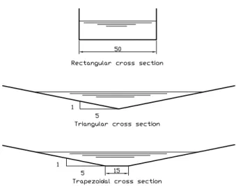
In this study, in addition to the basic channels adopted in the Flood Studies Report (FSR) (NERC 1975), namely a rectan-gular channel (with a widthB=50 m, a Manning’s coefficient
n=0.035, and a total channel lengthL=100 km, but with dif-ferent bed slopes S0 ranging from 10−3 to 10−4), a trian-gular and a trapezoidal channel were also analysed. Both the triangular and the trapezoidal channels are supposed to be contained by dykes with a slope ratio (elevation/width) tan(α)=1/5 while the trapezoidal channels have a bottom widthB0=15 m (Fig. 5).
A synthetic inflow hydrograph (NERC 1975) was defined as
Q (t )=Qbase+ Qpeak−Qbase
t
Tp
exp
1− t
Tp
β
Table 1. Variation of parameters and integration steps around the base case (in bold).
So 0.002 0.001 0.0005 0.00025 0.0001
n 0.01 0.02 0.035 0.04 0.06
1x 1000 2000 4000 6000 8000
1t 900 1800 3600 5400 7200
where β=16; Qpeak=900 m3s−1; Qbase=100m3s−1; and
Tp=24 h.
For each cross section (rectangular, triangular and trape-zoidal) a reference run was defined with the following pa-rameters:
S0=0.00025
n=0.035 m−1/3s
1x=2000 m
1t=1800 s
In addition, each parameter was perturbed, as in Table 1, in order to analyse its effect on the preservation of the volume, the peak flow and relevant time of occurrence, the peak level and relevant time of occurrence.
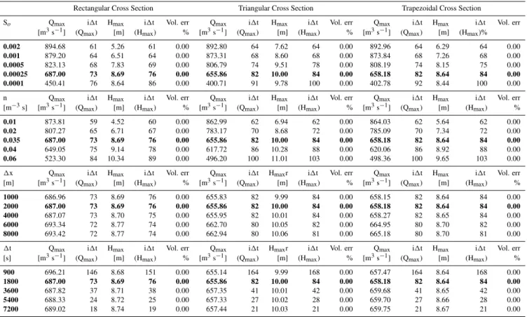
The results of the experiment are given in Table 2, when the MCT is used without Cappelaere (1997) proposed cor-rection and in Table 3 when the corcor-rection is applied.
The tables are divided into three columns representing the different cross sections used and in four rows relevant to the variation of bottom slope (S0), friction (n), space integration interval (1x) and time integration interval (1t).
As one can see from Table 2, as opposed to the incomplete effectiveness of empirical corrections, such as the one pro-posed by Tang et al. (1999), when using the MCT approach thevolume error remains equal to zero in all the examined cases independently from the variation of bottom slope, fric-tion, space and time integration intervals and Cappelaere cor-rection. Moreover, Table 3 shows that this is also true when this correction is applied.
In particular, Tables 2 and 3 one should note that the ef-fect induced by the variation of the bed slope and the friction coefficient is always consistent with that expected. More in-teresting is the fact that relatively small effects on the peak flow and its time of occurrence, as well as on the peak level and the time of its occurrence, are produced by the variation of the integration time and space steps.
Nonetheless, one should realize that in the numerical ex-ample, the bottom slope, the shape of the channel, the fric-tion, etc. are constant, which is not the case in real rivers, where the bottom slope and the cross section shape and all the other characteristics change continuously. Given the wide number of different cases, there is no unique rule, but in real world application one must divide a river reach into a number
Fig. 5.The three cross sections shapes (rectangular, triangular and trapezoidal) and the relevant dimensions used in the numerical ex-periment.
of computation sections of limited length, for which the hy-pothesis of constant bed slope, shape and friction, as well as linear variation of the discharge, required by the Muskingum approach, is a consistent approximation. On the same lines, the integration time interval must be sufficiently small to al-low the user to correctly represent the peak fal-low and stage in terms of magnitude (they obviously become smoothed if the time-step is too long) and time of occurrence.
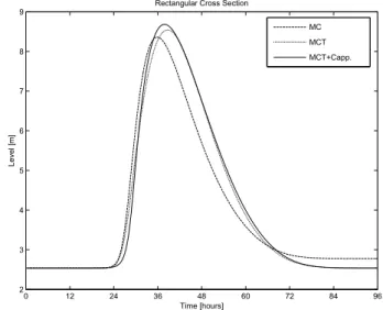
Figures 6 and 7, which were derived using the reference run parameters, show the behaviour of the original variable parameter Muskingum-Cunge (MC) approach when com-pared to the MCT and the MCT with the Cappelaere correc-tion (MCT+C), for the base case applied to the rectangular channel. It is easy to note from Figure 6 that the MC peak discharge is anticipated and much higher than the ones pro-duced by the MCT and the MCT+C. Moreover Fig. 7 shows how the MC water level, as opposed to the ones produced by MCT and MCT+C, does not return to the steady state at the end of the transient.
Finally to understand the hydraulic improvement obtained by the MCT and the MCT+C, their results were compared to the ones produced using a full de Saint Venant approach (MIKE11 – DHI Water & Environment, 2000).
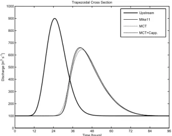
Figures 8 and 9 show the results in terms of discharge and water levels for the rectangular cross section; Figs. 10 and 11 show the results for the triangular cross section; and Figs. 12 and 13 show the results for the trapezoidal cross section. In the case of the rectangular section the results of the MCT+C perfectly match the results of MIKE11, while in the case of the triangular and the trapezoidal cross sections, the re-sults, although not perfectly matching the ones produced by MIKE11, are very good approximations.
Table 2.Variation of MCT results without Cappalaere (1997) proposed correction. Base case in bold.
Rectangular Cross Section Triangular Cross Section Trapezoidal Cross Section
So Qmax i1t Hmax i1t Vol. err Qmax i1t Hmax i1t Vol. err Qmax i1t Hmax i1t Vol. err [m3s−1] (Qmax) [m] (Hmax) % [m3s−1] (Qmax) [m] (Hmax) % [m3s−1] (Qmax) [m] (Hmax)%
0.002 894.68 61 5.26 61 0.00 892.80 64 7.62 64 0.00 892.95 64 6.29 64 0.00
0.001 879.10 64 6.51 64 0.00 873.11 68 8.60 68 0.00 873.65 68 7.26 68 0.00
0.0005 819.78 68 7.81 69 0.00 802.64 74 9.49 75 0.00 804.27 74 8.14 75 0.00
0.00025 669.53 75 8.54 77 0.00 641.17 83 9.91 86 0.00 643.74 83 8.56 86 0.00
0.0001 423.11 77 8.32 89 0.00 391.80 93 9.70 103 0.00 393.72 93 8.36 103 0.00
n Qmax i1t Hmax i1t Vol. err Qmax i1t Hmax i1t Vol. err Qmax i1t Hmax i1t Vol. err
[m−3s] [m3s−1] (Qmax) [m] (Hmax) % [m3s−1] (Qmax) [m] (Hmax) % [m3s−1] (Qmax) [m] (Hmax) %
0.01 873.19 59 4.52 60 0.00 862.15 62 6.94 62 0.00 863.26 62 5.63 62 0.00
0.02 801.63 66 6.67 67 0.00 776.52 71 8.65 72 0.00 778.72 71 7.31 72 0.00
0.035 669.53 75 8.54 77 0.00 641.17 83 9.91 86 0.00 643.74 83 8.56 86 0.00
0.04 630.09 77 8.96 80 0.00 603.12 87 10.18 90 0.00 605.61 87 8.83 90 0.00
0.06 505.99 87 10.12 92 0.00 486.19 102 10.92 106 0.00 488.26 102 9.56 106 0.00
1x Qmax i1t Hmax i1t Vol. err Qmax i1t Hmaxr i1t Vol. err Qmax i1t Hmax i1t Vol. err [m] [m3s−1] (Qmax) [m] (Hmax) % [m3s−1] (Qmax) [m] (Hmax) % [m3s−1] (Qmax) [m] (Hmax) %
1000 669.51 75 8.54 77 0.00 641.12 83 9.91 86 0.00 643.69 83 8.56 86 0.00
2000 669.53 75 8.54 77 0.00 641.17 83 9.91 86 0.00 643.74 83 8.56 86 0.00
4000 669.62 75 8.56 77 0.00 641.38 83 9.92 85 0.00 643.94 83 8.57 85 0.00
6000 675.69 74 8.62 76 0.00 648.35 82 9.97 83 0.00 650.83 82 8.61 83 0.00
8000 675.92 73 8.63 75 0.00 648.75 82 9.98 83 0.00 651.22 82 8.62 83 0.00
1t Qmax i1t Hmax i1t Vol. err Qmax i1t Hmaxr i1t Vol. err Qmax i1t Hmax i1t Vol. err
[s] [m3s−1] (Qmax) [m] (Hmax) % [m3s−1] (Qmax) [m] (Hmax) % [m3s−1] (Qmax) [m] (Hmax) %
900 669.65 149 8.54 155 0.00 641.36 167 9.91 171 0.00 643.89 167 8.56 171 0.00
1800 669.53 75 8.54 77 0.00 641.17 83 9.91 86 0.00 643.74 83 8.56 86 0.00
3600 669.15 37 8.54 39 0.00 641.16 42 9.91 43 0.00 643.68 42 8.56 43 0.00
5400 669.55 25 8.54 26 0.00 641.25 28 9.91 29 0.00 643.79 28 8.56 29 0.00
7200 668.43 19 8.52 19 0.00 641.28 21 9.90 22 0.00 643.86 21 8.54 22 0.00
0 12 24 36 48 60 72 84 96
0 100 200 300 400 500 600 700 800
Time [hours]
Discharge [m
3 s -1]
Rectangular Cross Section
MC
MCT
MCT+Capp.
Fig. 6.Comparison of the discharge results obtained using the vari-able parameter Muskingum-Cunge (dashed line), the new scheme (dotted line) and the new scheme with the Cappelaere (1997) cor-rection (solid line).
0 12 24 36 48 60 72 84 96
2 3 4 5 6 7 8 9
Time [hours]
Level [m]
Rectangular Cross Section
MC
MCT
MCT+Capp.
Table 3.Variation of MCT results with Cappalaere (1997) proposed correction. Base case in bold.
Rectangular Cross Section Triangular Cross Section Trapezoidal Cross Section
So Qmax i1t Hmax i1t Vol. err Qmax i1t Hmax i1t Vol. err Qmax i1t Hmax i1t Vol. err [m3s−1] (Qmax) [m] (Hmax) % [m3s−1] (Qmax) [m] (Hmax) % [m3s−1] (Qmax) [m] (Hmax)%
0.002 894.68 61 5.26 61 0.00 892.80 64 7.62 64 0.00 892.96 64 6.29 64 0.00
0.001 879.20 64 6.51 64 0.00 873.31 68 8.60 68 0.00 873.84 68 7.26 68 0.00
0.0005 823.13 68 7.83 69 0.00 806.79 74 9.51 78 0.00 808.19 74 8.15 75 0.00
0.00025 687.00 73 8.69 76 0.00 655.86 82 10.00 84 0.00 658.18 82 8.64 84 0.00
0.0001 450.41 76 8.64 86 0.00 400.71 91 9.78 100 0.00 402.78 92 8.44 100 0.00
n Qmax i1t Hmax i1t Vol. err Qmax i1t Hmax i1t Vol. err Qmax i1t Hmax i1t Vol. err
[m−3s] [m3s−1] (Qmax) [m] (Hmax) % [m3s−1] (Qmax) [m] (Hmax) % [m3s−1] (Qmax) [m] (Hmax) %
0.01 873.81 59 4.52 60 0.00 862.99 62 6.94 62 0.00 864.03 62 5.64 62 0.00
0.02 807.27 65 6.71 67 0.00 783.17 70 8.68 72 0.00 785.09 70 7.34 72 0.00
0.035 687.00 73 8.69 76 0.00 655.86 82 10.00 84 0.00 658.18 82 8.64 84 0.00
0.04 649.05 75 9.14 78 0.00 617.72 86 10.28 88 0.00 620.06 86 8.92 88 0.00
0.06 523.30 84 10.34 89 0.00 496.20 100 11.01 103 0.00 498.36 100 9.65 103 0.00
1x Qmax i1t Hmax i1t Vol. err Qmax i1t Hmaxr i1t Vol. err Qmax i1t Hmax i1t Vol. err [m] [m3s−1] (Qmax) [m] (Hmax) % [m3s−1] (Qmax) [m] (Hmax) % [m3s−1] (Qmax) [m] (Hmax) %
1000 686.96 73 8.69 76 0.00 655.83 82 9.99 84 0.00 658.15 82 8.64 84 0.00
2000 687.00 73 8.69 76 0.00 655.86 82 10.00 84 0.00 658.18 82 8.64 84 0.00
4000 687.07 73 8.70 75 0.00 655.95 82 10.01 84 0.00 658.27 82 8.65 84 0.00
6000 693.34 72 8.77 74 0.00 662.70 80 10.05 82 0.00 664.95 80 8.70 82 0.00
8000 693.42 72 8.77 74 0.00 662.94 80 10.06 81 0.00 665.18 80 8.70 81 0.00
1t Qmax i1t Hmax i1t Vol. err Qmax i1t Hmaxr i1t Vol. err Qmax i1t Hmax i1t Vol. err
[s] [m3s−1] (Qmax) [m] (Hmax) % [m3s−1] (Qmax) [m] (Hmax) % [m3s−1] (Qmax) [m] (Hmax) %
900 696.21 146 8.68 151 0.00 655.14 164 9.99 168 0.00 657.47 164 8.64 168 0.00
1800 687.00 73 8.69 76 0.00 655.86 82 10.00 84 0.00 658.18 82 8.64 84 0.00
3600 687.82 37 8.71 38 0.00 657.35 41 10.01 42 0.00 659.68 41 8.65 42 0.00
5400 688.33 24 8.72 25 0.00 657.33 27 10.02 28 0.00 659.70 27 8.66 28 0.00
7200 689.02 18 8.74 19 0.00 657.44 21 10.03 21 0.00 659.75 21 8.67 21 0.00
wetted perimeter with respect to MIKE11, or (2) on the ex-tension of the Cappelaere correction to non rectangular chan-nels.
8 Conclusions
This paper deals with two inconsistencies deriving from the introduction, as proposed by Cunge (1969), of time variable parameters in the original Muskingum method. The first in-consistency relates to a mass balance error shown by the vari-able parameter MC method that can reach even values of 8 to 10%. This incompatibility, has been widely reported in the literature and has been the objective of several tentative solutions, although a conclusive and convincing explanation has not been offered. In addition to the lack of mass balance, an even more important paradox is generated by the variable parameter MC approach, which apparently has never been reported in the literature. The paradox is: if one substitutes the parameters derived using Cunge approach back into the Muskingum equations, two different and inconsistent values for the water volume stored in the channel, are obtained.
This paper describes the analysis that was carried out, the explanation for the two inconsistencies and the corrections
that have been found to be appropriate. A new Muskingum algorithm, allowing for variable parameters, has been de-rived, which leads to slightly different equations from the original Muskingum-Cunge ones. The quality of the results has been assessed by routing a test wave (the asymmetri-cal wave proposed by Tang et al. (1999) already adopted in the Flood Studies Report (FSR, NERC 1975)), through three channels with different cross sections (rectangular, triangu-lar and trapezoidal), by varying the slope, the roughness, the space and time integration intervals. All the results obtained show that the new approach, in all cases, fully complies with the requirements of preserving mass balance, and at the same time satisfies the basic Muskingum equations. Finally, the ef-fect of the pressure term inclusion as proposed by Cappelaere (1997) was also tested. The results show an additional im-provement of the model dynamics when compared to the so-lutions using the full de Saint Venant equations, without any undesired effect on the mass balance and compliance with the Muskingum equations.
0 12 24 36 48 60 72 84 96 0
100 200 300 400 500 600 700 800 900 1000
Time [hours]
Discharge [m
3 s -1]
Rectangular Cross Section
Upstream Mike11 MCT MCT+Capp.
Fig. 8. Comparison, for the rectangular cross section, of the MIKE11 resulting discharges (thin solid line) with the ones ob-tained using the new MCT scheme (dotted line) and the new scheme with the Cappelaere (1997) correction (dashed line). The upstream inflow wave is shown as a thick solid line.
0 12 24 36 48 60 72 84 96
2 3 4 5 6 7 8 9 10 11
Time [hours]
Level [m]
Rectangular Cross Section
Upstream
Mike11
MCT
MCT+Capp.
Fig. 9. Comparison, for the rectangular cross section, of the MIKE11 resulting water stages (thin solid line) with the ones ob-tained using the new MCT scheme (dotted line) and the new scheme with the Cappelaere (1997) correction (dashed line). The upstream inflow wave is shown as a thick solid line.
models, which require, particularly in the routing compo-nent, the preservation of water balance to avoid compensat-ing it by adjustcompensat-ing other soil related parameter values. The proposed method will also be useful for routing flood waves in channels and in natural rivers with bottom slopes in the range of 10−3–10−4where the flood crest subsidence is one of the dominant phenomena. Within this range of slopes, the original MC approach was affected by the mass balance error which could be of the order of 10%.
0 12 24 36 48 60 72 84 96
0 100 200 300 400 500 600 700 800 900 1000
Time [hours]
Discharge [m
3 s -1]
Triangular Cross Section
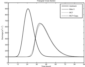
Upstream Mike11 MCT MCT+Capp.
Fig. 10. Comparison, for the triangular cross section, of the MIKE11 resulting discharges (thin solid line) with the ones ob-tained using the new MCT scheme (dotted line) and the new scheme with the Cappelaere (1997) correction (dashed line). The upstream inflow wave is shown as a thick solid line.
0 12 24 36 48 60 72 84 96
4 5 6 7 8 9 10 11 12
Time [hours]
Level [m]
Triangular Cross Section
Upstream
Mike11
MCT
MCT+Capp.
Fig. 11. Comparison, for the triangular cross section, of the MIKE11 resulting water stages (thin solid line) with the ones ob-tained using the new MCT scheme (dotted line) and the new scheme with the Cappelaere (1997) correction (dashed line). The upstream inflow wave is shown as a thick solid line.
0 12 24 36 48 60 72 84 96 0
100 200 300 400 500 600 700 800 900 1000
Time [hours]
Discharge [m
3 s -1]
Trapezoidal Cross Section
Upstream Mike11 MCT MCT+Capp.
Fig. 12. Comparison, for the trapezoidal cross section, of the MIKE11 resulting discharges (thin solid line) with the ones ob-tained using the new MCT scheme (dotted line) and the new scheme with the Cappelaere (1997) correction (dashed line). The upstream inflow wave is shown as a thick solid line.
0 12 24 36 48 60 72 84 96
3 4 5 6 7 8 9 10
Time [hours]
Level [m]
Trapezoidal Cross Section
Upstream
Mike11
MCT
MCT+Capp.
Fig. 13. Comparison, for the trapezoidal cross section, of the MIKE11 resulting water stages (thin solid line) with the ones ob-tained using the new MCT scheme (dotted line) and the new scheme with the Cappelaere (1997) correction (dashed line). The upstream inflow wave is shown as a thick solid line.
Appendix A
Proof thatat+1tbt+1t−atbt
1t is a consistent
discretiza-tion in time of d(ab)dt
In Eq. (29) the following two derivatives d[k ε Idt ] and
d[k (1−ε) O]
dt must be discretised in time. It is the scope of
this appendix to demonstrate that their discretization leads to
the expression used in Eqs. (29) and (30).
As can be noticed from Eqs. (10), the final Muskingum co-efficientsC1, C2, C3, do not directly depend on kandεtaken singularly, but rather on the two productsk εandk (1−ε). Therefore, both derivatives can be considered as the deriva-tives in time of a product of two termsaandb, beinga=k ε
andb=I in the first derivative anda=k (1−ε)andb =O
in the second one.
Expanding the derivatived(ab)dt one obtains:
d (ab)
dt =a
db dt +b
da
dt (A1)
which can be discretised in the time interval as follows:
1 (ab)
1t =
θ at+1t +(1−θ ) at
bt+1t −bt 1t
+
θ bt+1t+(1−θ ) bt
at+1t−at
1t (A2)
whereθis a non-negative weight falling in the range between 0 and 1. Since the Muskingum method is derived on the basis of a centered finite difference approach in time, this implies thatθ=12.
Therefore, Eq. (A2), becomes
1 (ab)
1t =
(at+1t+at)
2
bt+1t −bt
1t +
(bt+1t +bt)
2
at+1t−at 1t
= at+1tbt+1t +atbt+1t −at+1tbt−atbt
21t
+bt+1tat+1t+btat+1t −bt+1tat−btat
21t
= 2at+1tbt+1t−2btat
21t =
at+1tbt+1t−atbt
1t (A3)
Equation (A3) allows to write:
1 [k ε I]
1t =
[k ε]t+1tIt+1t−[k ε]tIt
1t (A4)
1 [k (1 − ε) O]
1t
= [k (1 − ε)]t+1t Ot+1t1t −[k (1 − ε)]t Ot (A5)
as they appear in Eqs. (29) and are then used in the derivation of the MCT algorithm.
Appendix B
The Newton-Raphson algorithm to derivey=y{Q, n, S0}
for a generic cross section
closed solution is not generally available, several numerical approaches to find the zeroes of a non-linear function can be used, such as the bisection or the Newton-Raphson ap-proaches.
In this case, given that the functions were continuous and differentiable (triangular, rectangular and trapezoidal cross sections), a simple Newton-Raphson algorithm was imple-mented. The problem is to find the zeroes of the following function ofy:
f (y)=Q (y)−Q=0 (B1)
where Q (y)L3T−1is defined as:
Q (y)=
√
S0
n
A (y)5/3
P (y)2/3 (B2)
with S0[dimensionless] the bottom slope, nL1/3T the Manning friction coefficient,A (y)L2the wetted area and
P (y)[L] the wetted perimeter, as defined in Appendix C. The Newton-Raphson algorithm, namely:
yi+1=yi−f (yi) /f′(yi) (B3)
allows one to find the solution to the problem with a limited number of iterations starting from an initial guessy0and can be implemented in this case by defining:
f (yi)=Q (yi)−Q=
√
S0
n
A (yi)5/3 P (yi)2/3
−Q (B4)
and
f′(yi)=
d[Q (y)−Q]
dy
y=yi
= dQ (y)dy
y=yi
(B5)
=5
3
√
S0
n
A (y)2/3 P (y)2/3
B (y)−4
5
A (y) P (y) sα
=B (y) c (y) (B6) using the results given in Appendix C.
Appendix C
The derivation ofA(h), B(h), c(h)andβ(h)for triangular, rectangular and trapezoidal cross sections
Given the cross-sections in Fig. 5, the following equations can be used to represent a generic triangular, rectangular or trapezoidal cross section.
A(y)=(B0+y cα) y (C1)
the wetted area
L2
B (y)=B0+2y cα (C2)
the surface width [L]
P (y)=B0+2y / sα (C3)
the wetted perimeter [L] with B0 the bottom width [L] (
B0=0 for the triangular cross section) andy the water stage [L]; cα=cot(α)andsα=sin(α)are respectively the
cotan-gent and the sine of the angleαformed by dykes over a hori-zontal plane (see Fig. 5) (cα=0 andsα=1 for the rectangular
cross section). Using these equations together with:
Q (y)=
√
S0
n
A (y)5/3
P (y)2/3 (C4)
the discharge
L3T−1
v (y)= Q (y) A (y) =
√
S0
n
A (y)2/3
P (y)2/3 (C5)
the velocityL T−1whereS0[dimensionless] is the bottom slope andn L1/3T the Manning friction coefficient, the celerity is calculated as:
c (y)= dQ (y) dA (y) =
1
B (y) dQ (y)
dy
= 5
3
√
S0
n
A (y)2/3 P (y)2/3
1−4
5
A (y)
B (y) P (y) sα
(C6) the celerity
L T−1
and the correction factor to be used in the MCT algorithm is:
β (y)= c (y) v (y) =
5 3
1−4
5
A (y) B (y) P (y) sα
(C7) the correction factor [dimensionless]
Edited by: E. Zehe
References
Bocquillon, C. and Moussa, R.: CMOD: Logiciel de choix de mod`eles d’ondes diffusantes et leur caract´eristique, La Houille Blanche, 5(6), 433–437 (in French), 1988.
Cappelaere, B.: Accurate Diffusive Wave Routing, J. Hydraulic Eng., ASCE, 123(3),174–181, 1997.
Chow, V. T.: Handbook of Applied Hydrology, McGraw-Hill, New York, NY, 1964.
Chow, V. T., Maidment, D. R., and Mays, L. W.: Applied Hydrol-ogy, McGraw-Hill, New York, NY, 1988
Cunge, J. A.: On the subject of a flood propagation computation method (Muskingum method), Delft, The Netherlands, J. Hydr. Res., 7(2), 205–230, 1969.
Cunge, J.: Volume conservation in variable parameter Muskingum-Cunge method – Discussion, J. Hydraul. Eng., ASCE, 127(3), 239–239, 2001.
DHI Water and Environment: MIKE 11, User Guide and Reference Manual, DHI Water & Environment, Horsholm, Denmark, 2000. Dooge, J. C. I.: Linear Theory of Hydrologic Systems, USDA Tech. Bull. 1468. US Department of Agriculture, Washington, D.C., 1973.
Kalinin, G. P. and Miljukov, P. I.: Approximate methods for com-puting unsteady flow movement of water masses. Transactions, Central Forecasting Institute. Issue 66 (in Russian, 1958). Koussis, A. D.: Comparison of Muskingum method difference
scheme Journal of Hydraulic Division, ASCE, 106(5), 925–929, 1980.
Koussis, A. D.: Accuracy criteria in diffusion routing: a discussion. Journal of Hydraulic Division, ASCE, 109(5), 803–806, 1983. Liu Z. and Todini E.: Towards a comprehensive physically based
rainfall-runoff model, Hydrol. Earth Syst. Sci., 6(5), 859–881, 2002.
Liu, Z. and Todini, E.: Assessing the TOPKAPI non-linear reser-voir cascade approximation by means of a characteristic lines solution, Hydrol. Processes, 19(10), 1983–2006, 2004.
McCarthy, G. T.: The Unit Hydrograph and Flood Routing. Unpub-lished manuscript presented at a conference of the North Atlantic Division, U.S. Army, Corps of Engineers, June 24, 1938. McCarthy, G. T.: Flood Routing, Chap. V of “Flood Control”, The
Engineer School, Fort Belvoir, Virginia, pp. 127–177, 1940. Nash, J. E.: The form of the instantaneous unit hydrograph. IUGG
General Assembly of Toronto, Vol. III – IAHS Publ., 45, 114– 121, 1958.
Patankar, S. V.: Numerical heat transfer and fluid flow. Hemisphere Publishing Corporation, New York, pp. 197, 1980.
Perumal, M. and Ranga Raju, K. G.: Variable Parameter Stage-Hydrograph Routing Method. I: Theory. Journal of Hydrologic Engineering, ASCE, 3(2), 109–114, 1998a.
Perumal, M. and Ranga Raju, K. G.: Variable Parameter Stage-Hydrograph Routing Method. I: Theory, J. Hydrol. Eng., ASCE, 3(2), 115–121, 1998b.
Perumal, M., O’Connell, P. E., and Ranga Raju, K. G.: Field Appli-cations of a Variable-Parameter Muskingum Method, J. Hydrol. Eng., ASCE, 6(3), 196–207, 2001
Ponce, V. M. and Chaganti, P. V.: Variable-parameter Muskingum-Cunge revisited, J. Hydrol., 162(3–4), 433–439, 1994.
Ponce, V. M. and Lugo, A.: Modeling looped ratings in Muskingum-Cunge routing, J. Hydrol. Eng., ASCE, 6(2), 119– 124, 2001.
Ponce, V. M. and Yevjevich, V.: Muskingum-Cunge method with variable parameters, J. Hydraulic Division, ASCE, 104(12), 1663–1667, 1978.
Price, R. K.: Variable parameter diffusion method for flood routing. Rep. N.INT. 115, Hydr. Res. Station, Wallingford. UK, 1973. Stelling, G. S. and Duinmeijer, S. P. A.: A staggered conservative
scheme for every Froude number in rapidly varied shallow water flows, Int. J. Numer. Meth. Fluids, 43, 1329–1354, 2003. Stelling, G. S and Verwey, A.: Numerical Flood Simulation, in
En-cyclopedia of Hydrological Sciences, John Wiley & Sons Ltd, 2005.
Sz´el S. and G´asp´ar C.: On the negative weighting factors in Muskingum-Cunge scheme, J. Hydraulic Res., 38(4), 299–306, 2000.
Tang, X., Knight, D. W. and Samuels, P. G.: Volume conservation in Variable Parameter Muskingum-Cunge Method, J. Hydraulic Eng. (ASCE), 125(6), 610–620, 1999.
Tang, X. and Samuels, P. G.: Variable Parameter Muskingum-Cunge Method for flood routing in a compound channel, J. Hy-draulic Res., 37, 591–614, 1999.
Todini E. and Bossi A.: PAB (Parabolic and Backwater) an uncon-ditionally stable flood routing scheme particularly suited for real time forecasting and control, J. Hydraulic Res., 24(5), 405–424, 1986.
U.S. Army Corps of Engineers: HEC-RAS Users Manual. http://www.hec.usace.army.mil/software/hec-ras/documents/ userman/index.html, 2005