ISSN: 1809-4430 (on-line)
_________________________
1 UFSM/ Santa Maria - RS, Brasil.
SIMANIHOT: A PROCESS-BASED MODEL FOR SIMULATING GROWTH, DEVELOPMENT AND PRODUCTIVITY OF CASSAVA
Doi:http://dx.doi.org/10.1590/1809-4430-Eng.Agric.v37n3p471-483/2017
LUANA F. TIRONI1, NEREU A. STRECK2*, PAULO I. GUBIANI1, RÔMULO P. BENEDETTI1, CHARLES P. DE O. DE FREITAS1
2* Corresponding author. Universidade Federal de Santa Maria - UFSM/ Santa Maria - RS, Brasil.
E-mail: [email protected]
ABSTRACT: The objective of this study was to propose a model, named Simanihot, for simulating growth, development and yield of tuberous roots in cassava, with a choice of two soil water balance models. The model works on a day time step and is calibrated for five cassava cultivars (Fepagro – RS 14, Estrangeira, Cascuda, São José e Paraguaia), with different branching habits and different purpose of use (pasture, food and industry). The model has a graphical interface, where the user can choose one out of two soil water balance models, depending upon the number of known soil variables and details the user wants to know about soil water content.
KEYWORDS: Manihot esculenta, modeling, software, soil water balance.
INTRODUCTION
Cassava (Manihot esculenta Crantz L) is a subsistence crop in several developing tropical countries, being usually grown on small farms in Brazil. Therefore, the studies on such plant species may contribute to improving the living conditions of low income populations.
Process-based dynamic models are modern tools for simulation of growth, development, and productivity of several farming crops; they can be used for academic, scientific and extension studies and for decision-making purposes. Such models allow us to understand how plants grow and develop, how photoassimilates are translocated from the sources to the sinks within a plant, how biotic and abiotic stresses affect crop yield, and also assisting in management practices such as fertilizer application, control of pests, diseases and weeds (KIM et al., 2012; NASSIF et al., 2012, SINGH et al., 2016).
Crop models should be calibrated and tested for the local conditions of the cultivated region, so that the genetic coefficients values could be suitable for describing plant physiological and ecophysiological responses. GUMCAS is a cassava model, developed by MATTHEWS & HUNT (1994), which underwent modifications for conditions without water stress, as found in the subtropical region of Rio Grande do Sul (Brazil), and was calibrated for the cultivar Fepagro - RS13 (GABRIEL et al., 2014). This cultivar is used as forage and has a tricotomic sympodial growth habit, bringing forth up to three sympodial branches during a single growing season (SAMBORANHA et al., 2013).
Cassava morphological structure may vary with genotype, being either monopodial or sympodial (branched), having two, three, or four stems that are known as sympodial branching (TIRONI et al., 2015). Cassava genotypes also differ regarding the purpose of use (forage, human food, industry). In addition, as the modified GUMCAS model validation was carried without water restrictions (GABRIEL et al. 2014), its use is also limited in field conditions since drought episodes may impair plant growth (LAGO et al., 2011; PINHEIRO et al., 2014) and, consequently, yield of tuberous roots (MATTHEWS & HUNT, 1994).
MATERIAL AND METHODS
The simulation model for cassava cropping proposed in this study, named "Simanihot" ("Si" for Simulator, and "manihot" for cassava's scientific name "Manihot esculenta Crantz L."), is originated from the GUMCAS model proposed by MATTHEWS & HUNT (1994) and modified by GABRIEL et al. (2014). The main changes were a third developmental clock simulating the beginning of tuberization, a nonlinear model for leaf appearance rate, and a sensitivity coefficient that affects leaf senescence at a great proportion at minimum air temperatures equal to or lower than 5 ºC.
Two soil water balance methods were introduced into the Simanihot model. One uses the Thornthwaite and Mather approach, which is simpler and requires fewer input parameters related to soil conditions. Another was the Ritchie's model, which, in turn, is more complex and considers most of the water processes and dynamics at different soil layers, besides requiring a larger number of parameters related to soil physical conditions.
For the daily calculation of the water balance with the Thornthwaite and Mather method, the maximum crop evapotranspiration (ETc) was calculated as: ETc = ETo x Kc; where ETo is the reference evapotranspiration and Kc is the crop coefficient. The variation in Kc during crop developmental cycle was described by a daily developmental response function (Dd) influenced by temperature and photoperiod. We considered as initial, maximum, and final the Kc values of 0.3, 1.1, and 0.55, respectively. Kc maximum covered the period between 65 and 100 Dd. From initial to maximum, and from maximum to final Kc, the response function was defined by linear interpolation.
In the Ritchie's soil water balance, the number curve method proposed by the Soil Conservation Service represented the infiltration and runoff sub-model. For each soil, a value depending on the physic-hydrological conditions was assigned to the curve number 2 (CN2). The maximum daily absorption of water by the roots in a given layer (RWUMX) was assumed to be 0.03 cm³ per root cm. The amount of new roots formed daily (RLNEW), used in estimating root
length density, was calculated as follows:
RLNEW=(TRF(i-1)*0.5)+(TRT(i-1)*(1.5*exp(a*(DesRep-IAA)))); in which, TRF is the growth rate of fibrous roots, TRT is the rate for tuberous roots, DesRep is the sum of daily reproductive development (Dd), and OSA is the sum of daily development between emergence and early starch accumulation.
In both models, the effective root depth (ze) was estimated through the sigmoidal growth curve, as proposed by DOURADO-NETO et al. (1999). In this curve, the number of days was replaced by development time (SomaRv, Dd). Initial depth (zein) was 8 cm (depth at which maniocs were buried in the soil), yet the maximum depth (zemax) was 35 cm at 70 Dd (SomaRvfin), and the growth curve shape factor (f) was 0.9. For estimates of reference evapotranspiration (ETo), the Penman-Monteith's method was used in both water balance models.
The amount of soil water available for plants was estimated as the fraction of transpirable soil water (FTSW= (SWmed-LINFmed)/(DULmed-LINFmed)); in which, SWmed is the current mean content of soil water (cm³/cm³), LINFmed is the mean soil water content when plant transpiration is lower than or equal to 10% potential transpiration (cm³/cm³), and DULmed is the mean soil water content at field capacity (cm³/cm³). LINFmed was assumed as the soil water content at 650 kPa.
compensatory effect takes place increasing the rate of leaf appearance and the size thereof (MATTHEWS & HUNT, 1994).
The cultivars used for calibration in this study were Fepagro - RS 14 (forage); Cascuda, Estrangeira, São José (human food), and Paraguaia (industry). These cultivars are the most used by farmers in Rio Grande do Sul (Brazil). Fepagro - RS14, Cascuda, and Estrangeira were calibrated with data from an experiment conducted in Santa Maria, in the 2010-2011 growing season (TIRONI et al., 2015). For São José and Paraguaia, we used data from an experiment in the same location but in the 2013-2014 growing season. Calibration was made by estimating genetic parameters through trial and error method (MATTHEWS & HUNT, 1994). This technique minimizes the mean square error between observed and estimated values. For São José and Paraguaia (2013-2014), we followed the approach proposed by GABRIEL et al. (2014), in which planting was performed on September 27, 2013 and harvests were made on April 28, 2014, for Paraguaia and May 5, 2014, for São José.
The Simanihot model evaluation was performed with independent data from six experiments, as shown in Table 1. Four of them were conducted in Santa Maria - RS (29.72º S, 53.72º W, 103 m) between the growing seasons of 2011-2012 and 2014-2015 and two experiments performed in a commercial farm in Vera Cruz - RS (29.71º S, 52.51º W, 68 m). Experiment 1 detailing can be found in TIRONI et al. (2015), while the other experiments, in Santa Maria, followed the same protocol as the one applied in 2013-2014. In Experiments 5 and 6, the commercial crop with 3,500 plants (planting holes) was divided into four quadrants. Monthly, three plants were collected randomly from each quadrant, following the same method in 2013-2014.
TABLE 1. Independent data sets used to evaluate the Simanihot model.
Experiment
Site Growing
season
Plant density
(pl ha-1) Planting date
Harvesting
date Cultivar
1
2
3 4
5 6
Santa Maria
Santa Maria
Santa Maria Santa Maria
Vera Cruz Vera Cruz
2011/2012
2012/2013
2013/2014 2014/2015
2013/2014 2014/2015
15,625
15,625
15,625 15,625
12,500 12,500
27/09/2011
06/09/2012
27/09/2013 24/09/2014
10/10/2013 10/10/2014
22/06/2012
03/06/2013
28/04/2014 14/05/2015
10/05/2014 16/05/2015
Fepagro – RS14,
Cascuda, Estrangeira
Fepagro – RS14,
Cascuda, Estrangeira Estrangeira Paraguaia, São
José São José São José
The relevant meteorological data for the model running were taken from an automatic weather station (AWS) of Brazilian National Weather Service (INMET), in Santa Maria - RS, located about 100 m from the experiments, and from an AWS of INMET, in Rio Pardo - RS, about 18 km distant from the farm.
The performance of the model with the independent data (Table 1) was assessed by running the Simanihot model three times with water balance deactivated and three times activated (one round with each water balance model). Performance was evaluated using the root of the mean square error (RMSE), BIAS index, correlation coefficient (r), agreement index (dw), and model efficiency (EF) (GABRIEL et al., 2014).
Simanihot works at a one-day time step. The source code was written in FORTRAN 77 by NetBeans IDE 8.0.1 compiler and its graphical interface was written in Java (version 1.8.0_66). A copy of the software can be obtained, at no charge, at www.ufsm.br/simanihot.
RESULTS AND DISCUSSION
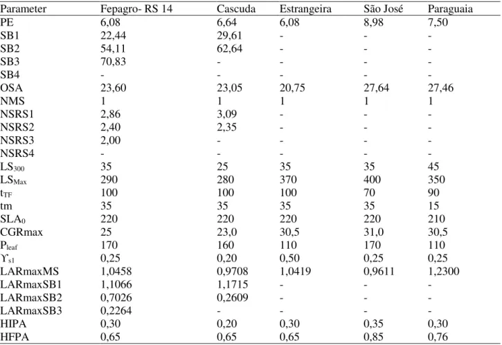
Table 2 contains the Simanihot genetic parameters calibrated for each cultivar. Each cultivar has a development period until emergence, OSA, and BS1, BS2, BS3, BS4. From BS1 to BS4 are represented the morphological differences among cultivars, some of them can branch up to three times (Fepagro-RS 14), while others have no branching during the growing season (Estrangeira, São José, and Paraguaia). The parameters influencing leaf size (LS300, LSMax, tTF, tm) also vary with cultivar. For cultivars branching more than once (Fepagro - RS 14, Cascuda), LSMax is lower than the calibrated for cultivars without branching (Estrangeira, São José, and Paraguaia). Each cultivar has its own LARmax, which means that each genotype has a different leaf appearance rate (Table 2).
TABLE 2. Genetic parameters in the Simanihot model calibrated for the cassava cultivars Fepagro-RS 14, Cascuda, Estrangeira, São José and Paraguaia.
Parameter Fepagro- RS 14 Cascuda Estrangeira São José Paraguaia
PE SB1 SB2 SB3 SB4 OSA NMS NSRS1 NSRS2 NSRS3 NSRS4 LS300
LSMax
tTF
tm SLA0
CGRmax Pleaf
ϒs1
LARmaxMS LARmaxSB1 LARmaxSB2 LARmaxSB3 HIPA
HFPA
6,08 22,44 54,11 70,83 - 23,60 1 2,86 2,40 2,00 - 35 290 100 35 220 25 170 0,25 1,0458 1,1066 0,7026 0,2264 0,30 0,65
6,64 29,61 62,64 - - 23,05 1 3,09 2,35 - - 25 280 100 35 220 23,0 160 0,20 0,9708 1,1715 0,2609 - 0,20 0,65
6,08 - - - - 20,75 1 - - - - 35 370 100 35 220 30,5 110 0,50 1,0419 - - - 0,30 0,65
8,98 - - - - 27,64 1 - - - - 35 400 70 35 220 31,0 170 0,25 0,9611 - - - 0,35 0,85
7,50 -
- - - 27,46 1 - - - - 45 350 90 15 210 30,5 110 0,25 1,2300 - - - 0,30 0,76
* PE (Developmental time from planting to emergence, Dd); SB1, SB2, SB3, SB4 (Developmental time from emergence and the first simpodial branching (SB1), second simpodial branching (SB2), third simpodial branching (SB3), fourth simpodial branching (SB4) Dd); OSA (Developmental time from emergence and onset of starch accumulation, Dd); NMS (Number of the main stem); NSRS1 (Number of stems in the BS1); NSRS2 (Number of stems in the BS2); NSRS3 (Number of stems in the BS3); NSRS4 (Number of stems in the BS4); LS300 (Leaf size at 300 days after emergence (DAE), cm²); LSmax (Maximum leaf size, cm²); tTF
(Date at which max leaf size occurs DAE); tm (Form coefficient in the leaf size equation); SLA0 (Specific leaf área for the one
cultivar at a temperature of the 24ºC and without water stress, cm²/g); CGRmax (Maximum crop growth rate, g/m² dia); Pleaf (Maximum leaf age, dias); ϒs1 (Coefficient of senescence sensitivity to shading when Tmin> 5,0 ºC); LARmaxMS, LARmaxSB1,
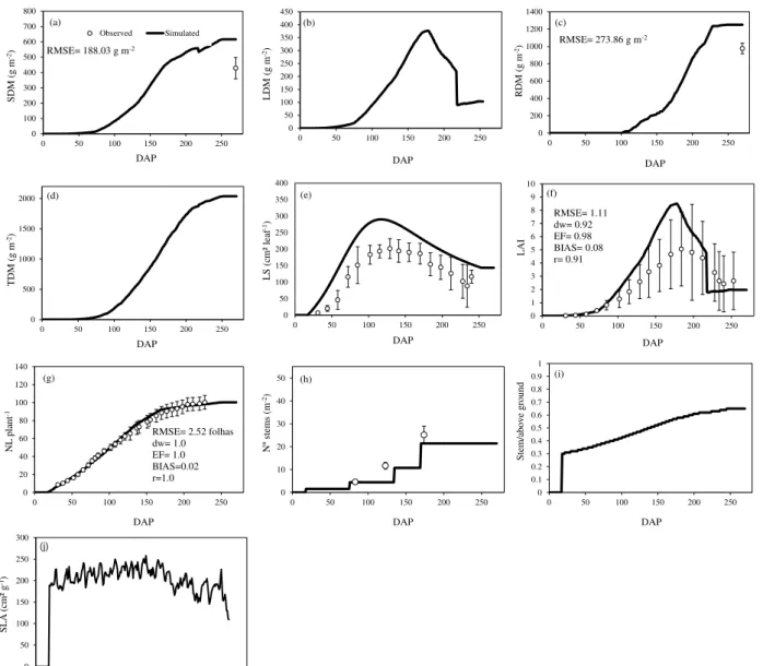
When running the model with independent data (Table 1), no differences were observed regarding growth, development, and yield variables simulated both with the water balance activated or not, indicating that soil moisture was not a limiting factor for the crop during growing season and in all experiments. Figures 1 and 5 show Simanihot simulation for each cultivar in one growing season. The other simulations with statistics are shown in Table 3.
For Fepagro-RS 14 (Figure 1), the RMSE of stem dry mass (SDM) values was 188.03 g m-2, corresponding to 1.88 ton ha-1; RMSE for root dry mass (RDM) was 273.86 g m-2, i.e. 2.74 ton ha-1. LAI had an RMSE of 1.11; while dw, EF, and r were above 0.9, and BIAS index reached 0.08; therefore, the observed values were overestimated. As a forage cultivar, it is compound of large-sized plants with great shoot-yielding variability, reflecting in high standard deviation LAIs. Thus, in this process, the observed values had a great variability what brought about LAI overestimation. Leaf number presented an RMSE of 2.52 leaves, with dw, EF, and r at a maximum value (1.00), and BIAS index of 0.02, indicating good performance of the Simanihot model. The number of stems simulated by the model, in general, followed the same trend of the observed ones (Figure 1h).
TABLE 3. Statistics of the evaluation of the performance of the Simanihot model for cassava cultivars in different growing seasons in Santa Maria and Vera Cruz, RS.
Site/Cultivar/
growing season Statistic
Stem * (g m-2)
Leaves* (g m-2)
Roots* (g m-2)
Total* (g m-2)
LAI* NL*
(leaves pl-1) Santa Maria
2014/2015 RMSE dw EF BIAS r
34.07 0.98 0.99 0.14 0.98
49.52 0.72 0.64 0.82 0.82
246.30 0.88 0.86 0.64 1.00
316.47 0.90 0.90 0.50 0.99
0.93 0.78 0.82 0.42 0.71
- - - - -
* Stem (stem dry matter; Leaves (leaves dry matter); Roots (roots dry matter), Total (total dry matter); LAI (leaf area index); NL (number of leaves per plant).
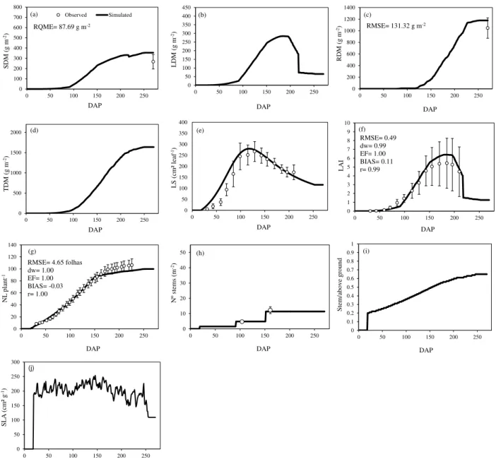
The simulation for Cascuda, in 2011-2012, resulted in SDM values slightly smaller (Figure 2a) if compared to those simulated with an RMSE of 87.69 g m-2, and RDM of 131.32 g m-2 (Figure 2c), in which the simulated value was within the standard deviation of the observed values. LAI (Figure 2f) presented an RMSE of 0.49, EF of 1.00, dw, and r of 0.99, and BIAS index of 0.11, with simulated values overestimating the observed values. The number of leaves (NL) (Figure 2g) had an RMSE of 4.65 leaves, with dw, EF, and r at its maximum (1.00), and BIAS index of -0.03. It was because at the end of the growing season the simulated values were slightly below those observed ones.
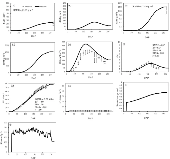
For Estrangeira, in the 2011-2012 growing season, SDM (Figure 3a) showed good results by Simanihot simulation, with an RMSE of 23.09 g m-2; and RDM (Figure 3c) was of 172.56 g m-2, with simulated values above that observed but within the upper standard deviation. LAI (Figure 3f) presented an RMSE of 0.47; EF, dw, and r were near or above 0.9 while BIAS index was of 0.05, with simulated values slightly overestimating the observed ones. NL (Figure 3g) RMSE was 3.27 leaves; dw, EF, and r reached the maximum (1.00), and BIAS index was -0.01 (the closer to zero the better the model).
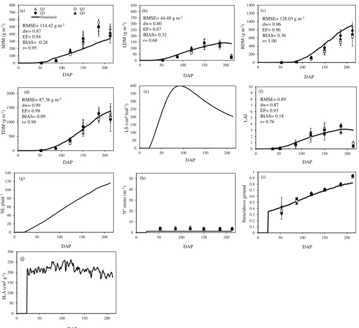
In Vera Cruz, the simulations of São José cultivar (Figure 4) for SDM, LDM, and RDM followed the field trends, with RMSEs of 114.42 g m², 44.48 g m-², and 128.03 g m-² respectively. Likewise, LAI followed the same field trends, with an RMSE of 0.89. Still, there was a marked decrease in LDM and LAI observed values in the last collection (Figure 4b, 4f), what might have been due to an early leaf senescence caused by fungal diseases, which is not been considered in the model.
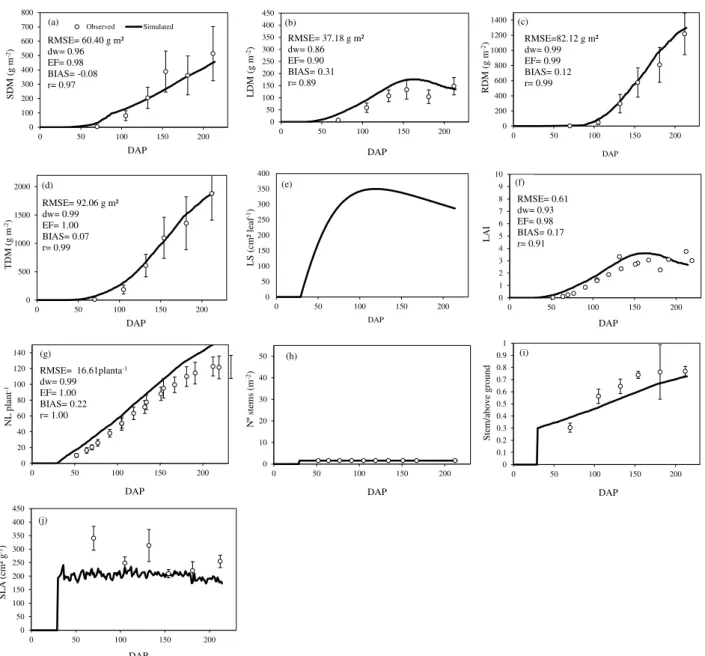
For Paraguaia cultivar, in 2014-2015 (Figure 5), RMSE for SDM, LDM, RDM, and TDM were 60.40, 37.18, 82.12, and 92.06 g m-2, respectively, with a slight LDM overestimation (BIAS = 0.31). LAI reached an RMSE of 0.61, with simulated values within the standard deviation of the observed values. Yet NL had a BIAS index of 0.22, indicating simulation overestimates, with an RMSE of 16.61 leaves plant-1.
Figure 6 (a) and 6 (c) show both the observed and simulated mean values of soil moisture
content by Ritchie’s and Thornthwaite & Mather’s models, during 2014-2015 in Santa Maria
whereas Figure 6 (b) e 6 (d) present the observed and simulated values in Vera Cruz. For Santa Maria, comparisons of observed and simulated values by the mentioned models from the beginning
of the crop cycle has RMSEs of 0.019 cm³/cm³ for Ritchie’s and of 0.023 cm³/cm³ for Thornthwaite
& Mather’s; while for Vera Cruz, these values were 0.033 cm³/cm³ for Ritchie model and 0.028
cm³/cm³ for Thornthwaite & Mather model. Simulated soil moisture had more variations along crop cycle when simulated with the Thornthwaite & Mather model. For this model, soil water contents decreased faster than did those simulated by the Ritchie model, as well as those observed ones. As soil water storage (SWS) depends on its availability (AWC), daily values of rainfall, maximum crop evapotranspiration (ETc), and current water content make up the SWS converted to a volume basis (divided by depth - ze), and added to the AWC lower limit (at permanent wilting point). Thus, lower rainfall values and high ETc demands can lead to a decreased SWS and, consequently, smaller water contents in the soil. As a result, the values simulated by the Thornthwaite & Mather model show greater variability along the crop developmental cycle.
however, providing better responses from the 100 DAP (days after planting). Differently, the Thornthwaite & Mather's model could well represent the mean soil water content in this period. Overall, both models deliver good results for water content in the soil, albeit with advantages and limitations. Thus, the choice depends on the number of available soil variables and on how many layers will be assessed, either a single layer (Thornthwaite & Mather's model) or all layers explored by the roots throughout the crop developmental cycle (Ritchie's model).
Our results show that Simanihot can be used in numerical studies on cassava crop grown in Rio Grande do Sul. However, its use in other areas of Brazil still requires testing. Nevertheless, for being based on processes derived from the GUMCAS model (MATTHEWS & HUNT, 1994), which is well known for cassava in the DSSAT platform, Simanihot has great potential of being used outside the environment of calibration.
0 50 100 150 200 250 300 350 400
0 50 100 150 200 250
L
S
(c
m
² lea
f
-1)
DAP (e)
0 500 1000 1500 2000
0 50 100 150 200 250
TD
M (g
m
-2)
DAP (d)
0 20 40 60 80 100 120 140
0 50 100 150 200 250
NL
plant
-1
DAP (g)
RMSE= 2.52 folhas dw= 1.0 EF= 1.0 BIAS=0.02 r=1.0
0 1 2 3 4 5 6 7 8 9 10
0 50 100 150 200 250
L
AI
DAP (f)
RMSE= 1.11 dw= 0.92 EF= 0.98 BIAS= 0.08 r= 0.91
0 50 100 150 200 250 300 350 400 450
0 50 100 150 200 250
L
DM
(g
m
-2)
DAP (b)
0 200 400 600 800 1000 1200 1400
0 50 100 150 200 250
R
DM
(g
m
-2)
DAP (c)
RMSE= 273.86 g m-2
0 0.1 0.2 0.3 0.4 0.5 0.6 0.7 0.8 0.9 1
0 50 100 150 200 250
S
tem/above
g
round
DAP (i)
0 100 200 300 400 500 600 700 800
0 50 100 150 200 250
S
DM (
g
m
-2)
DAP
Observed Simulated
(a)
RMSE= 188.03 g m-2
0 10 20 30 40 50
0 50 100 150 200 250
Nº ste
ms (m
-2)
DAP (h)
0 50 100 150 200 250 300
0 50 100 150 200 250
S
L
A
(c
m²
g
-1)
DAP
(j)
0 50 100 150 200 250 300 350 400
0 50 100 150 200 250
L
S
(c
m² l
ea
f
-1)
DAP (e)
0 500 1000 1500 2000
0 50 100 150 200 250
TD
M (g
m
-2)
DAP (d)
0 20 40 60 80 100 120 140
0 50 100 150 200 250
NL
plant
-1
DAP (g)
RMSE= 4.65 folhas dw= 1.00 EF= 1.00 BIAS= -0.03 r= 1.00
0 1 2 3 4 5 6 7 8 9 10
0 50 100 150 200 250
L
AI
DAP (f)
RMSE= 0.49 dw= 0.99 EF= 1.00 BIAS= 0.11 r= 0.99
0 50 100 150 200 250 300 350 400 450
0 50 100 150 200 250
L
DM
(g
m
-2)
DAP (b)
0 200 400 600 800 1000 1200 1400
0 50 100 150 200 250
R
DM
(g
m
-2)
DAP (c)
RMSE= 131.32 g m-2
0 0.1 0.2 0.3 0.4 0.5 0.6 0.7 0.8 0.9 1
0 50 100 150 200 250
S
tem/above
g
round
DAP (i)
0 100 200 300 400 500 600 700 800
0 50 100 150 200 250
S
DM (
g
m
-2)
DAP
Observed Simulated
(a)
RQME= 87.69 g m-2
0 10 20 30 40 50
0 50 100 150 200 250
Nº ste
ms (m
-2)
DAP (h)
0 50 100 150 200 250 300
0 50 100 150 200 250
S
L
A
(c
m²
g
-1)
DAP
(j)
0 50 100 150 200 250 300 350 400
0 50 100 150 200 250
L
S
(c
m² l
ea
f
-1)
DAP
(e)
0 500 1000 1500 2000
0 50 100 150 200 250
TD
M
(g
m
-2)
DAP
(d)
0 20 40 60 80 100 120 140
0 50 100 150 200 250
NL
plant
-1
DAP
(g)
RQME = 3.27 folhas dw= 1.00 EF= 1.00 BIAS= -0.01 r= 1.00
0 1 2 3 4 5 6 7 8 9 10
0 50 100 150 200 250
L
AI
DAP
(f) RMSE = 0.47
dw= 0.94 EF= 0.98 BIAS= 0.05 r= 0.89
0 50 100 150 200 250 300 350 400 450
0 50 100 150 200 250
L
DM
(g
m
-2)
DAP (b)
0 200 400 600 800 1000 1200 1400
0 50 100 150 200 250
R
DM
(g
m
-2)
DAP
(c) RMSE= 172.56 g m-2
0 0.1 0.2 0.3 0.4 0.5 0.6 0.7 0.8 0.9 1
0 50 100 150 200 250
S
tem/above
g
round
DAP (i)
0 100 200 300 400 500 600 700 800
0 50 100 150 200 250
S
DM (
g
m
-2)
DAP
Observed Simulated
(a)
RMSE = 23.09 g m-2
0 10 20 30 40 50
0 50 100 150 200 250
Nº ste
ms (m
-2)
DAP (h)
0 50 100 150 200 250 300
0 50 100 150 200 250
S
L
A
(c
m²
g
-1)
DAP
(j)
0 50 100 150 200 250 300 350 400
0 50 100 150 200
L
S
(c
m² l
ea
f
-1)
DAP (e)
0 500 1000 1500 2000
0 50 100 150 200
TD
M
(g
m
-2)
DAP (d)
RMSE= 87.36 g m-2
dw= 0.99 EF= 0.99 BIAS= 0.09 r= 0.99
0 20 40 60 80 100 120 140
0 50 100 150 200
NL
plant
-1
DAP (g)
0 1 2 3 4 5 6 7 8 9 10
0 50 100 150 200
L
AI
DAP (f)
RMSE= 0.89 dw= 0.87 EF= 0.93 BIAS= 0.18 r= 0.76
0 50 100 150 200 250 300 350 400 450
0 50 100 150 200
L
DM
(g
m
-2)
DAP (b)
RMSE= 44.48 g m-2
dw= 0.80 EF= 0.87 BIAS= 0.32 r= 0.68
0 200 400 600 800 1000 1200 1400
0 50 100 150 200
R
DM
(g
m
-2)
DAP (c)
RMSE= 128.03 g m-2
dw= 0.96 EF= 0.96 BIAS= 0.36 r= 1.00
0 0.1 0.2 0.3 0.4 0.5 0.6 0.7 0.8 0.9 1
0 50 100 150 200
S
tem/above
g
round
DAP (i)
0 100 200 300 400 500 600 700 800
0 50 100 150 200
S
DM (
g
m
-2)
DAP
Q1 Q2
Q3 Q4
Simulated
(a)
RMSE= 114.42 g m-2
dw= 0.87 EF= 0.94 BIAS= -0.28 r= 0.95
0 10 20 30 40 50
0 50 100 150 200
Nº ste
ms (m
-2)
DAP (h)
0 50 100 150 200 250 300
0 50 100 150 200
S
L
A
(c
m²
g
-1)
DAP
(j)
0 50 100 150 200 250 300 350 400
0 50 100 150 200
L
S
(c
m² l
ea
f
-1)
DAP
(e)
0 500 1000 1500 2000
0 50 100 150 200
TD
M
(g
m
-2)
DAP (d)
RMSE= 92.06 g m² dw= 0.99 EF= 1.00 BIAS= 0.07 r= 0.99
0 20 40 60 80 100 120 140
0 50 100 150 200
NL
plant
-1
DAP (g)
RMSE= 16.61planta-1
dw= 0.99 EF= 1.00 BIAS= 0.22 r= 1.00
0 1 2 3 4 5 6 7 8 9 10
0 50 100 150 200
L
AI
DAP (f)
RMSE= 0.61 dw= 0.93 EF= 0.98 BIAS= 0.17 r= 0.91
0 50 100 150 200 250 300 350 400 450
0 50 100 150 200
L
D
M
(g
m
-2)
DAP (b)
RMSE= 37.18 g m² dw= 0.86 EF= 0.90 BIAS= 0.31 r= 0.89
0 200 400 600 800 1000 1200 1400
0 50 100 150 200
R
DM (
g
m
-2)
DAP
(c)
0 0.1 0.2 0.3 0.4 0.5 0.6 0.7 0.8 0.9 1
0 50 100 150 200
S
tem/above
g
round
DAP (i)
0 100 200 300 400 500 600 700 800
0 50 100 150 200
S
DM (
g
m
-2)
DAP
Observed Simulated
(a)
RMSE= 60.40 g m² dw= 0.96 EF= 0.98 BIAS= -0.08 r= 0.97
0 10 20 30 40 50
0 50 100 150 200
Nº ste
ms (m
-2)
DAP (h)
0 50 100 150 200 250 300 350 400 450
0 50 100 150 200
S
L
A
(c
m²
g
-1)
DAP (j)
RMSE=82.12 g m² dw= 0.99 EF= 0.99 BIAS= 0.12 r= 0.99
0 20 40 60 80 100 120
0.15 0.2 0.25 0.3 0.35 0.4 0.45
0 50 100 150 200
R
ainfa
ll
(mm)
S
oil
wa
ter
c
ontent
(c
m³/
cm³)
DAP Rainfall
SW Obs SW Ritchie
(a) RMSE= 0.019 cm³/cm³
dw = 0.71 EF= 0.99 BIAS= 0.04 r= 0.66
0 20 40 60 80 100 120
0.15 0.2 0.25 0.3 0.35 0.4 0.45
0 50 100 150 200
R
ain
fall
(m
m
)
S
oil
wa
ter
c
ontent
(c
m³/
cm³)
DAP Rainfall
SW Obs SW TM
(c) RMSE= 0.023 cm³/cm³
dw = 0.73 EF= 0.99 BIAS= -0.01 r= 0.69
0 10 20 30 40 50 60 70 80
0 0.05 0.1 0.15 0.2 0.25 0.3
0 50 100 150 200
R
ainfa
ll
(mm)
S
oil
wa
ter
c
ontent
(c
m³/
cm³)
DAP
(b) RMSE= 0.033 cm³/cm³ dw= 0.71 EF= 0.99 BIAS= 0.14 r= 0.65
0 10 20 30 40 50 60 70 80
0 0.05 0.1 0.15 0.2 0.25 0.3
0 50 100 150 200
R
ainfa
ll
(mm)
S
oil
wa
ter
c
ontent
(c
m³/
cm³)
DAP
(d) RMSE= 0.028 cm³/cm³ dw= 0.83 EF= 1.0 BIAS= -0.01 r= 0.73
FIGURE 6. Soil water content observed (open circles) and simulated with the Ritchie model (solid line) and with the Thornthwaite and Mather model (dashed line) in the experiment with cassava in Santa Maria (a,c) and in a commercial farm in Vera Cruz (b,d), and rainfall during the crop growing season (from planting to harvest) as a function of Days After Planting (DAP) during the 2014-2015 growing season. RMSE=root mean square error, dw=index of agreement, EF-model efficiency, BIAS=bias index, r=correlation coefficient.
CONCLUSIONS
Simanihot model has good performance in simulations of cassava growth, development, and yield. The model runs at a one-day time step, being calibrated for five cassava cultivars (Fepagro - RS 14, Estrangeira, Cascuda, São José, and Paraguaia), which have different branching habits and usages (forage, table, and industry ). Also, this model has a graphical interface that allows users to select one of two soil water balance models. Both evaluated models of water balance well represent the actual water content in the soil. Finally, the soil model choice will depend on the number of known soil variables and the desired detailing.
REFERENCES
DOURADO-NETO, D. et al. Balance hídrico ciclico y secuencial : estimación de almacenamiento de agua en el suelo. Scientia Agricola, Piracicaba, v. 56, n. 3, p. 537-546, 1999. Disponível em: <http://www.scielo.br/scielo.php?script=sci_arttext&pid=S0103-90161999000300005>. Acesso em: 11 fev. 2016.
GABRIEL, L. F.; STRECK, N. A.; ROBERTI, D. R.; CHIELLE, Z. G.; UHLMANN, L. O.; SILVA, M. R. da.; SILVA, S. D. da. Simulating cassava growth and yield under potential conditions in Southern Brazil. Agronomy Journal, Madison, v. 106, n. 4, p. 1119-1137, 2014. Disponível em:
<https://dl.sciencesocieties.org/publications/aj/abstracts/106/4/1119?access=0&view=pdf>. Acesso em: 11 fev. 2016.
KIM, S.; YANG, Y.; TIMLIN, D.J.; FLEISHER, D.H.; DATHE, A.; REDDY, V.R.; STAVER, K. Modeling temperature responses of leaf growth, development, and biomass in maize with
MAIZSIM. Agronomy Journal, Madison, v. 104, p. 1523-1537, 2012. Disponível em: <
LAGO, I.; STRECK, N.A.; BISOGNIN, D.A.; SOUZA, A.T.de.; SILVA, M.R.da. Transpiração e crescimento foliar de plantas de mandioca em resposta ao deficit hídrico no solo. Pesquisa
Agropecuária Brasileira, Brasília, DF, v. 46, p. 1415-1423, 2011. Disponível em: < www.scielo.br/pdf/pab/v46n11/v46n11a01.pdf>. Acesso em: 11 fev. 2016.
MATTHEWS, R.B.; HUNT, L.A. GUMCAS: A model describing the growth of cassava (Manihot esculenta L. Crantz). Field Crops Research, Amsterdam, v. 39, p. 69–84, 1994. Disponível em: < http://www.sciencedirect.com/science/article/pii/037842909490054X>. Acesso em: 11 fev. 2016.
NASSIF, D.S.P.; MARIN, F.R.; FILHO, W.J.P.; RESENDE, R.S.; PELLEGRINO, G.Q. Parametrização e avaliação do modelo DSSAT/Canegro para variedades brasileiras de cana-de-açúcar. Pesquisa Agropecuária Brasileira, Brasília, DF, v. 47, p. 311-318, 2012. Disponível em: <http://www.scielo.br/scielo.php?script=sci_arttext&pid=S0100-204X2012000300001>. Acesso em: 11 fev. 2016.
PINHEIRO, D.G.; STRECK, N.A.; RICHTER, G.L.; LANGNER, J.A.; WINCK, J.E.M.;
UHLMANN, L.O.; ZANON, A.J. Limite crítico de água no solo para transpiração e crescimento foliar em mandioca em dois períodos com deficiência hídrica. Revista Brasileira de Ciência do
Solo, Viçosa, MG, v. 39, p. 1740-1749, 2014. DOI: 10.1590/S0100-06832014000600009
SAMBORANHA, F.K.; STRECK, N.A.; UHLMANN, L.O.; GABRIEL, L.F. Modelagem
matemática do desenvolvimento foliar em mandioca. Revista Ciência Agronômica, Fortaleza, v. 44, p. 815-824, 2013. Disponível em:
<http://ccarevista.ufc.br/seer/index.php/ccarevista/article/view/2326>. Acesso em: 11 fev. 2016.
SINGH, S.S.; BOOTE, K.J.; ANGADI, S.V.; GROVER, K.; BEGNA, S.; AULD, D. Adapting the CROPGRO Model to Simulate Growth and Yield of Spring Safflower in Semiarid Conditions.
Agronomy Journal, Madison, v. 108, p. 64-72, 2016. Disponível em:
<https://dl.sciencesocieties.org/publications/aj/tocs/108/1>. Acesso em: 11 fev. 2016.