Quantitative assessment of Southern Hemisphere ozone in chemistry-climate model simulations

(1)

www.atmos-chem-phys.net/10/1385/2010/ © Author(s) 2010. This work is distributed under the Creative Commons Attribution 3.0 License.

Chemistry

and Physics

Quantitative assessment of Southern Hemisphere ozone in

chemistry-climate model simulations

A. Yu. Karpechko1,*, N. P. Gillett2, B. Hassler3,4,5, K. H. Rosenlof4, and E. Rozanov6,7 1_{Climatic Research Unit, School of Environmental Sciences, University of East Anglia, UK} 2_{Canadian Centre for Climate Modelling and Analysis, Environment Canada, Canada} 3_{National Institute of Water and Atmospheric Research, Lauder, New Zealand} 4_{NOAA, Earth System Research Laboratory, Boulder, USA}

5_{Cooperative Institute for Research in Environmental Sciences, University of Colorado, Boulder, USA} 6_{Institute for Atmospheric and Climate Science, ETH Z¨urich, Switzerland}

7_{Physical-Meteorological Observatory/World Radiation Center, Davos, Switzerland} *_{now at: Finnish Meteorological Institute, Arctic Research, Helsinki, Finland}

Received: 6 July 2009 – Published in Atmos. Chem. Phys. Discuss.: 17 September 2009 Revised: 15 January 2010 – Accepted: 25 January 2010 – Published: 8 February 2010

Abstract. Stratospheric ozone recovery in the Southern

Hemisphere is expected to drive pronounced trends in atmo-spheric temperature and circulation from the stratosphere to the troposphere in the 21st century; therefore ozone changes need to be accounted for in future climate simulations. Many climate models do not have interactive ozone chemistry and rely on prescribed ozone fields, which may be obtained from coupled chemistry-climate model (CCM) simulations. How-ever CCMs vary widely in their predictions of ozone evo-lution, complicating the selection of ozone boundary condi-tions for future climate simulacondi-tions. In order to assess which models might be expected to better simulate future ozone evolution, and thus provide more realistic ozone boundary conditions, we assess the ability of twelve CCMs to simulate observed ozone climatology and trends and rank the models according to their errors averaged across the individual diag-nostics chosen. According to our analysis no one model per-forms better than the others in all the diagnostics; however, combining errors in individual diagnostics into one metric of model performance allows us to objectively rank the mod-els. The multi-model average shows better overall agreement with the observations than any individual model. Based on this analysis we conclude that the multi-model average ozone projection presents the best estimate of future ozone evolu-tion and recommend it for use as a boundary condievolu-tion in future climate simulations. Our results also demonstrate a sensitivity of the analysis to the choice of reference data set

Correspondence to:A. Yu. Karpechko

(alexey.karpechko@fmi.fi)

for vertical ozone distribution over the Antarctic, highlight-ing the constraints that large observational uncertainty im-poses on such model verification.

1 Introduction

In the last two decades of the 20th century stratospheric ozone, which accounts for about 90% of the total ozone, has declined significantly as a result of chemical destruction by anthropogenic halogen-containing compounds (WMO, 2007). In the Southern Hemisphere (SH) where ozone deple-tion is particularly severe in high-latitudes in spring, ozone changes have led to cooling of the lower stratosphere and an increase in the lifetime of the Antarctic polar vortex (e.g., Randel and Wu, 1999; Zhou et al., 2000). These changes have further led to intensification of the tropospheric circum-polar circulation (Thompson and Solomon, 2002; Gillett and Thompson, 2003). Among other impacts, the intensification of the tropospheric circulation has contributed to significant decrease of rainfalls in southwest Australia (Cai et al., 2005) and to dramatic warming of the Antarctic Peninsula (Mar-shall et al., 2006).

(2)

change to the tropospheric circulation is unclear (Miller et al., 2006; Perlwitz et al., 2008; Son et al., 2008, 2009). This implies that details of the ozone recovery need to be pre-dicted well in order to reliably simulate future SH climate.

Presently, full representation of stratospheric chemistry in climate models is quite expensive and the majority of coupled atmosphere-ocean climate models use prescribed ozone fields. Models that were used for the Intergovern-mental Panel of Climate Change Forth Assessment Report (IPCC AR4) used either a simplified ozone recovery sce-nario or even assumed constant ozone (i.e. annual cycle not varying from year to year) throughout the 21st century (Miller et al., 2006). More physically sound future ozone scenarios are provided by coupled Chemistry-Climate Mod-els (CCMs). These modMod-els account for interactions between stratospheric ozone chemistry and atmospheric physics and dynamics which may change due to projected greenhouse gases (GHGs) increases. However ozone projections by these models differ from model to model (Eyring et al., 2007) raising the question of which ozone scenario is more reliable. Information on model performance in simulating present climate may be used to decide which model’s projection is more reliable (Reichler and Kim, 2008; Gleckler et al., 2008). However models are tuned to represent the present climate and the best tuned model may not simulate future cli-mate more correctly. Yet, without a better alternative, model ranking based on their ability to simulate present climate and observed trends looks like a reasonable approach and is widely employed (e.g. Connolley and Bracegirdle, 2007; Bracegirdle et al., 2008).

Eyring et al. (2006) assessed different aspects of perfor-mance of several CCMs including their ozone simulation skill; however they did not derive any quantitative metric of agreement between simulations and observations. Waugh and Eyring (2008) (hereinafter “WE08”) carried out a quan-titative assessment of CCMs’ ability to simulate several key processes relevant to stratospheric ozone since they argued that a process-oriented evaluation might be a better predictor of a models’ ability to make reliable ozone projections; be-cause of that they did not assess models’ skill at simulating ozone itself. Nevertheless, it is important to assess models’ ability to simulate ozone climatology and trends; our study may be considered a complimentary to that of WE08. It is also of interest to look at how models skill in simulating ozone-related processes correlates with their skill in simu-lating ozone itself. The goal of this study is to provide cli-mate modellers with a guideline for choice of future ozone scenario for simulations with prescribed ozone fields. To achieve this we perform a quantitative assessment of CCM skills in simulating observed ozone climatology and ozone trends with a focus on the SH, where the largest impacts of ozone recovery on the climate are expected. As a refer-ence, we employ several available up-to-date observational data sets, which allow us to evaluate uncertainties associated with the observations.

Table 1.CCMs used in this study.

Model name Reference

CCSRNIES Akiyoshi et al. (2004)

CMAM Fomichev et al. (2007)

E39C Dameris et al. (2005)

GEOSCCM Pawson et al. (2008)

LMDZrepro Jourdain et al. (2008)

MAECHAM4CHEM Steil et al. (2003)

MRI Shibata and Deushi (2005)

SOCOL Egorova et al. (2005)

ULAQ Pitari et al. (2002)

UMETRAC Austin (2002)

UMSLIMCAT Tian and Chipperfield (2005)

WACCM Garcia et al. (2007)

2 Data

(3)

Observational data sets used for model performance vali-dation include total ozone and ozone profiles data sets from several sources. The merged satellite total ozone data set (TOMS/SBUV) is based on individual Total Ozone Map-ping Spectrometer (TOMS) and Solar Backscatter Ultravi-olet 2 (SBUV/2) data sets (Stolarski and Frith, 2006). An-other total ozone data set used in this study is that compiled by Karen Rosenlof from satellite (SME, SAGE-II, MLS, HALOE and TOMS/SBUV) and standard ozone climatology data (Dall’Amico et al., 2010). The Rosenlof data set also provides ozone profiles. Two other ozone profile data sets used here are those described in papers by Randel and Wu (2007) and Hassler et al. (2009). The former (Randel data set) is based on a regression model fitted to SAGE 1 and 2 and ozonesonde profiles combined with a seasonally varying ozone climatology. Over the Antarctic region, which is of in-terest here, the model utilises only data from Syowa station located at 69◦_{S and may not adequately represent the ozone}

field further south. Implications of this will be discussed be-low. The Randel data set is provided on the height levels. These was converted to pressure levels applying the equation 1013.25∗_exp(₋_z_{/7), where}_z_{is height expressed in}

kilome-tres. The latter data set (Hassler data set) is based on satellite (SAGE 1 and 2, POAM 2 and 3, HALOE) and ozonesonde profiles. Due to the lack of the observations, the Rosenlof and the Hassler data sets also apply different techniques to fill in the gaps, which will be discussed in more detail below.

3 Method

To assess model performance we calculate a metric similar to that used by Reichler and Kim (2008) and Gleckler et al. (2008). First we calculate normalized root mean square (RMS) differencesej klbetween thej-th model andk-th

ref-erence observations for thel-th diagnostic

e_{j kl}2 ₌ 1 W

X

i

X

m

(wim(ximj l−yimkl)2/σimkl2 ), (1)

whereximj l is the simulated variable and yimkl is the

ob-served variable at monthmand grid pointi,wimis the weight

assigned to each data point,W=Pw, is a sum of individ-ual weights andσimklis a measure of the uncertainty in the

observed variableyimkl. In the following the valueej kl will

be referred to as model error inl-th diagnostic with respect tok-th reference observations. Calculations of the weights and the observation uncertainty are described below in this section.

Following Reichler and Kim (2008) we scale the errors in all diagnostics by the average error across the individ-ual models to ensure that different diagnostics receive

sim-ilar weights when calculating the combined metric of model performance

e′2

j kl=

e_{j kl}2

1

J

P

j

e_{j kl}2 , (2)

where J is the number of models. Model errors are cal-culated with respect to several available observation-based data sets in order to reduce possible influence of biases in the observation-based data sets. However, the observation data sets are not completely independent since they share some of the same input data and therefore may suffer from similar biases. We next average the model errors with respect to all available reference data sets for each diagnostic

e′2

j l=

1 K

X

k

e′2

j kl, (3)

where K is the number of reference data sets. Finally, a model performance index (I) is calculated as an average across errors in all individual diagnostics

I_j2₌1 L

X

l

e′2

j l, (4)

whereLis the number of diagnostics. A lower value ofI indicates better overall agreement with the observations and is interpreted as a better model performance.

(4)

Table 2.Diagnostics used in this study.

Diagnostic Diagnostic description

Global total ozone climatology Total ozone climatology in 1980–1984, zonal mean monthly mean values, domain: 90◦_S–90◦_{N, resolution: 5}◦

SH total ozone trend Total ozone linear trend between 1980–1999, zonal mean monthly mean values,

domain: 90◦_S–0◦_{N, resolution: 5}◦

Polar SH vertical ozone distribution climatology Ozone partial pressure profile climatology in 1980-1984, monthly mean values av-eraged over 90◦_S–60◦_{S, levels: 500, 400, 300, 250, 200, 150, 130, 115, 100, 90,}

80, 70, 50, 30, 20, 15, 10 hPa

Polar SH vertical ozone distribution trend Ozone partial pressure profile linear trend between 1980–1999, monthly mean val-ues averaged over 90◦_S–60◦_{S, levels: 500, 400, 300, 250, 200, 150, 130, 115, 100,}

90, 80, 70, 50, 30, 20, 15, 10 hPa

TOMS/SBUV

J F M A M J J A S O N D J -50

0 50

Latitude

Rosenlof

0 50

CCSRNIES

0 50

CMAM

0 50

E39C

0 50

Latitude

GEOSCCM

0 50

LMDZrepro

0 50

MAECHAM4CHEM

0 50

MRI

0 50

Latitude

SOCOL

0 50

ULAQ

0 50

UMETRAC

0 50

UMSLIMCAT

0 50

Latitude

WACCM

0 50

MULTI

0 50

175 250 325 400 475

[DU]

(5)

Brewer-Dobson circulation. The latter has experienced a sig-nificant change during the last two decades of the 20th cen-tury (e.g. Hu and Tung, 2002, Karpetchko and Nikulin, 2004) due to reasons which are not completely understood (Hu et al., 2005). This leaves a possibility that natural decadal vari-ability, not related to external forcing, has considerably con-tributed into the NH trends. It is therefore not reasonable to expect that the models simulate the NH trends over 20 years correctly.

The simulation of realistic climate and climate trends de-pends not only on a correct simulation of total column ozone, but also on the vertical distribution of ozone. Therefore two additional diagnostics are considered here: (3) the monthly mean zonal mean vertical ozone distribution climatology over the period 1980–1984 and (4) the monthly mean zonal mean vertical ozone distribution trend over the period 1980– 1999 at several pressure levels (see Table 2 for the list of pressure levels). As discussed in the Introduction the largest influence of stratospheric ozone changes on climate in the 21st century is expected in the SH associated with Antarc-tic ozone hole recovery. Therefore, to put more weight on model skill in simulating ozone over the Antarctic we aver-age vertical ozone distributions only over the SH polar cap (60◦_–90◦_{S) and weight the errors by the annually-average}

ozone profile, i.e. according to their contribution to the total ozone.

Total ozone from all the data sets is linearly interpolated onto a 5◦ _{latitude grid (87.5}◦_{S. . . 87.5}◦_{N). Ozone profiles}

are interpolated linearly in the logarithm of pressure onto the pressure levels specified in Table 2. As a measure of the observational uncertaintyσ, the standard error of the mean is used in the case of the ozone climatology, and the standard error of the slope parameter from a linear regression is used in the case of ozone trends. Measurement errors are only available for the Hassler data set. We calculate measurement errors for our diagnostics using the law of combination of errors:

σ′2

iml=

X

n

( ∂fl ∂yimn

)2σ_imn2 , (5)

whereyimn andσimnare individual observations and errors

at monthmand grid pointiandfl is either the function for

the mean in the case of the climatology, or the function for the slope parameter in the case of the trend. These measure-ment errors are combined with the sampling errors (i.e. with the standard error of the mean or with the standard error of the slope parameter) at each month and grid point by root mean squares and the resultingσ are used for all the three profile data sets.

4 Results

4.1 Total ozone

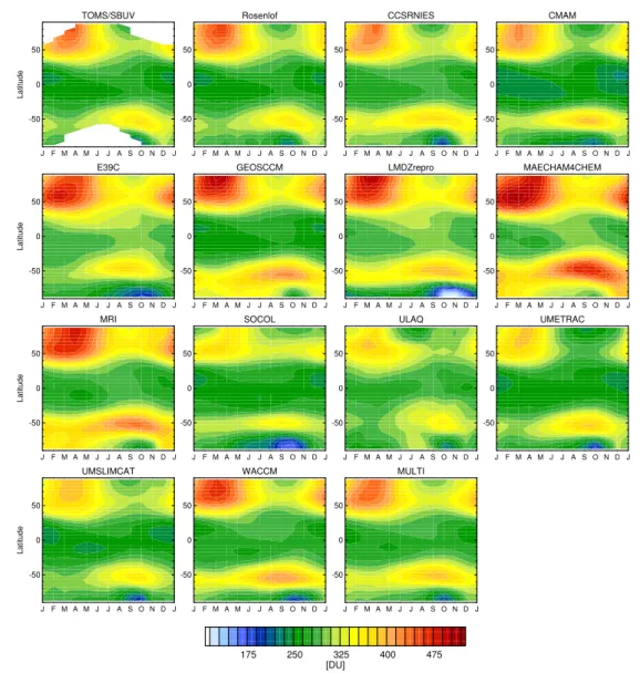
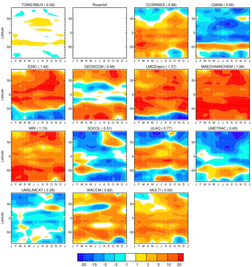
Figure 1 shows 5-year total ozone climatology for the period 1980-1984 from the individual models, MULTI, TOMS/SBUV, and the Rosenlof data set. This picture is sim-ilar to Fig. 14 from Eyring et al. (2006) except that they show 20-year total ozone climatology (1980–1999) and NIWA data set instead of the Rosenlof data set shown here. Also we show an updated MRI simulation. All the models simulate familiar features of the ozone distribution including the win-tertime build-up in both hemispheres, and also the early stage of the Antarctic springtime ozone depletion. Figure 2 shows models and TOMS/SBUV relative errors (xim−yim)/σim

with respect to the Rosenlof data set. Agreement between the two observational data sets is excellent, as might be ex-pected since prior to 1985 the Rosenlof data set employs only data from TOMS and SBUV.

Figures 1–2 show that some models (MAECHAM4-CHEM, MRI) strongly overestimate total ozone globally while others (SOCOL, UMETRAC) strongly underestimate it in the extratropics. Some models (E39C, LMDZrepro) un-derestimate total ozone in SH mid- and high-latitudes while overestimating it elsewhere. In many models the errors typ-ically exceed 3σ, and are therefore very unlikely to be ex-plained by sampling variability associated with the particu-lar 5-yr period chosen for comparison. Eyring et al. (2006) identified the causes of some model errors, like the positive biases in the extratropics in some models which is likely due to the simulated Brewer-Dobson circulation being too strong. However in most cases the causes are not straightforward to identify. MULTI tends to overestimate total ozone, es-pecially in the SH mid-latitudes where several models show strong positive biases. In general there are no consistent bi-ases in total ozone across the models.

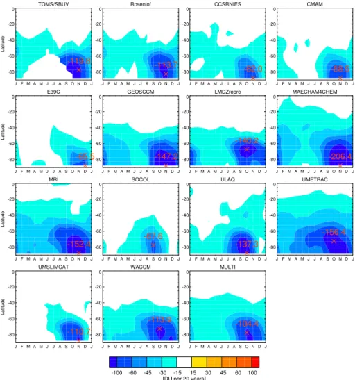
20-year linear trends in total column ozone are shown in Fig. 3. The largest negative trends according to the ob-servations are in the SH high-latitudes in November. All the models simulate a maximum negative trend in the SH high-latitudes but the time varies between September and December. Also the magnitude of the trend differs con-siderably between the models. The smallest simulated trend is only a half of the observed trend (E39C) while the largest trend exceeds the observed trend almost by fac-tor 2 (MAECHAM4CHEM). Eyring et al. (2006) showed that the simulated Antarctic ozone trends are consistent with the trends in Antarctic stratospheric halogen loading. The largest trends in Clyare simulated by UMETRAC while the

smallest trends are simulated by E39C and SOCOL. Accord-ingly, these models simulate too large and too small ozone trends (Eyring et al., 2006). According to WE08 assess-ment UMETRAC has high grade in simulating Antarctic Cly

(6)

TOMS/SBUV ( 0.08)

J F M A M J J A S O N D J

-50 0 50

Latitude

Rosenlof

JF M A M J J A S O N D J

-50 0 50

CCSRNIES ( 0.68)

-50 0 50

CMAM ( 0.65)

-50 0 50

E39C ( 1.42)

-50 0 50

Latitude

GEOSCCM ( 0.68)

-50 0 50

LMDZrepro ( 1.37)

-50 0 50

MAECHAM4CHEM ( 1.94)

-50 0 50

MRI ( 1.15)

-50 0 50

Latitude

SOCOL ( 0.51)

-50 0 50

ULAQ ( 0.77)

-50 0 50

UMETRAC ( 0.60)

-50 0 50

UMSLIMCAT ( 0.28)

-50 0 50

Latitude

WACCM ( 0.62)

-50 0 50

MULTI ( 0.55)

-50 0 50

-20 -10 -5 -3 -1 1 3 5 10 20

σ

Fig. 2. Normalised errors with respect to Rosenlof data set in total ozone climatologies shown in Fig. 1. Numbers next to data set names indicate area-weighted globally averaged errors normalised by the average error across the individual models according to Eq. (2).

Clyvalues are considerably closer to the observed ones than

those used by WE08 but still remain smaller than those in observations and in the majority of CCMVal-1 models (not shown).

Figure 4 shows relative errors with respect to the Rosenlof data set. The TOMS/SBUV biases are small, indicating consistency between TOMS/SBUV and the other satellites (SAGE-II, MLS, HALOE) employed in the Rosenlof data set after 1985. Models that overestimate the magnitude of the trends typically show the largest errors. As a result MULTI trends are biased negative. However the MULTI total error with respect to the Rosenlof data set (and also to TOMS/SBUV) is smaller than in any individual model. MULTI errors are everywhere within 3σ of the observed trends. The CCMVal models almost all show too much ozone depletion in the tropics, but elsewhere biases are not consis-tent in sign amongst the models.

To test the sensitivity of our results to the trend period we calculated the trends for the period 1980–2001 for

observa-tions and for those models for which the data are available. The observed trends for this period are typically smaller than those shown in Fig. 3; however the errors patterns do not change much and our conclusions are unaffected by these changes.

4.2 Vertical ozone distribution

(7)

TOMS/SBUV

JF M A M J J A S O N D J -80

-60 -40 -20 0

Latitude

-119.8

Rosenlof

-60 -40 -20 0

-113.7

CCSRNIES

-60 -40 -20 0

-82.0

CMAM

-60 -40 -20 0

-88.5

E39C

-60 -40 -20 0

Latitude

-65.5

GEOSCCM

-60 -40 -20 0

-147.2

LMDZrepro

-60 -40 -20 0

-140.2

MAECHAM4CHEM

-60 -40 -20 0

-206.4

MRI

-60 -40 -20 0

Latitude

-152.4

SOCOL

-60 -40 -20 0

-67.6

ULAQ

-60 -40 -20 0

-137.3

UMETRAC

-60 -40 -20 0

-156.4

UMSLIMCAT

-60 -40 -20 0

Latitude

-110.7

WACCM

-60 -40 -20 0

-113.9

MULTI

-60 -40 -20 0

-104.4

-100 -60 -45 -30 -15 15 30 45 60 100 [DU per 20 years]

Fig. 3. 20-yr total ozone trends (1980–1999) in observational data sets (TOMS/SBUV, Rosenlof), individual CCMVal models and multi-model average (MULTI). Red numbers indicate minimum trends.

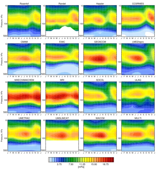
apparent throughout the year. Several other models simu-late too much ozone during the winter build-up period, which may be an indication of either a too strong Brewer-Dobson circulation, or weak isolation of the lower stratospheric polar vortex from mid-latitude ozone-rich air, or both.

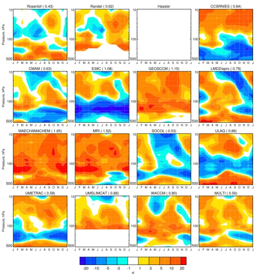
Figure 6 shows model errors in vertical ozone distribution climatology with respect to the Rosenlof data set. The differ-ences between the observational data sets are striking. The Randel data set has typically larger values than the two other data sets especially in spring and summer. This maybe be-cause the Randel data set comprises only data from Syowa station located relatively close to the polar vortex edge (Ran-del and Wu, 2007). The polar vortex edge region is more in-fluenced by mixing with mid-latitude ozone-rich air while air from the vortex interior further south, impacted by chemical ozone depletion, remains more isolated. Reassuringly, both the Randel and the Hassler data set total biases are lower than those of individual models and MULTI, although the differences between the data sets often exceed 3σ. The

dif-ferences between the Rosenlof and the Hassler data sets are largest in the troposphere where no satellite data is avail-able and both data sets rely on a reconstruction to fill in the gaps. In the Rosenlof data set tropospheric ozone is obtained as a difference between total ozone and stratospheric ozone (Dall’Amico et al., 2010) while in the Hassler data set it is calculated it as a regression fit to ozonesonde data, mainly available after 1986 (Hassler et al., 2008), using equiva-lent effective stratospheric chlorine, QBO, solar cycle, El Nino Southern Oscillation, and stratospheric aerosol load-ing resultload-ing from volcanic eruptions (Hassler et al., 2009). The large differences in the stratosphere during winter when satellite coverage of high-latitudes is limited, are also, most probably, related to the differences in the reconstruction tech-niques.

(8)

TOMS/SBUV ( 0.22)

-80 -60 -40 -20 0

Latitude

Rosenlof

-80 -60 -40 -20

0 CCSRNIES ( 0.76)

-80 -60 -40 -20

0 CMAM ( 0.68)

-80 -60 -40 -20 0

E39C ( 0.93)

-80 -60 -40 -20 0

Latitude

GEOSCCM ( 0.64)

-80 -60 -40 -20

0 LMDZrepro ( 0.76)

-80 -60 -40 -20

0 MAECHAM4CHEM ( 1.42)

-80 -60 -40 -20 0

MRI ( 1.18)

-80 -60 -40 -20 0

Latitude

SOCOL ( 1.02)

-80 -60 -40 -20 0

ULAQ ( 1.05)

-80 -60 -40 -20 0

UMETRAC ( 1.57)

-80 -60 -40 -20 0

UMSLIMCAT ( 0.85)

-80 -60 -40 -20 0

Latitude

WACCM ( 0.59)

-80 -60 -40 -20

0 MULTI ( 0.46)

-80 -60 -40 -20 0

-10 -5 -3 -2 -1 1 2 3 5 10

σ

Fig. 4.Normalised errors with respect to the Rosenlof data set in total ozone trends shown in Fig. 3. Numbers next to data set names indicate area-weighted hemisphere-averaged errors normalised by the average error across the individual models according to Eq. (2).

set are smaller (Fig. 7) and mainly restricted to 200–300 hPa, with model values below this typically being higher than in the Hassler data set. In some models (E39C, ULAQ, UME-TRAC) the lower values near the tropopause arise because of a too high ozonopause. Above 100 hPa models typically simulate higher ozone values than observed, particularly dur-ing the winter build-up period and above 50 hPa durdur-ing sum-mer, presumably due to a more vigorous exchange with mid-latitudes. Model errors with respect to both observational data sets typically exceed 3σ. MULTI shows the lowest total error among the models with respect to the Rosenlof data set but not with respect to the Hassler data set.

Vertical ozone distribution trends are shown in Fig. 8. The trends in the observational data sets differ considerably from each other and the differences between them are compara-ble to the differences between the observations and the mod-els. The maximum negative trend in the Rosenlof data set is only 60% of that in the Hassler data set and lags it by two months. The differences between the time series arise largely

after 1990 and are therefore attributable to the different data sources rather than to the methods used to construct the data sets.

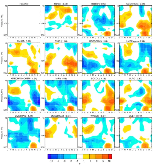
Figures 9–10 show trend errors with respect to the Rosenlof and Hassler data sets correspondingly. The ma-jority of the models underestimate the springtime depletion compared with the Hassler data set but not with the Rosenlof data set. Several models simulate too strong ozone depletion below 100 hPa in summer comparing with the three observa-tion data sets. In some models (LMDZrepro, WACCM) this may be a result of a delayed polar vortex break up (Eyring et al., 2006). MULTI and several individual models show bet-ter agreement with the Rosenlof data set (and also with the Hassler data set) than the two other observation data sets.

(9)

Rosenlof

100 10

Pressure, hPa

500

Randel

100 10

500

Hassler

100 10

500

CCSRNIES

100 10

500 CMAM

100 10

Pressure, hPa

500

E39C

100 10

500

GEOSCCM

100 10

500

LMDZrepro

100 10

500 MAECHAM4CHEM

100 10

Pressure, hPa

500

MRI

100 10

500

SOCOL

100 10

500

ULAQ

100 10

500 UMETRAC

100 10

Pressure, hPa

500

UMSLIMCAT

100 10

500

WACCM

100 10

500

MULTI

100 10

500

3.75 7.50 11.25 15.00 18.75 [mPa]

Fig. 5. Vertical ozone distribution climatology (1980–1984) in observational data sets (Rosenlof, Randel, Hassler), individual CCMVal models, and multi-model average (MULTI).

To investigate whether the choice of reference data set has a large impact on the model ranking we calculate Spearman’s rank correlation coefficient between model ranks in the same diagnostic but calculated with respect to different observa-tion data sets. There is a high correlaobserva-tion between the model ranks in ozone profile trends with respect to the Rosenlof and Randel data sets (r= 0.93) however the model ranks with re-spect to the Hassler data set are poorly correlated with those with respect to either the Rosenlof (r= 0.41) or the Randel (r= 0.56) data sets. Similar tests performed for the model ranks in the ozone profile climatology showed a high cor-relation between the ranks with respect to the Rosenlof and Hassler data sets (r= 0.93) but lower correlations between the model ranks with respect to the Randel data set and ei-ther the Rosenlof (r= 0.60) or the Hassler (r= 0.54) data sets. Model ranks in the total ozone climatology and trends were very similar with respect to both datasets (r>0.9).

4.3 Performance index and its uncertainty

Performance indices calculated using Eq. (4) are shown in Fig. 11 together with errors for the individual diagnostics. Comparing individual models shows that no one model per-forms better than the others in all diagnostics however some models have generally low errors while other have generally high errors. MULTI does not perform better than the individ-ual models in all diagnostics however its combined error is the lowest.

(10)

Fig. 6.Normalised errors with respect to the Rosenlof data set in vertical ozone distribution climatology shown in Fig. 5. Numbers next to data set names indicate domain-averaged errors normalised by the average error across the individual models according to Eq. (2).

To assess the robustness of our model ranking we perform several sensitivity tests. The sensitivity of the ranking to the choice of the reference data sets is assessed by calculating the performance indices using the individual reference data sets separately. Since for the Randel and Hassler data sets we do not have corresponding total ozone timeseries, these data sets are used in combination with the TOMS/SBUV data set. To study sensitivity of the results to sampling errors we use ad-ditional runs available for SOCOL, MRI, and WACCM. The calculations were repeated for two additional simulations for each of these models. Also we apply small modifications to the original diagnostics, which include restricting the domain to above 200 hPa, weighting the ozone profile errors accord-ing to the mass or geometric thickness of the correspondaccord-ing layer, or calculating the total ozone climatology diagnostic over the SH only. The performance indices calculated in these sensitivity tests are shown in Fig. 11 and provide an estimate of the ranking uncertainty. The changes in the per-formance indices in these experiments are up to 15% (about

0.1 in absolute units), suggesting that smaller differences in performance index between models may be insignificant. In terms of ranking, these changes resulted in models ranking changes by 0–2 positions. In all the tests MULTI gets the highest rank.

We also test the sensitivity of the ranking to the choice of model performance metric. Here, instead of applying Eqs. (1)–(4) we use an index similar to the one used in WE08: gj kl=1− 1

nW X

i

X

m

(wim

x_{imj l}−y_imkl

/σ_imkl), (6) wherenis a scaling factor, andgj klis the grade ofj-th model

inl-th diagnostic with respect tok-th reference data set. Neg-ative values ofg, wherever they are obtained, are set to zero. The maximum possible grade is 1. A zero grade means that the differences between the model and the observation in av-erage exceednσ. The model grade for an individual diag-nosticgj lis calculated as an average over model grades with

(11)

Rosenlof ( 0.43)

100 10

Pressure, hPa

500

Randel ( 0.62)

100 10

500

Hassler

100 10

500

CCSRNIES ( 0.84)

100 10

500 CMAM ( 0.63)

100 10

Pressure, hPa

500

E39C ( 1.08)

100 10

500

GEOSCCM ( 1.15)

100 10

500

LMDZrepro ( 0.79)

100 10

Pressure, hPa

500

MRI ( 1.52)

100 10

500

SOCOL ( 0.53)

100 10

500

ULAQ ( 0.86)

100 10

500 UMETRAC ( 0.58)

100 10

Pressure, hPa

500

UMSLIMCAT ( 0.88)

100 10

500

WACCM ( 0.80)

100 10

500

MULTI ( 0.56)

100 10

500

-20 -10 -5 -3 -1 1 3 5 10 20

σ

Fig. 7.The same as in Fig. 6 but with respect to the Hassler data set.

gjis calculated by averaging over the grades for the

individ-ual diagnostics.

The model grading calculated using Eq. (6) depends on the choice of the scaling factorn. If we choosen=3, as in WE08, then almost all the grades in the both climatol-ogy diagnostics are zero, the only exception being the total ozone climatology diagnostic in UMSLIMCAT. As a result, the combined model grades are determined by the trend di-agnostics only. Nevertheless, Spearman’s correlation coeffi-cient between the model ranks calculated using Eq. (6) and the original ranks is high (r= 0.86), although some individ-ual models change their ranks by 3–4 positions. Increasing nto 5 results in a small improvement of the correlation coef-ficient (r= 0.89) but further increases lead to converging of the grades in the trend diagnostics towards 1, thus decreas-ing the differences between the model grades in the trend diagnostics. As a result, the overall model grades are largely determined by the climatology diagnostics. MULTI typically gets the highest rank, except whennvaries between 4 and 6. In these cases, MULTI gets the second rank, and

UMSLIM-CAT gets the highest rank. This is because UMSLIMUMSLIM-CAT gets high grade in the total ozone climatology while the ma-jority of the models get zero grades in this diagnostic. De-spite these discrepancies the ranking obtained using Eq. (6) is in a reasonable agreement with the ranking obtained using Eqs. (1)–(4), with correlation coefficients exceeding 0.8.

4.4 Comparison with previous studies

(12)

Rosenlof

J F M A M JJ A S O N D J

100 10

Pressure, hPa

500

-6.9

Randel

100 10

500

-9.1

Hassler

100 10

500

-11.1

CCSRNIES

100 10

500

-5.3

CMAM

100 10

Pressure, hPa

500

-5.5

E39C

100 10

500

-4.3

GEOSCCM

100 10

500

-9.3

LMDZrepro

100 10

500

-9.0

MAECHAM4CHEM

100 10

Pressure, hPa

500

-14.3

MRI

100 10

500

-10.0

SOCOL

100 10

500

-4.6

ULAQ

100 10

500

-8.8

UMETRAC

100 10

Pressure, hPa

500

-10.5

UMSLIMCAT

100 10

500

-7.2

WACCM

100 10

500

-8.0

MULTI

100 10

500

-7.3

-6.0 -4.0 -2.0 -1.0 -0.5 0.5 1.0 2.0 4.0 6.0 [mPa per 20 years]

Fig. 8. 20-yr vertical ozone distribution trends (19808–1999) in observational data sets (Rosenlof, Randel, Hassler), individual CCMVal models, and multi-model average (MULTI). Red numbers indicate minimum trends.

intermediate performance index are small compared to the overall spread of the errors we conclude that our ranking is in a reasonable agreement with results by Eyring et al. (2006).

WE08 evaluated a subset of key processes important for stratospheric ozone, with the focus mainly on diagnostics to evaluate transport and dynamics in the CCMs. Spearman’s rank correlation coefficient between our model ranking and theirs is 0.59. WE08 also provide model grades based sep-arately on transport diagnostics or polar dynamic diagnos-tics. The agreement with our ranking gets worse if we con-sider either grades based on transport diagnostics (r= 0.44) or grades based on polar dynamic diagnostics (r= 0.54). In the case of polar dynamics diagnostics the most consider-able difference is that WACCM which has the highest per-formance index among the individual models in our anal-ysis gets low grade in the polar dynamics diagnostics be-cause of low grade in the zonal wind diagnostic (Eyring et al., 2006; WE08). The differences between our grades may be explained by, first, taking into account that some

impor-tant diagnostics (e.g. those related to polar chemistry) may be not considered in their study, and second, that those diag-nostics that were considered may need to be given different weights depending on their importance for polar ozone.

(13)

Rosenlof

100 10

Pressure, hPa

500

Randel ( 0.70)

100 10

500

Hassler ( 0.95)

100 10

500

CCSRNIES ( 0.91)

100 10

500 CMAM ( 0.62)

100 10

Pressure, hPa

500

E39C ( 1.08)

100 10

500

GEOSCCM ( 1.04)

100 10

500

LMDZrepro ( 0.94)

100 10

Pressure, hPa

500

MRI ( 1.03)

100 10

500

SOCOL ( 1.13)

100 10

500

ULAQ ( 0.87)

100 10

500 UMETRAC ( 1.11)

100 10

Pressure, hPa

500

UMSLIMCAT ( 0.74)

100 10

500

WACCM ( 0.64)

100 10

500

MULTI ( 0.49)

100 10

500

-10 -5 -3 -2 -1 1 2 3 5 10

σ

Fig. 9.Normalised errors with respect to the Rosenlof data set in vertical ozone distribution trends shown in Fig. 8. Numbers next to data set names indicate domain-averaged errors normalised by the average error across the individual models according to Eq (2).

simulations that require prescribed ozone fields. WE08 also noticed that weighting the model results according to their performance does not change significantly the multi-model average projection.

5 Conclusions

The goal of this study is to provide the climate mod-elling community with some recommendations regarding the choice of future ozone scenario for implementation in cli-mate simulations. We have validated the abilities of twelve CCMs to simulate the observed total ozone climatology and trends and also the Antarctic ozone profile climatology and trends and ranked the models according to their errors av-eraged across four chosen diagnostics. No one model per-forms better than the others in all four diagnostics; however combining errors in individual diagnostics into one metric of model performance allowed us to objectively rank the

mod-els. The highest rank is obtained by the multi-model en-semble average. Sensitivity tests performed to assess the robustness of the ranking showed that the individual mod-els may change their rank by several positions but that the multi-model ensemble average gets the highest rank in the majority of the experiments. Therefore we argue that the multi-model averaged projection, which is less sensitive to individual model biases, provides the best estimate of future ozone.

(14)

Rosenlof ( 0.76)

100 10

Pressure, hPa

500

Randel ( 0.84)

100 10

500

Hassler

100 10

500

CCSRNIES ( 1.16)

100 10

500 CMAM ( 0.99)

100 10

Pressure, hPa

500

E39C ( 1.27)

100 10

500

GEOSCCM ( 0.99)

100 10

500

LMDZrepro ( 0.85)

100 10

Pressure, hPa

500

MRI ( 0.78)

100 10

500

SOCOL ( 1.20)

100 10

500

ULAQ ( 0.94)

100 10

500 UMETRAC ( 0.78)

100 10

Pressure, hPa

500

UMSLIMCAT ( 0.89)

100 10

500

WACCM ( 0.70)

100 10

500

MULTI ( 0.71)

100 10

500

-10 -5 -3 -2 -1 1 2 3 5 10

σ

Fig. 10.The same as in Fig. 9 but with respect to the Hassler data set.

0.0 0.5 1.0 1.5 2.0 2.5 3.0

Error

CCSRNIES CMAM E39C

GEOSCCM LMDZrepro

MAECHAM4CHEM MRI

SOCOL ULAQ UMETRAC

UMSLIMCAT WACCM MULTI - Total ozone climatology error - Ozone profile climatology error - Total ozone trend error

- Ozone profile trend error - Performance index

Fig. 11.Model performance index and errors in individual diagnos-tics. Performance indices from sensitivity tests are marked by grey bars.

study, were not considered by WE08 or because those di-agnostics that were considered may need to be given differ-ent weights depending on their importance for polar ozone. This comparison shows that the selection of diagnostics for process-oriented CCM validation remains a challenging task and depends on the region of interest.

(15)

the need for the compilation of a unified reliable vertically resolved ozone reference data set.

Our assessment has at least two practical applications. First, modellers can make a choice of future ozone scenario based on the quantitative evaluation. Second, ozone simu-lations by future model generations can be validated in the same way as done here and model improvements can be quantitatively assessed.

Acknowledgements. This work is supported by NERC Project NE/E006787/1. We acknowledge the modeling groups for making their simulations available for this analysis, the Chemistry-Climate Model Validation Activity (CCMVal) for WCRP’s (World Climate Research Programme) SPARC (Stratospheric Processes and their Role in Climate) project for organizing and coordinating the model data analysis activity, and the British Atmospheric Data Center (BADC) for collecting and archiving the CCMVal model output. We thank TOMS/SBUV team and W. Randel for making their data sets publicly available and also V. Eyring, M. Dameris, J. Scinocca, T. Reichler, and an anonymous reviewer for useful comments.

Edited by: L. Carpenter

References

Akiyoshi, H., Sugita, T., Kanzawa, H., and Kawamoto, N.: Ozone perturbations in the Arctic summer lower stratosphere as a re-flection of NOxchemistry and planetary scale wave activity, J. Geophys. Res., 109, D03304, doi:10.1029/2003JD003632, 2004. Austin, J., Wilson, R. J., Li, F., and Vomel, H.: Evolution of wa-ter vapor concentrations and stratospheric age of air in coupled chemistry-climate model simulations, J. Atmos. Sci., 64, 905– 921, 2006.

Bracegirdle, T. J., Connolley, W. M., and Turner J.: Antarctic cli-mate change over the twenty first century, J. Geophys. Res., 113, D03103, doi:10.1029/2007JD008933, 2008.

Br¨uhl, C., Crutzen, P. J., and Grooß, J. U.: High-latitude, sum-mertime NOx activation and seasonal ozone decline in the lower stratosphere: Model calculations based on observations by HALOE on UARS, J. Geophys. Res., 103, 3587–3597, 1998. Cai, W., Shi, G., and Li, Y.: Multidecadal fluctuations of

win-ter rainfall over southwest Weswin-tern Australia simulated in the CSIRO Mark 3 coupled model. Geophys. Res. Lett., 32, L12701, doi:10.1029/2005GL022712, 2005.

Connolley, W. M. and Bracegirdle, T. J.: An Antarctic assessment of IPCC AR4 climate models, Geophys. Res. Lett., 34, L22505, doi:10.1029/2007GL031648, 2007.

Dall’Amico, M., Gray, L. J., Rosenlof, K. H., Scaife, A. A., Shine, K. P., and Stott, P. A.: Stratospheric temperature trends: impact of ozone variability and the QBO, Clim. Dynam., 34(2–3), 381– 398, doi:10.1007/s00382-009-0604-x, 2010.

Dameris, M., Grewe, V., Ponater, M., Deckert, R., Eyring, V., Mager, F., Matthes, S., Schnadt, C., Stenke, A., Steil, B., Br¨uhl, C., and Giorgetta, M.: Long-term changes and variability in a transient simulation with a chemistry-climate model employing realistic forcings, Atmos. Chem. Phys., 5, 2121–2145, 2005, http://www.atmos-chem-phys.net/5/2121/2005/.

Egorova, T., Rozanov, E., Zubov, V., Manzini, E., Schmutz, W., and Peter, T.: Chemistry-climate model SOCOL: a validation of

the present-day climatology, Atmos. Chem. Phys., 5, 1557–1576, 2005, http://www.atmos-chem-phys.net/5/1557/2005/.

Eyring, V., Butchart, N., Waugh, D. W., et al.: Assessment of tem-perature, trace species, and ozone in chemistry-climate model simulations of the recent past, J. Geophys. Res., 111, D22308, doi:10.1029/2006JD007327, 2006.

Eyring, V., Waugh, D. W., Bodeker, G. E., et al.: Multimodel pro-jections of stratospheric ozone in the 21st century, J. Geophys. Res., 112, D16303, doi:10.1029/2006JD008332, 2007.

Fomichev, V. I., Jonsson, A. I., de Grandpr’e, J., et al.: Response of the middle atmosphere to CO2 doubling: Results from the Cana-dian Middle Atmosphere Model, J. Climate, 20, 1121–1144, 2007.

Fyfe, J. C., Boer, G., and Flato, G.: The Arctic and Antarctic Oscil-lations and their projected changes under global warming, Geo-phys. Res. Lett., 26, 1601–1604, 1999.

Garcia, R. R., Marsh, D., Kinnison, D., Boville, B., and Sassi, F.: Simulations of secular trends in the middle at-mosphere, 1950–2003, J. Geophys. Res., 112, D09301, doi:10.1029/2006JD007485, 2007.

Gillett, N. P. and Thompson, D. W. J.: Simulation of recent South-ern Hemisphere climate change, Science, 302, 273–275, 2003. Gleckler, P. J., Taylor, K. E., and Doutriaux, C.: Performance

metrics for climate models, J. Geophys. Res., 113, D06104, doi:10.1029/2007JD008972, 2008.

Hassler, B., Bodeker, G. E., and Dameris, M.: Technical Note: A new global database of trace gases and aerosols from multiple sources of high vertical resolution measurements, Atmos. Chem. Phys., 8, 5403–5421, 2008

Hassler, B., Bodeker, G. E., Cionni, I., and Dameris, M.: A verti-cally resolved, monthly mean, ozone database from 1979 to 2100 for constraining global climate model simulations, International Journal of Remote Sensing, Int. J. Remote Sens., 30(15), 4009-4018, doi:10.1080/01431160902821874, 2009.

Hu, Y. and Tung, K. K.: Interannual and decadal variations of plan-etary wave activity, stratospheric cooling, and Northern Hemi-sphere annular mode, J. Climate, 15,1659–1673, 2002. Hu, Y., Tung, K. K., and Liu, J.: A Closer Comparison of Early and

Late-Winter Atmospheric Trends in the Northern Hemisphere, J. Climate, 18, 3204–3216, 2005.

Jourdain, L., Bekki, S., Lott, F., and Lef`evre, F.: The coupled chemistry-climate model LMDz-REPROBUS: description and evaluation of a transient simulation of the period 1980–1999, Ann. Geophys., 26, 1391–1413, 2008,

http://www.ann-geophys.net/26/1391/2008/.

Karpetchko, A. and Nikulin, G.: Influence of early winter upward wave activity flux on midwinter circulation in the stratosphere and troposphere, J. Climate, 17, 4443–4452, 2004.

Marshall, G. J., Orr, A., van Lipzig, N. P. M., and King, J. C.: The Impact of a Changing Southern Hemisphere Annular Mode on Antarctic Peninsula Summer Temperatures, J. Climate, 19,

5388–5404, 2006.

Miller, R. L., Schmidt, G. A., and Shindell, D. T.: Forced annu-lar variations in the 20th century Intergovernmental Panel on Climate Change Fourth Assessment Report models, J. Geophys. Res., 111, D18101, doi:10.1029/2005JD006323, 2006.

(16)

Strato-spheric Ozone-Temperature Coupling Between 1950 and 2005, J. Geophys. Res., 113, D12103, doi:10.1029/2007JD009511, 2008.

Pitari, G., Mancini, E., Rizi, V., and Shindell, D.: Feedback of future climate and sulfur emission changes an stratospheric aerosols and ozone, J. Atmos. Sci., 59, 414–440, 2002.

Perlwitz, J., Pawson, S., Fogt, R. L., Nielsen, J. E., and Neff, W. D.: Impact of stratospheric ozone hole recovery on Antarctic climate, Geophys. Res. Lett., 35, L08714, doi:10.1029/2008GL033317, 2008.

Randel, W. J. and Wu F.: Cooling of the Arctic and Antarctic polar stratospheres due to ozone depletion, J. Climate, 12, 1467–1479, 1999.

Randel, W. J. and Wu F.: A stratospheric ozone profile data set for 1979–2005: Variability, trends, and comparisons with column ozone data, J. Geophys. Res., 112, D06313, doi:10.1029/2006JD007339, 2007.

Reichler, T. and Kim, J.: How well do coupled models simulate today’s climate?, B. Am. Meteorol. Soc., 89, 303–311, 2008. Schraner, M., Rozanov, E., Schnadt Poberaj, C., Kenzelmann, P.,

Fischer, A. M., Zubov, V., Luo, B. P., Hoyle, C. R., Egorova, T., Fueglistaler, S., Bronnimann, S., Schmutz, W., and Peter, T.: Technical Note: Chemistry-climate model SOCOL: version 2.0 with improved transport and chemistry/microphysics schemes, Atmos. Chem. Phys., 8, 5957–5974, 2008,

http://www.atmos-chem-phys.net/8/5957/2008/.

Shibata, K. and Deushi, M.: Partitioning between resolved wave forcing and unresolved gravity wave forcing to the quasi-biennial oscillation as revealed with a coupled chemistry-climate model, Geophys. Res. Lett., L12820, doi:10.1029/2005GL022885, 2005.

Son, S.-W., Polvani, L. M., Waugh, D. W., Akiyoshi, H., Garcia, R., Kinnison, D., Pawson, S., Rozanov, E., Shepherd, T. G., and Shi-bata, K.: The Impact of Stratospheric Ozone Recovery on the Southern Hemisphere Westerly Jet, Science, 320, 1486–1489, 2008.

Son, S.-W., Tandon, N. F., Polvani, L. M., and Waugh, D. W.: Ozone hole and Southern Hemisphere climate change, Geophys. Res. Lett., 36, L15705, doi:10.1029/2009GL038671, 2009. Steil, B., Br¨uhl, C., Manzini, E., Crutzen, P. J., Lelieveld, J., Rasch,

P. J., Roeckner, E., and Kr¨uger, K.: A new interactive chem-istry climate model, 1: Present day climatology and interan-nual variability of the middle atmosphere using the model and 9 years of HALOE/UARS data, J. Geophys. Res., 108, 4290, doi:10.1029/2002JD002971, 2003.

Stolarski, R. S. and Frith, S.: Search for evidence of trend slowdown in the long-term TOMS/SBUV total ozone data record: The im-portance of instrument drift uncertainty, Atmos. Chem. Phys., 6, 4057–4065, 2006,

Thompson, D. W. J. and Solomon, S., Interpretation of recent Southern Hemisphere climate change, Science, 296, 895–899, 2002.

Tian, W. and Chipperfield, M. P.: A new coupled chemistry-climate model for the stratosphere: The importance of coupling for future O3-climate predictions, Q. J. Roy. Meteor. Soc., 131, 281–304, 2005.

Waugh, D. W. and Eyring, V.: Quantitative performance met-rics for stratospheric-resolving chemistry-climate models, At-mos. Chem. Phys., 8, 5699–5713, 2008,

World Meteorological Organization (WMO)/United Nations Envi-ronment Programme (UNEP): Scientific Assessment of Ozone Depletion: 2006, World Meteorological Organization, Global Ozone Research and Monitoring Project, Report No. 50, Geneva, Switzerland, 2007.